Forecasting International Tourism Demand Using a Non-Linear Autoregressive Neural Network and Genetic Programming

Abstract

This study explores the forecasting ability of two powerful non-linear computational methods: artificial neural networks and genetic programming. We use as a case of study the monthly international tourism demand in Spain, approximated by the number of tourist arrivals and of overnight stays. The forecasting results reveal that non-linear methods achieve slightly better predictions than those obtained by a traditional forecasting technique, the seasonal autoregressive integrated moving average (SARIMA) approach. This slight forecasting improvement was close to being statistically significant. Forecasters must judge whether the high cost of implementing these computational methods is worthwhile.

1. Introduction

Tourism demand forecasting is a relevant and stimulating topic for different agents involved in the tourism sector, such as practitioners and policy makers [1]. Access to good forecasts would help these agents to anticipate future demand for tourism and conveniently adapt their supply capacities. Tourism-related resources could be allocated more efficiently, and the sector would be able to produce more profit. For this reason, it is of crucial importance for researchers and operational managers to select a forecasting method that provides the highest predictive accuracy. We can find in the specialized literature different methods to model and predict the dynamic evolution of the demand for tourism. Basically, these methods are usually split into two categories: regression-based models and time series models [2].

The regression-based models are based on economic theory, and they attempt to forecast tourism demand using socio-economic variables such as population, income, price level, substitute prices, and marketing expenditures on promotional activities [3]. Some authors have also included in the models other relevant explanatory variables to gather the influence of meteorological and cultural effects on tourism demand [4]. The aim of these regression-based models is not only to forecast, but also to investigate which are the main determinants of tourism demand. This additional issue is extremely relevant for the tourism industry, since it is possible to quantify the impact of these determinants on demand, and generate simulations from which policy recommendations can be derived. Nevertheless, the regression-based models are not exempt from problems that limit their usefulness in obtaining good forecasts. First, it is difficult to discover and establish the basic principles to build an optimal model. Second, there are usually measurement errors in the explanatory variables that can produce negative effects on the predictive accuracy of the model. Finally, we often do not have the current values of the explanatory variables, and we need to make use of their predicted values.

The other modeling category, time series models, only uses historical values of the variable to be predicted. This procedure is less time consuming and less costly than regression-based models, the informational requirement is minimal, and they are simpler and easy to use [5]. These advantages make this approach very attractive, but it has frequently been criticized because it is not based on the principles of economic theory. However, very often, the only objective of economic agents is to reach accurate forecasts, regardless of whether they are derived from a model based on an economic background. Economists should be more pragmatic. They should pay less attention to models that attempt to understand the complexity of the economy, and concentrate more on models that predict the future acceptably. According to this pragmatic thought, previous research on tourism demand forecasting has demonstrated that time series models very often provide more accurate out-of-sample forecasts than regression-based models [6,7,8,9,10]. In the competition carried out in [11], the superior forecasting ability of the time series models was verified.

The adoption of time series methods has become very popular in tourism demand forecasting; most notably, the autoregressive integrated moving average (ARIMA) models [12,13]. The seasonal extension of the ARIMA model, the seasonal autoregressive integrated moving average (SARIMA) model, has also been widely employed to predict tourism demand [2,14]. The main reason for its popularity is that monthly or quarterly forecasts tend to be more useful in strategic marketing or operational planning, and the SARIMA method can capture quite well the strong seasonal patterns observed in tourism data. However, the ARIMA and SARIMA models, as well as the great majority of the time series models used in tourism demand forecasting, are commonly based on a parametric and linear perspective. Specifically, the researchers usually specify a priori a specific linear functional form of the models, with a set of unknown parameters that are estimated using some optimization procedure (e.g., ordinary least squares).

Recent empirical results support that tourism time series contain important and predictable non-linear patterns [15,16]. Consequently, the assumption of linearity seems to be too rigid, and it is possibly constraining our predictive ability. Some authors have adopted a parametric approach but assuming a nonlinear structure of the model [17]. Despite this, it seems that the insertion of specific nonlinearities into the parametric models does not imply a clear forecasting gain. It is possible that the failure of these non-linear parametric models may be due to the fact that the non-linear structure is forced by the researcher rather than observed in the data. In other words, the researcher chooses one particular nonlinear specification that may not be general enough to capture all nonlinearities existing in the data [18]. It seems, therefore, to be recommendable to use a more flexible modeling approach.

Today, the use of forecasting methods based on a non-parametric approach has emerged thanks to remarkable advances in computer hardware and software. These methods show the great advantage of being very flexible regarding the functional form of the model. To be more precise, the forecaster does not determine a priori any discretional assumptions on the functional form of the model. Indeed, it is the method itself that selects the optimal inputs and determines the functional form of the model. The approach is based on the fact that it lets the data speak for itself (i.e., it is a data-driven approach). The main advantage of these methods is that they allow us to exploit any non-linearity existing in the data, which should increase our predictive capacity. Applied econometricians have rapidly included all these methods into their toolbox to analyze and predict different economic and financial time series, including the prediction of tourism demand. In this regard, artificial neural networks (ANNs) have been by far the most popular non-parametric method used in modeling and forecasting tourism demand [2]. However, the method is very often criticized for the requirement of a large data set and the complex and tedious process of designing an optimal architecture. In our study, we explore the predictive accuracy of a non-linear autoregressive neural (NAR) network to predict tourism demand data. The popular parametric SARIMA approach is used as a benchmark against which to compare the forecasting accuracy of the proposed non-parametric methods. We also introduce a novel non-parametric forecasting method called genetic programming (GP) [19]. This method comprises a wide range of different procedures founded on the Darwinian concepts of natural selection and survival of the fittest individual. GP has theoretically demonstrated a good ability to predict variables characterized by a complex dynamic [20,21,22], included chaotic structures, but its use in tourism demand forecasting has been rather scarce.

The problem of tourism demand forecasting is not new, but there is certain controversy on whether the non-parametric methods are capable of improving the forecasting accuracy of the parametric ones (that is to say, the capacity of the nonparametric methods, and more specifically of the ANNs, to predict tourism demand is in question). While some studies find evidence in favor of the superior forecasting performance of ANNs [23,24,25,26,27], others claim that simple ARIMA-based models provide more accurate tourism demand forecasts [28,29]. In this regard, [30] concludes that SARIMA models could show some advantage in short-term predictions, as long as there is not a structural change in the time series.

Our study sheds some light on this debate. In particular, our findings support the belief that NAR networks are capable of providing more accurate forecasts than those reached by the SARIMA model. In our opinion, this study also makes some additional contributions to the extant literature:

-

First, the use of artificial neural networks and SARIMA models are common in tourism forecasting; however, the use of GP is still very scarce. There are not many studies that have analyzed and compared the predictive performance of GP in tourism time series.

-

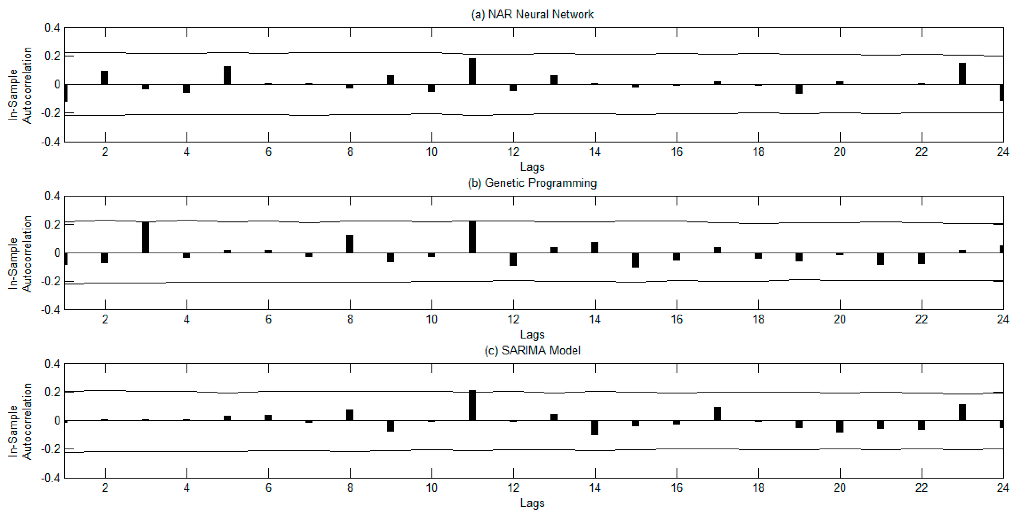
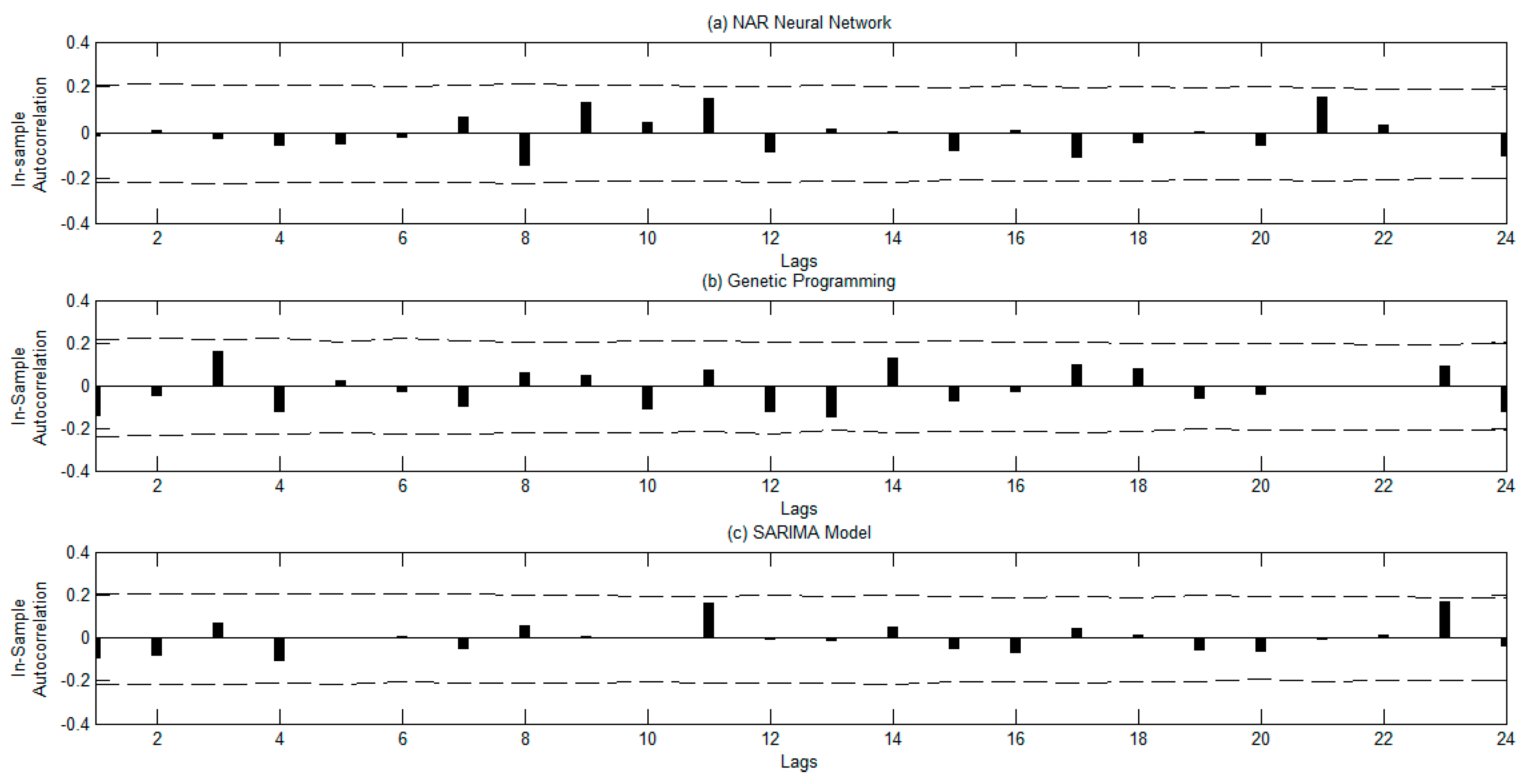
Second, the robustness of the forecasting methods is checked by using the autocorrelation function of the residuals and the surrogate method. The diagnosis checking is a necessary step frequently omitted in tourism forecasting.

-

Third, we check if there are statistical differences between the forecasts of the two competing methods by using a novel approach based on the bootstrap method and on the estimation of empirical distributions of probability through the kernel method.

-

Last but not least, the forecasting study presented here is based on a data set related to the international demand for tourism to Spain. International tourism demand in Spain has grown rapidly in recent decades, becoming one of the most important sectors for the Spanish economy. Even more important, the economic contribution of international tourism is playing a proactive role to fuel the economy of Spain, and mitigate the negative effects of the deep economic crisis that hit the country in recent years. For all these reasons, international tourism demand forecasting has become a specific focal point of interest for Spanish policymakers.

The organization of this study is as follows. After this introductory section, in Section 2, we briefly explain the non-linear forecasting methods used in our forecasting study. In Section 3, we show our main forecasting results. Additionally, in this section, we also describe the data and explain certain important technical aspects. Finally, we conclude and discuss the main results in Section 4.

2. Forecasting Methods

2.1. Artificial Neural Networks

Artificial neural networks are mathematical models that are inspired by how biological neurons work and are organized. The purpose of this section is to present a brief overview of this computer-based modeling procedure. For a more detailed technical explanation about artificial neural networks, the reader is referred to the books by [31,32]; and for empirical applications, recommended reading includes [33,34]. In all these references, we can see that there are many different types of neural network models that can be used for forecasting purposes, such as radial basis or recurrent networks. The neural network that was used in our specific forecasting study is a feed-forward multi-layer network with a learning algorithm based on the back-propagation algorithm. This network is by far the most popular and successful to predict economic and financial series [35], as well as tourism data [36,37]. The main reason for its popularity is that many theoretical studies have shown that this network can reflect any non-linear dynamic with a certain level of accuracy [38,39]. In particular, we use in our study a non-linear autoregressive neural (NAR) network. This kind of network is assumed to be a general nonlinear autoregressive model, and is formally represented as follows

$$x_t=\mathsf{\Phi }\left({\beta }_0+{\displaystyle \sum }_{h=1}^H{\beta }_h·\left({\mathsf{\Psi }}_h\left({\alpha }_{h0}+{\displaystyle \sum }_{p=1}^P{\vartheta }_{hp}·x_{t-p}\right)\right)\right)+{\epsilon }_t$$

(1)

where $\left\{x_t\right\}$ is the time series to be predicted, ${\mathsf{\Psi }}_h(·)$ and $\mathsf{\Phi }(·)$ are the transfer functions, P is the number of input nodes (i.e., lags of the variable), and H is the number of hidden nodes. The parameters of the model ${\beta }_0$, ${\beta }_h$, ${\alpha }_{h0}$ and ${\alpha }_{hp}$ are the weights of the network. The initial values of these weights are randomly set within a determined range. The weights are modified through an iterative learning process based on the back-propagation algorithm [40] to minimize the sum of the squared errors (SSE). The iterative process finishes when a predetermined number of iterations is reached, or when the SSE falls below a desirable value. As usual, ${\epsilon }_t$ is the disturbance term, which is assumed to be an independent and identically distributed (i.i.d) random variable.

The predictive ability of the NAR neural network designed in our study basically relies on the complexity of the data, but also on the correct selection of a suitable specification of the network. The network design is done through a complex process in which a large number of technical parameters must be determined to ensure a good forecasting performance of network. Among these technical parameters, it is critical to adequately select (i) the transfer functions, and to determine appropriately (ii) the number of lags (P) and (iii) the number of hidden nodes (H). Regarding the transfer functions, it is usually recommended in the literature to use a linear structure for $\mathsf{\Phi }(·)$ and a sigmoid function for ${\mathsf{\Psi }}_h(·)$ [41]. Another important point is how to specify the upper bounds of the summations in Equation (1). That is, it is necessary to establish an optimal specification of the number of input nodes (P) and hidden nodes (H) of the network. Too few nodes may cause the network to not be capable of reflecting satisfactorily the dynamic shown by the data. Conversely, too many nodes may result in a poor forecasting ability when the network predicts observations that were not considered in the model-selection process (i.e., overfitting problems). In the specialized literature, there are no clear instructions on how to optimally select P and H. Nonetheless, a common recommendation is to choose these values through experimentation [18]. In particular, in our study, we adopt the fixed approach explained in [42]. Briefly, the fixed approach is based on designing numerous networks assuming different values of H and P. In our study, we consider values of P from 1 to 20, and values of H from 1 to 5. Therefore, in total, more than one hundred networks were designed. The forecasting power of each one of these networks is evaluated in a specific set of data, and the network that provides the most accurate forecasts is finally chosen to make out-of-sample predictions.

2.2. Genetic Programming

The term genetic algorithms includes a broad set of computing procedures. All these procedures have in common the use of biological concepts and are inspired in the theory of the evolution of species. Genetic programming (GP), one specific procedure based on genetic algorithms, artificially reproduces in a computer an evolutionary process with the aim of finding a mathematical equation that optimally approximates the dynamic of the data over time. GP has shown success in modeling the data-generating process of one-dimensional time series [20,21,22], as well as spatio-temporal time series [43]. GP offers some important advantages in comparison with other non-parametric computational forecasting methods (e.g., artificial neural networks). First, GP does not require the tedious process of constructing the network. Second, and more important, GP offers a mathematical equation that is supposed to optimally approximate the dynamic of a time series.

The GP used in our study was programmed in FORTRAN, according to the technical instructions given in [22]. In particular, following the steps explained in [20,21,22], the GP begins generating a random initial population of N mathematical equations:

$$Equatio{n}_j: {\widehat{x}}_{t,j}=\left(\left(A Op B\right) Op \left(C Op D\right)\right) \forall j, 1\le j\le N$$

(2)

where A, B, C, and D are the arguments (i.e., real numbers or lagged values of the time series), and ‘Op’ stands for one of the four arithmetic operators (i.e., addition, subtraction, multiplication and division). The subscript j denotes each one of the N equations belonging to the initial population.

In a second step, the GP assesses the strength of each equation j of the initial population according to a specific criterion (i.e., how well the equation fits the data). In our case, we use the sum of the squared errors as the criterion to assess the goodness of fit of each equation j

$$SS{E}_j={\displaystyle \sum }_{t=1}^T{\left(x_t-{\widehat{x}}_{t,j}\right)}^2 \forall j=1,\dots ,N$$

(3)

where SSE is the sum of the squared errors (SSE) presented by the equation j-th ($\forall j, 1\le j\le N$), $x_t$ represents the time series evolution, ${\widehat{x}}_{t,j}$ is the predicted value of the equation j-th, and T is the total number of observations aimed to evolve the GP. The lower the SSE, the better the fit of the equation. Hence, those equations whose SSE is very high are removed, while those equations with a low SSE are more likely to survive and be part of the next generation of equations.

In the following step, the GP randomly selects some of the survival equations. The selected equations are used to generate a new population of N equations by using the genetic operators of cloning, crossover, and mutation. With cloning, the “fittest” equations are directly added without any modification to the new population of equations. With crossover, pairs of equations exchange part of their arguments (i.e., real numbers and lagged values) and their mathematical operators to originate new equations. Finally, the genetic operator mutation implies that any mathematical operator or argument can be randomly replaced in a reduced number of equations.

The described processes of evaluation, selection and mutation are iteratively repeated. After several repetitions pre-established by the forecaster, the evolutionary process generated by the GP finishes and provides a model that is the strongest mathematical equation of the last population. The setup of the GP used in our study is exactly the same as the one explained in [22]. The maximum number of arguments and mathematical operators in each equation was 26. Each generation had a maximum population of 260 equations and, in each case, we specify a maximum of 10,000 generations. The crossover and mutation rates are been 0.2 and 0.1, respectively. The adequacy of this setup is guaranteed by previous work [44]. Moreover, we conducted a sensitivity analysis in which the soundness of the technical setup was corroborated.

3. Results

3.1. Data and Assesment of Forecasting Performance

International demand for tourism is commonly understood as the combination of goods and services that non-residents want and can consume during their trips in the country of destination, considering as given the prices, income and other socio-economic variables.

There are different measures that have traditionally been used to approximate international tourism demand. Among them, the tourist expenditure and the number of tourist arrivals are the most common approximations to international tourism demand in empirical studies [3]. The use of one or the other approximation will depend basically on the objectives that have the different users of the tourism demand forecasts. As [2] indicates, tourism managers are more interested in forecasting the number of tourism arrivals, as this variable has a direct impact on supply capacity. On the other hand, tourist expenditure is a matter of more interest for policymakers such as governments or central banks. It is for this reason that a complete forecasting study of tourism demand should offer predictions of both demand measures. However, it is very difficult to have a reliable variable that adequately approximates the volume of expenditure generated by visitors from abroad [1]. Given this problem, many authors recommend substituting tourist expenditure by the number of tourist overnight stays [45]. Accordingly, we use as proxies for international tourism demand to Spain the number of tourist arrivals and of overnight stays spent by non-residents. The data of both variables came from the Hotel Occupancy Survey (HO) performed by the Spanish Statistical Institute (INE). The sample period goes from January 1999 to December 2012, having a total of 168 monthly observations to conduct our forecasting research. There are basically two reasons that justify the use of monthly data instead of annual data in our forecasting study. The first is that annual data cannot satisfactorily meet the forecasting requirements of the decision-makers in tourism. As stated by [2], it is much more interesting to predict monthly tourism demand data since these predictions are more useful to improve short-term business planning or resource management. The second reason is that it is possible to get more accurate and consistent predictions with monthly data since we have a larger amount of observations.

The variable to be predicted is the seasonal and non-seasonal difference of the tourism demand

$$x_t={\nabla }^1{\nabla }^{12}\log \left({\mathrm{Y}}_t\right)=\left(\log \left(Y_t\right)-\log ({\mathrm{Y}}_{t-12})\right)-\left(\log \left({\mathrm{Y}}_{t-1}\right)-\log \left({\mathrm{Y}}_{t-13}\right)\right)$$

(4)

where $Y_t$ is the measure of international tourist demand to Spain (i.e., the number of international tourism or overnight stays); log is the logarithmic transformation, and the symbols ${\nabla }^1$ and ${\nabla }^{12}$ stand for the first-order and twelfth-order operator, respectively. This data transformation is very usual in time series forecasting and, specifically, in tourism demand forecasting. On the one hand, the logarithm transformation simplifies and improves the modeling procedure since it reduces the variability and asymmetry existing in the data. On the other hand, taking differences makes the time series stationary, which is required to apply the forecasting methods considered in our forecasting research. As noted by [46,47], the data transformation defined in Equation (4) can be useful to increase the accuracy of the methods when predicting tourism time series. The transformed data $x_t$ are used to build the different forecasting methods employed in this study. The predictions obtained by the different methods are rescaled back in order to calculate the forecasting accuracy based on the original scale of the data (i.e., based on the scale of the original variable ${\mathrm{Y}}_t$).

Figure 1a shows the dynamic of the number of international overnights, while Figure 1b reflects the evolution of international tourist arrivals during the sample period. The most salient characteristic of these time plots is that the series have a slight upward trend and show a strong seasonal pattern. Figure 1c,d depicts the dynamic of the transformed series. In these series, we can observe how the trend and the seasonal components of the series have been completely removed. The use of the Ng-Perron unit root test reveals that our original series ${\mathrm{Y}}_t$, shown in Figure 1a,b, are non-stationaries at frequency zero. Additionally, the Hylleberg-Engle-Granger-Yoo (HEGY) test also detects the existence of seasonal unit roots. On the other hand, these tests provide evidence that the transformed series $x_t$ showed in Figure 1c,d are stationaries both at seasonal and non-seasonal frequencies. Figure 1 also informs us about how the whole sample period was split into three different sub-periods. This sample partition has been strongly recommended in computer science [31], economics and finance [44], and tourism forecasting [29,36] to restrict memorization of the network (i.e., overfitting) and, therefore, to conduct a complete, valuable and fair forecasting study. The first one is called the training/evolutionary period. It comprises the period from January 1999 to December 2009, containing the first 132 observations of the sample. The data contained in this subsample are employed to construct different NAR networks, and to get different equations through the evolutionary process recreated by the GP. The second subsample, the selection period, covers the period from January 2010 to December 2011, comprising a total of 24 observations. This sub-sample is used to choose the NAR network and the evolutionary equation that better fit the data. The addition of the training/evolutionary period and the selection period is called the in-sample data set. The last subsample is the out-of-sample and covers the twelve months of 2012. These untouched data have not been used in the modeling process. Therefore, the predictive accuracy measured in the out-of-sample must be the only valid to evaluate and compare the performance of the different forecasting methods.

An important question that remains at this point is to define an appropriate accuracy measure that assesses and compares the different predictive methods. Among the possible accuracy measures available in the literature, the most common and highly recommended is the mean absolute percentage error (MAPE) [48]. Moreover, as [3,7] point out, this measure is the most frequent and suitable in tourism demand forecasting. The reason for its widespread use lies in its numerous advantages. First, it is less sensitive to outliers; second, it is easy to interpret; third, it does not depend on the scale of the variable to be predicted and, finally, it allows us to easily compare the forecasting performance of different competing models [48]. The MAPE is specifically defined by the expression:

$$\mathrm{MAPE}=\frac{100}{T}·{\displaystyle \sum }_{t=1}^T\left|\frac{Y_t-{\widehat{Y}}_t}{Y_t}\right|$$

(5)

where $Y_t$ is the actual value of the international tourism demand to Spain, ${\widehat{Y}}_t$ is the predicted value, and T is the sample size of the period in which the forecasting performance is assessed. A word of caution is needed at this point. The predictions given by the different methods (${\widehat{x}}_t$) are rescaled back following the reverse of the data transformation, and the forecasting accuracy based on the MAPE is determined on the basis of the original scale of the tourism demand data ($Y_t$).

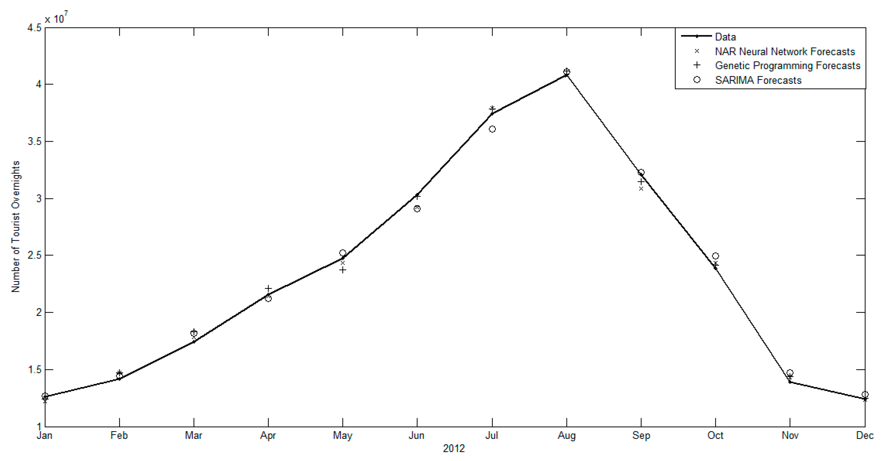
3.2. Forecasting Results

As mentioned earlier, we construct different NAR networks and evolutionary equations using the data belonging to the training/evolutionary period. Later on, we select those models that perform better in the selection period. One of the most important choices in non-linear modeling and forecasting time series is to determine the optimal number of lags for the model [41]. Figure 2 and Figure 3 show the sensitivity of the non-linear methods when different delays (p) are considered to predict international overnight stays and international tourist arrivals, respectively. As can be observed, the forecasting performance of the different non-linear methods shows a certain stability in the selection period, regardless of the number of delays that are considered. Nevertheless, and as is recommended in the specialized literature, we selected the number of lags that provided the lowest MAPE in the selection period. That is, for the prediction of international overnight stays, the optimum was achieved at lag 14 for the NAR network, and 13 for the genetic program. In the case of international tourist arrivals, the minimum MAPEs were at lags 17 for the NAR network, and 13 for the GP.

Unlike NAR networks and other non-linear forecasting methods, genetic programming has the great advantage of explicitly providing a mathematical equation that represents the dynamic of the time series to be predicted. In our study, these equations were, for the case of the prediction of the international overnights stays in Spain,

$${\widehat{x}}_t=-\frac{x_{t-1}·A\left(t\right)}{\left[2.09+8.64·x_{t-12}\right]·A\left(t\right)+x_{t-12}·x_{t-4}·\left[x_{t-4}-x_{t-7}\right]}$$

(6)

where $A\left(t\right)=x_{t-2}·9.68·x_{t-13}·\left[x_{t-4}-x_{t-7}\right]+x_{t-11}·x_{t-13}$.

And for the prediction of the international number of arrivals to Spain,

$${\widehat{x}}_t=-\frac{(x_{t-11}{x}_{t-12}-2.56·x_{t-1})·B\left(t\right)-2.56·x_{t-13}·x_{t-4}·x_{t-5}}{\left[4.97+x_{t-12}\right]·B\left(t\right)}$$

(7)

where $B\left(t\right)=5.97+x_{t-10}·x_{t-4}·x_{t-5}+x_{t-8}$. The optimal equations that survived the evolutionary process generated by the GP are similar for both time series. These equations reflect a clear non-linear dynamic, and show the importance of the lags around 12 to explain the dynamic of the series (specifically, at lags 11, 12, and 13). The importance of these lags is due to the strong non-linear seasonal pattern existing in the series, and the GP is capable of capturing it.

Most forecasting studies have basically chosen their forecasting models according to the accuracy of the predictions obtained by such models in the selection period. Even though this is an important criterion to select the best model, it is not the only one that must be taken into consideration. An additional criterion is that the errors of the selected models must not exhibit autocorrelation problems. In the case that the residuals were significantly correlated, the predictions would be sub-optimal, and it should be possible to improve the prediction [49]. However, and as [17] mentions, the problem is that tourism forecasters have frequently omitted the analysis of the residuals, which is essential in a complete forecasting study. In our case, Figure 4 and Figure 5 show autocorrelation function of the residuals of the models finally selected in the in-sample period. Their respective empirical intervals are also depicted. Following the indications given in [50], the empirical intervals are constructed by means of the surrogate method, assuming a level of confidence of 99 percent. Looking at these figures, we can observe that the residuals do not show any strong systematic pattern since none of the sample autocorrelation coefficients is significantly different from zero at 5 percent level (the no-autocorrelation of the residuals was also verified by the Ljung-Box test). Hence, the nonexistence of problems of autocorrelation suggests that both the NAR networks and the evolutionary equations finally selected in our study to make out-sample forecasts are optimal from a linear point of view.

Complementarily to the non-linear forecasting methods, we also used SARIMA models in order to predict our series that approximate the international tourism demand to Spain. The reason for considering the SARIMA model is that its use is quite common in traditional time series forecasting. Additionally, the SARIMA model is very often employed as a benchmark for predictive comparison [18]. As indicated by [51], the modeling procedure followed here to find an optimal specification of the SARIMA was based on the construction of a collection of models with different non-seasonal and seasonal orders. The SARIMA models finally chosen were those that in each case minimized the Bayesian information criterion (BIC) in the in-sample period. In general, the BIC is usually suggested as a criterion to choose the best model from a set of candidate models that have different numbers of parameters. In our study, the optimal SARIMA model was always the same, regardless of whether the criterion of selection had been other such as the Akaike information criterion (AIC). Additionally, the SARIMA that minimized the BIC was also that one that that had the lowest MAPE in the in-sample period. According to this criterion, the selected models were the $SARIMA\left(0,1,2\right)x\left(0,1,1\right)$ for the case of international tourist overnight stays, and the $SARIMA\left(0,1,2\right)x\left(1,1,1\right)$ for international tourist arrivals. The autocorrelation functions for the residuals of the SARIMA models are also displayed in Figure 4 and Figure 5. These figures provide evidence that the residuals of these SARIMA models are not related in time and, therefore, we can affirm that they are close to the best linear forecasts [52].

Once it has been verified that the different models seem to be adequate, they can be employed to make out-of-sample predictions. Figure 6 represents the out-of-sample forecasts of each one of the methods used in our study to predict the international tourist overnight stays in Spain. It seems that the models are quite well-fitted: the predictions and the actual values of the time series are quite close. In turn,

Table 1. Forecasting results. Tourist overnight stays.

Forecasting Methods	MAPE (%)
	In-Sample Period		Out-of-Sample Period
	Training	Validation
NAR Neural Network	3.24	1.93	2.10
Genetic Programming	3.36	2.29	2.18
SARIMA(0,1,2)x(0,1,1)	2.60		2.72

provides the out-of-sample forecast evaluation according to the MAPE. The values of this measure were 2.10 percent for the NAR network, and 2.18 percent for the evolutionary equation. These low percentages reflect that the difference between the predicted and actual values is very small, and the forecasts can be judged as highly accurate according to the scale developed by [53]. Additionally, this table also displays the out-of-sample MAPE of the SARIMA model. The forecasting capacity of this linear model is also highly precise, but its associated MAPE has a higher value, which was 2.72 percent. It seems, at least in this case, that the non-linear methods lead to a higher forecast accuracy compared to just using the most common linear method. However, this simple comparison among the MAPEs of the different methods is of only limited usefulness. A complete forecasting exercise must provide evidence of whether the predictive differences are substantially important from a statistical point of view [3]. In our study, it is of paramount importance to determine if the forecasting improvement showed by the non-linear methods is statistically significant. To meet this requirement, [54] proposed a test statistic: the Diebold-Mariano (DM) test. This test is widely applied in time series forecasting to compare the accuracy of two competing forecasting methods. However, the test presents a serious drawback, since its asymptotic distribution could be inaccurate when working with small samples, as happens in our case. For that reason, we empirically estimate the p-values associated with the D-M test following the bootstrapping procedure explained in [44,55]. Ref. [56] suggested a small-sample modification of the DM test. We have also implemented this test, but their values do not change the statistical significance of our results (we do not report these results to save space, but they can be available under request). Briefly, the procedure is based on the generation of 10,000 artificial samples by re-sampling with replacement of the original data. The DM test is computed for each one of these artificial samples. The 10,000 values of the test are used to estimate an empirical probability density function using the Kernel method [57]. The estimated p-value of the DM test is the probability that this test leaves in the tails of the probability empirical distribution estimated by the kernel method.

Table 2. Values of the Diebold-Mariano test in the case of international tourist overnight stays.

Comparison between Methods	International Tourist Overnight Stays
	Diebold-Mariano Test (Bootstrapped p-Value)	Bootstrap Confidence Interval
NAR Neural Network vs. SARIMA	−1.08 (0.23)	(−3.65, 1.07)
Genetic Programming vs. SARIMA	−0.92 (0.31)	(−2.70, 1.19)
NAR Neural Network vs. Genetic Programming	−0.08 (0.92)	(−2.01, 2.12)

presents the results of the DM test for the comparisons of the different competing methods. The table also reports the respective confidence intervals and bootstrapped p-values. The most salient result is that it is possible to reject the null hypothesis that the SARIMA model is not a statistically significant worse predictor than the non-linear forecasting methods, at the standard levels of significance. Therefore, it seems that even though the non-linear forecasting methods provide more accurate forecasts than the SARIMA model, the predictive improvement seems not to be statistically significant. This finding indicates that the underlying process that generated the tourism data is essentially linear. The possible non-linear dynamics existing in the data are weak, and the NAR network and GP are not capable of extracting the non-linear component. Consequently, the non-linear methods do not prove statistically better forecasts than the linear model (i.e., the SARIMA model). Moreover, the high bootstrapped p-value corresponding to the comparison between the network and the genetic equation (0.92) reflects that both non-linear methods show a similar forecasting accuracy from a statistical point of view.

The different forecasts of our second measure of the international demand for tourism to Spain, the number of international tourist arrivals, are plotted against the actual values in Figure 7.

Table 3. Forecasting results. International tourist arrivals.

Forecasting Methods	MAPE (%)
	In-Sample Period		Out-of-Sample Period
	Training	Validation
NAR Neural Network	2.58	1.85	2.02
Genetic Programming	3.33	2.33	2.05
SARIMA(0,1,2)x(1,1,1)	2.54		2.45

presents the out-of-sample accuracy of the different forecasting methods in terms of the MAPE. The MAPE in the out-of-sample was 2.02 for the NAR network, 2.05 for the evolutionary equation, and 2.45 for the SARIMA model. The first result that deserves to be commented on is that this measure of international demand is more predictable than the series of international tourism overnight stays. A similar finding was also discovered by [29] for the prediction of international tourism demand in Catalonia. Probably, this fact could be explained because the series of international tourist arrivals presents a lower variability. Another important result is that the forecasting accuracy of all these methods is high and, again, it seems that the non-linear methods provide the best predictive forecasts. Nevertheless, as can be inferred from the bootstrapped p-values of the DM tests represented in

Table 4. Values of the Diebold-Mariano test in the case of international tourist arrivals.

Comparison between Methods	International Tourist Arrivals
	Diebold-Mariano Test (Bootstrapped p-Value)	Bootstrap Confidence Interval
NAR Neural Network vs. SARIMA	−1.48 (0.13)	(−3.65, 0.51)
Genetic Programming vs. SARIMA	−1.08 (0.25)	(−3.5, 0.66)
NAR Neural Network vs. Genetic Programming	−0.43 (0.64)	(−2.46, 1.62)

, none of the non-linear methods statistically outperform the predictions of the SARIMA model at the most common levels of significance. It is noteworthy to mention, however, that the predictions of the NAR network are very close to becoming statistically better than those obtained by the SARIMA model. For this specific predictive comparison, the percentage of the bootstrapped p-value associated with the DM test (p-value = 0.13) is just above the arbitrarily level of 10 percent significance.

4. Discussion and Conclusions

International tourism demand forecasting is a challenging area of research, whose results have strongly attracted the attention of many agents during the last few decades. Practitioners and policymakers are continuously demanding the most accurate forecasts of the future demand for tourism. A predictive improvement, even a simple one, is extremely valuable for these agents, since it would allow them to better adjust the capacities of supply to the needs of future demand. That is, it would be possible to more efficiently allocate those resources related to tourism, and the sector could increase its profits substantially.

Academic researchers have developed and applied different forecasting methods in order to reach better predictions. Most of these methods are based on a linear and parametric approach. Probably, the parametric and linear assumptions could be too restrictive and negatively affect our potential predictive ability. It is for this reason that, nowadays, it is strongly recommended to use more flexible methods that do not impose any restrictive assumptions about the functional form of the model. These methods are usually characterized by a complex and extremely time-consuming modeling process. However, the question still remains of if these methods allow us to improve our predictions and, if so, whether the predictive gains are worthwhile. The empirical study presented in this article tries to shed some light on this question by performing a complete forecasting analysis. Specifically, we explore the predictive accuracy of a NAR network and a genetic program to predict demand for international tourism to Spain, which is approximated by (i) the number of international overnight stays and (ii) the number of international tourist arrivals. The predictive ability of these computational forecasting methods is compared with that achieved using the traditional SARIMA modeling approach. The empirical findings obtained in our study offer relevant information for entrepreneurs and policymakers, as well as significant contributions to the existing literature:

First, the forecasts of international tourism demand in Spain obtained by the different methods considered in our study are very precise. The implementation of all these methods allows us to reach out-of-sample MAPEs of less than 10 percent, which can be judged as highly accurate according to the scale developed by [53]. Moreover, the number of international tourist arrivals seems to be slightly more predictable than the other measure of tourism demand, the number of international overnight stays. The lower variability exhibited by the series of tourist arrivals could explain this higher accuracy.

Second, in all cases, the NAR network outperformed the forecasts of the rest of the models, the evolutionary equation achieved the second-best predictive adjustment and, finally, the SARIMA model rendered the worst accuracy showing always the largest value of MAPE. This means that the series of international tourism demand have forecastable non-linear patterns that are caught by the computational methods. However, the use of the DM test revealed that the predictive improvement offered by the computational methods was not statistically significant in any case. This follows from the fact that the null hypothesis of equal predictive capacity among all methods could not be rejected at the traditional levels of significance. However, this last statement needs to be clarified, since it is remarkable the fact that the NAR network almost statistically outperforms the predictions of the SARIMA model for the prediction of international tourist arrivals. In this case, the bootstrapped p-value associated with the DM test was 0.13, which is not conventionally significant but is quite close to it.

Finally, it seems that the computational methods, and especially the NAR network, generate good forecasts in comparison with the SARIMA model. However, forecasters must also judge whether the high cost of implementing these computational methods is worthwhile. The SARIMA model provides good forecasts that are only slightly less accurate than the computational methods, but its implementation is much easier and less time-consuming. Additionally, further research is needed in order to make easier the implementation of the computational methods and more effort must be made in order to achieve more accurate predictions. In this regard, new lines of research should explore whether other computational methods based on hybridization (see, for instance, the hybridized method based on support vector regression and genetic algorithms explained in [58,59,60]) or on combining forecasts (e.g., as proposed in [51]) can achieve forecasts that are statistically better than those given by the SARIMA model.

References

1. Frechtling, D. Assessing the impact of travel and tourism—Measuring economic benefits. In Travel, Tourism and Hospitality Research: A Handbook for Managers and Researchers, 2nd ed.; Ritchie, J.B., Goeldner, C.R., Eds.; John Wiley & Sons: New York, NY, USA, 1987; ISBN 978-0-471-58248-9. [Google Scholar]
2. Song, H.; Li, G. Tourism demand modelling and forecasting—A review of recent research. Tour. Manag. 2008, 29, 203–220. [Google Scholar] [CrossRef] [Green Version]
3. Li, G.; Song, H.; Witt, S.F. Recent developments in econometric modelling and forecasting. J. Travel Res. 2005, 44, 82–99. [Google Scholar] [CrossRef] [Green Version]
4. Otero-Giráldez, M.; Álvarez-Díaz, M.; González-Gómez, M. Estimating the Long-run Effects of socio-economic and meteorological factors on the domestic tourism demand for Galicia (Spain). Tour. Manag. 2012, 33, 1301–1308. [Google Scholar] [CrossRef]
5. Petropoulos, C.; Nikolopoulos, K.; Patelis, A.; Assimakopoulos, V. A technical analysis approach to tourism demand forecasting. Appl. Econ. Lett. 2005, 12, 327–333. [Google Scholar] [CrossRef]
6. Martin, C.A.; Witt, S.F. Forecasting tourism demand: A comparison of the accuracy of several quantitative methods. Int. J. Forecast. 1989, 5, 7–10. [Google Scholar] [CrossRef]
7. Witt, S.F.; Witt, C.A. Modeling and Forecasting Demand in Tourism; Academic Press: London, UK, 1992; ISBN 10: 0127607404. [Google Scholar]
8. Witt, S.F.; Witt, C.A. Forecasting tourism demand: A review of empirical research. Int. J. Forecast. 1995, 11, 447–475. [Google Scholar] [CrossRef]
9. Song, H.; Witt, S.F. Tourism Demand Modelling and Forecasting: Modern Econometric Approaches, 1st ed.; Pergamon: Cambridge, UK, 2000; ISBN 1136353550. [Google Scholar]
10. Kulendran, N.; Witt, S.F. Cointegration versus least squares regression. Ann. Tour. Res. 2001, 28, 291–311. [Google Scholar] [CrossRef]
11. Athanasopoulos, G.; Hyndman, R.J.; Song, H.; Wu, D.C. The tourism forecasting competition. Int. J. Forecast. 2011, 27, 822–844. [Google Scholar] [CrossRef] [Green Version]
12. Dharmaratne, G.S. Forecasting Tourist Arrivals to Barbados. Ann. Tour. Res. 1995, 22, 804–818. [Google Scholar] [CrossRef]
13. Du Preez, J.; Witt, S.F. Univariate versus multivariate time series forecasting: An application to international tourism demand. Int. J. Forecast. 2003, 19, 435–451. [Google Scholar] [CrossRef]
14. Brida, J.G.; Risso, W.A. Research Note: Tourism Demand Forecasting with SARIMA Models—The Case of South Tyrol. Tour. Econ. 2011, 17, 209–221. [Google Scholar] [CrossRef]
15. Álvarez-Díaz, M.; Mateu-Sbert, J. Forecasting Daily air arrivals to Mallorca Island using nearest neighbor methods. Tour. Econ. 2011, 17, 191–208. [Google Scholar] [CrossRef]
16. Olmedo, E. Comparison of near neighbour and neural network in travel forecasting. J. Forecast. 2016, 35, 217–223. [Google Scholar] [CrossRef]
17. Chu, F.L. Forecasting tourism demand: A cubic polynomial approach. Tour. Manag. 2004, 25, 209–218. [Google Scholar] [CrossRef]
18. Zhang, G.P.; Patuwo, E.B.; Hu, M.Y. A simulation study of artificial neural networks for nonlinear time-series forecasting. Comput. Oper. Res. 2001, 28, 381–396. [Google Scholar] [CrossRef]
19. Koza, J.R. Genetic Programming: On the Programming of Computers by Means of Natural Selection; The MIT Press: Cambridge, UK, 1992; ISBN-10: 0262111705. [Google Scholar]
20. Szpiro, G. Forecasting chaotic time series with genetic algorithm. Phys. Rev. E 1997, 55, 2557–2568. [Google Scholar] [CrossRef]
21. Yadavalli, V.K.; Dahule, R.K.; Tambe, S.S.; Kulkarni, B.D. Obtaining functional form for chaotic time series evolution using genetic algorithm. Chaos 1999, 9, 789–794. [Google Scholar] [CrossRef] [PubMed]
22. Álvarez, A.; Orfila, A.; Tintoré, J. DARWIN—An evolutionary program for nonlinear modeling of chaotic time series. Comput. Phys. Commun. 2001, 136, 334–349. [Google Scholar] [CrossRef]
23. Cho, V. A comparison of three different approaches to tourist arrival forecasting. Tour. Manag. 2003, 24, 323–330. [Google Scholar] [CrossRef] [Green Version]
24. Law, R. Back-propagation learning in improving the accuracy of neural network based tourism demand forecasting. Tour. Manag. 2000, 21, 331–340. [Google Scholar] [CrossRef]
25. Law, R.; Au, N. A neural network model to forecast Japanese demand for travel to Hong Kong. Tour. Manag. 1999, 20, 89–97. [Google Scholar] [CrossRef]
26. Aslanargun, A.; Mammadov, M.; Yazici, B.; Yolacan, S. Comparison of ARIMA, neural networks and hybrid models in time series: Tourist arrival forecasting. J. Stat. Comput. Simul. 2007, 77, 29–53. [Google Scholar] [CrossRef]
27. Fernandes, P.O.; Teixeira, J.P.; Ferreira, J.J.; Azevedo, S.G. Modelling tourism demand: A comparative study between artificial neural networks and the Box-Jenkins methodology. Rom. J. Econ. Forecast. 2008, 3, 30–50. [Google Scholar]
28. Lin, C.J.; Chen, H.F.; Lee, T.S. Forecasting tourism demand using time series, artificial neural networks and multivariate adaptive regression splines: Evidence from Taiwan. Int. J. Bus. Admin. 2011, 2, 14–24. [Google Scholar] [CrossRef]
29. Claveria, O.; Torra, S. Forecasting tourism demand to Catalonia: Neural networks vs. time series models. Econ. Model. 2014, 36, 220–228. [Google Scholar] [CrossRef] [Green Version]
30. Saayman, A.; Botha, I. Non-linear models for tourism demand forecasting. Tour. Econ. 2017, 23, 594–613. [Google Scholar] [CrossRef]
31. Bishop, C.M. Neural Networks for Pattern Recognition; Oxford University Press: Oxford, UK, 1995; ISBN-10: 0198538642. [Google Scholar]
32. Smith, M. Neural Networks for Statistical Modelling; Van Nostrand Reinhold: New York, NY, USA, 1995; ISBN-10: 0442013108. [Google Scholar]
33. Trippi, R.R.; Turban, E. (Eds.) Neural Networks in Finance and Investment; McGraw-Hill: New York, NY, USA, 1996; ISBN 1557384525. [Google Scholar]
34. Refenes, A. Neural Networks in the Capital Markets; John William and Sons: Chichester, UK, 1995; ISBN 0471943649. [Google Scholar]
35. Zhang, G.; Patuwo, B.E.; Hu, M.Y. Forecasting with artificial neural networks: The state of the art. Int. J. Forecast. 1998, 14, 35–62. [Google Scholar] [CrossRef]
36. Palmer, A.; Montaño, J.J.; Sesé, A. Designing an artificial neural network for forecasting tourism time series. Tour. Manag. 2006, 27, 781–790. [Google Scholar] [CrossRef]
37. Kon, S.C.; Turner, W.L. Neural network forecasting of tourism demand. Tour. Econ. 2005, 11, 301–328. [Google Scholar] [CrossRef]
38. Cybenko, G. Approximation by superposition of a sigmoidal function. Math. Control Signals Syst. 1989, 2, 303–314. [Google Scholar] [CrossRef]
39. White, H. Connectionist nonparametric regresion multilayer feedforward networks can learn arbitrary mappings. Neural Netw. 1990, 3, 535–549. [Google Scholar] [CrossRef]
40. Rumelhart, D.E.; Hinton, G.E.; Williams, R.J. Learning representations by backpropagation errors. Nature 1986, 323, 536. [Google Scholar] [CrossRef]
41. Zhang, G.P.; Kline, D. Quarterly time-series forecasting with neural networks. IEEE Trans. Neural Netw. 2007, 18, 1800–1814. [Google Scholar] [CrossRef]
42. Kaastra, I.; Boyd, M. Designing a neural network for forecasting financial and economic time series. Neurocomputing 1996, 10, 215–236. [Google Scholar] [CrossRef] [Green Version]
43. Álvarez, A.; López, C.; Riera, M.; Hernández, E.; Tintoré, J. Forecasting the SST space-time variability of the Alboran Sea with genetic algorithms. Geophys. Res. Lett. 2000, 27, 2709–2712. [Google Scholar] [CrossRef]
44. Álvarez-Díaz, M.; Gupta, R. Forecasting the US Consumer Price Index: Does Nonlinearity Matter? Appl. Econ. 2016, 48, 4462–4475. [Google Scholar] [CrossRef]
45. Garín-Muñoz, T. Tourism in Galicia: Foreign and domestic demand. Tour. Econ. 2009, 15, 753–769. [Google Scholar] [CrossRef]
46. Lim, C.; McAleer, M. A seasonal analysis of Asian tourist arrivals to Australia. Appl. Econ. 2000, 32, 499–509. [Google Scholar] [CrossRef]
47. Alleyne, D. Can seasonal unit root testing improve the forecasting accuracy of tourist arrivals? Tour. Econ. 2006, 12, 45–64. [Google Scholar] [CrossRef]
48. Hyndman, R.J.; Koehler, A.B. Another look at measures of forecast accuracy. Int. J. Forecast. 2006, 22, 679–688. [Google Scholar] [CrossRef] [Green Version]
49. Granger, C.W.J.; Newbold, P. Spurious regressions in econometrics. J. Econometr. 1974, 2, 111–120. [Google Scholar] [CrossRef] [Green Version]
50. Theiler, J.; Eubank, S.; Longtin, A.; Galdrikian, B. Testing for Nonlinearity in Time Series: The Method of Surrogate Data. Physica D 1992, 58, 77–94. [Google Scholar] [CrossRef]
51. Shen, S.; Li, G.; Song, H. An Assessment of Combining Tourism Demand Forecasts over Different Time Horizons. J. Travel Res. 2008, 47, 197–207. [Google Scholar] [CrossRef] [Green Version]
52. Theiler, J.; Eubank, S. Don’t bleach chaotic data. Chaos 1993, 3, 771–782. [Google Scholar] [CrossRef] [PubMed] [Green Version]
53. Lewis, C.D. Industrial and Business Forecasting Methods; Butterworths: London, UK, 1982; ISBN-13: 978-0408005593. [Google Scholar]
54. Diebold, F.X.; Mariano, R.S. Comparing predictive accuracy. J. Bus. Econ. Stat. 1994, 3, 253–263. [Google Scholar] [CrossRef]
55. Ferson, W.; Nallareddy, S.; Xie, B. The “out-of-sample” performance of long run risk models. J. Financ. 2013, 107, 537–556. [Google Scholar] [CrossRef]
56. Harvey, D.I.; Leybourne, S.J.; Newbold, P. Testing the Equality of Prediction Mean Squared Errors. Int. J. Forecast. 1997, 13, 281–291. [Google Scholar] [CrossRef]
57. Bowman, A.W.; Azzalini, A. Applied Smoothing Techniques for Data Analysis; Oxford University Press: New York, NY, USA, 1997; ISBN-13: 978-0198523963. [Google Scholar]
58. Chen, K.Y.; Wang, C.H. Support vector regression with genetic algorithms in forecasting tourism demand. Tour. Manag. 2007, 28, 215–226. [Google Scholar] [CrossRef]
59. Chen, R.; Liang, C.-Y.; Hong, W.-C.; Gu, D.-X. Forecasting holiday daily tourist flow based on seasonal support vector regression with adaptive genetic algorithm. Appl. Soft Comput. 2015, 26, 435–443. [Google Scholar] [CrossRef]
60. Hong, W.C.; Dong, Y.; Chen, L.Y.; Wei, S.Y. SVR with hybrid chaotic genetic algorithms for tourism demand forecasting. Appl. Soft Comput. 2011, 11, 1881–1890. [Google Scholar] [CrossRef]
Figure 1. Time evolution of the original and the transformed time series.
Forecasting 01 00007 g001
Figure 2. Optimal number of delays in the selection period. International Tourist Overnight Stays.
Forecasting 01 00007 g002
Figure 3. Optimal number of delays in the selection period. International tourist arrivals.
Forecasting 01 00007 g003
Figure 4. In-sample autocorrelation errors. International tourist overnight stays.
Forecasting 01 00007 g004
Figure 5. In-sample autocorrelation errors. International tourist arrivals.
Forecasting 01 00007 g005
Figure 6. Out-of-sample forecasting. Tourist overnight stays.
Forecasting 01 00007 g006
Figure 7. Out-of-sample forecasting. International tourist arrivals.
Forecasting 01 00007 g007