
Improvement of Malicious Software Detection Accuracy through Genetic Programming Symbolic Classifier with Application of Dataset Oversampling Techniques


Abstract
:1. Introduction
- Is it possible to apply various oversampling techniques to obtain the balanced dataset variations of the original imbalanced datasets?
- Is it possible to apply the GPSC algorithm to obtain SEs that could detect malicious software with high classification performance?
- Is it possible to find the optimal combination of GPSC hyperparameters by developing and applying the random hyperparameter value search method?
- Is it possible to obtain a robust set of SEs by training the GPSC using five-fold cross-validation?
- Is it possible to achieve the same classification performance by combining all SEs obtained on balanced dataset variations on the original imbalanced dataset?
- Materials and Methods—in this section the research methodology, dataset, utilized data preprocessing and machine learning methods, evaluation metrics, and training procedure are described.
- Results—the results of the conducted research are presented by showing optimal hyperparameter values using which SEs are obtained with high classification accuracy. The obtained SEs on each dataset variation are then tested on the original dataset to see their performance.
- Discussion—contains discussion on obtained results presented in the previous section
- Conclusions—in this section, the conclusions are presented based on the hypothesis given in this section.
2. Materials and Methods
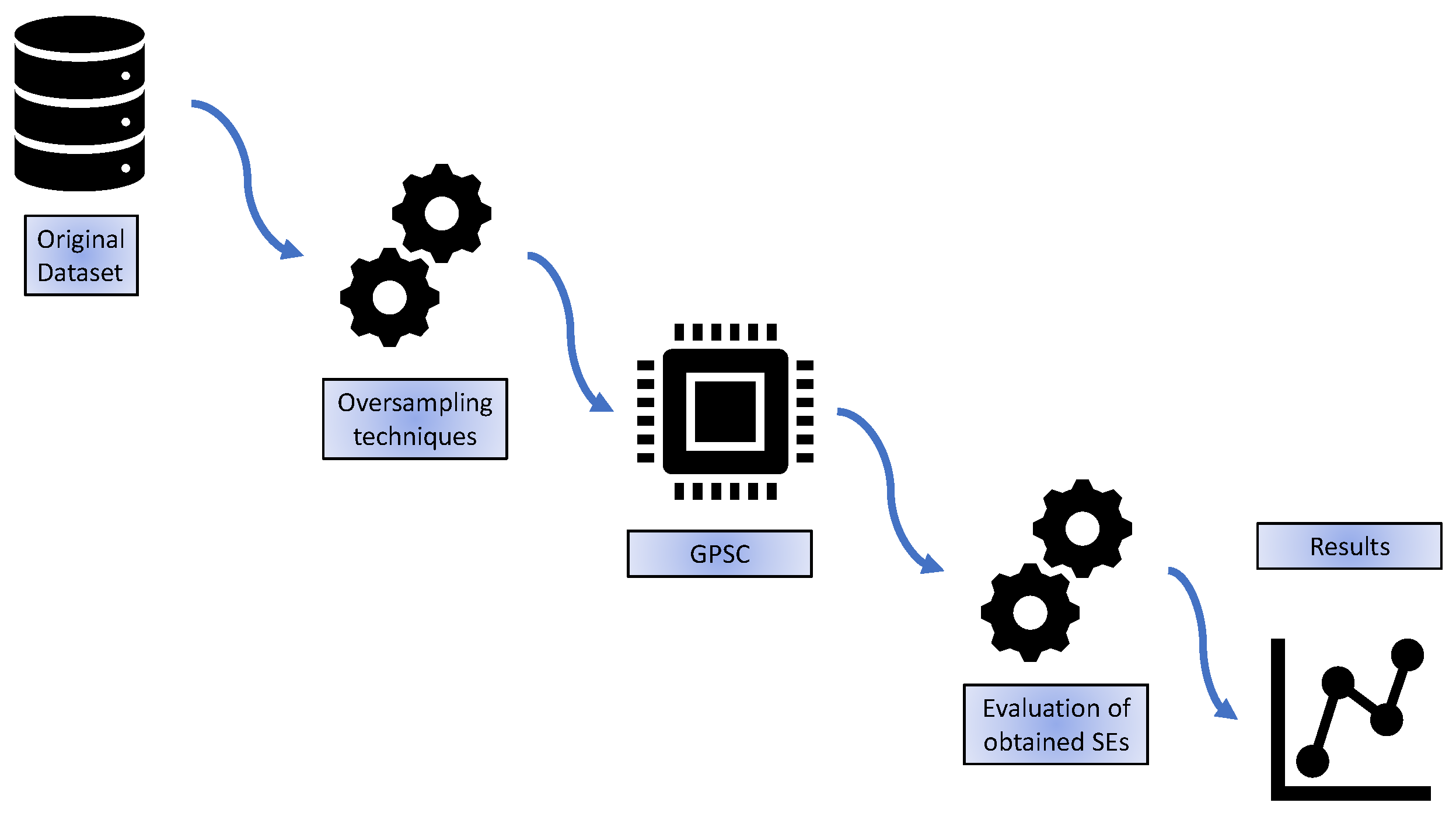
2.1. Research Methodology
- Original dataset—the initial investigation of the dataset is performed.
- Oversampling techniques—the idea is to apply various oversampling techniques to obtain balanced dataset variations from the original imbalanced dataset,
- GPSC—application of the GPSC algorithm with RHVS method on each dataset variation. For training of GPSC, the 5FCV method was used and if all evaluation metrics are greater than 0.99 then the final testing of obtained SEs is performed.
- Evaluation of obtained SEs—after GPSC + RHVS + 5FCV is applied on all dataset variations, all best SEs will be combined and evaluated on the original imbalanced dataset to see if the classification performance is the same/similar to the values obtained on the original imbalanced dataset.
- Results—presentation of obtained results on both balanced dataset variations and imbalanced original dataset.
2.2. Dataset Description
2.3. Oversampling Techniques
2.4. Genetic Programming Symbolic Classifier with Random Hyperparameter Value Selection
- PopSize—the size of the population.
- numGen—the maximum number of generations. This hyperparameter is one of the stopping criteria (in this investigation it was the dominating one).
- initDepth—the initial depth of population members when represented in the tree form.
- TourSize—the size of tournament selection. How many members will be randomly picked from the population to compete in tournament selection?
- Crossover—the probability of performing the crossover operation on the tournament winner. For this genetic operation, two tournament winners are needed and the subtree from one tournament winner is used and replaces the randomly selected subtree of the second tournament winner.
- subtreeMute—the probability of performing subtree mutation. This type of mutation begins by random selection of the subtree on the tournament winner. The second step is to create a subtree at random using constants, variables, and mathematical functions to produce a new subtree, thus creating a new population member.
- pointMute—the probability of performing the point mutation. It begins with a random selection of the tournament winner nodes which have to be replaced. The variables are replaced with other variables, constants with other constants, and mathematical functions with other mathematical functions. However, when these functions are replaced the new function must have the same number of variables as the original function.
- hoistMute—the probability of performing the hoist mutation of the tournament winner. This genetic operation begins by selecting a random subtree from the tournament winner and then selecting a random node (point) on that subtree. The randomly selected node replaces the entire randomly selected subtree.
- constRange—the range of constants arbitrarily defined.
- max samples—the max number of training samples used to evaluate population members in each generation. If the value is set to 1 then the raw fitness value is not visible during the GPSC execution, so the value is set between 0.99 and 1.
- ParsCoeff—this hyperparameter is very important since it regulates the use of the parsimony pressure method. This method is crucial during the GPSC execution to prevent the bloat phenomenon, i.e., the rise in the size of population members without any benefit to fitness function value. The parsimony pressure method is applied during the tournament selection in which large population members in terms of size are made less favorable for selection by multiplying their fitness value with the parsimony coefficient.
- Using values of input variables calculate the output of population member,
- Uses the generated output as input in the Sigmoid function which can be written as:where x is the output of the population member.
- Uses the output of the sigmoid function and the real output from the dataset to calculate the LogLoss value. The LogLoss according [] to is calculated using the following expression:where is the probability of 1, and is the probability of 0.
2.5. Training Procedure
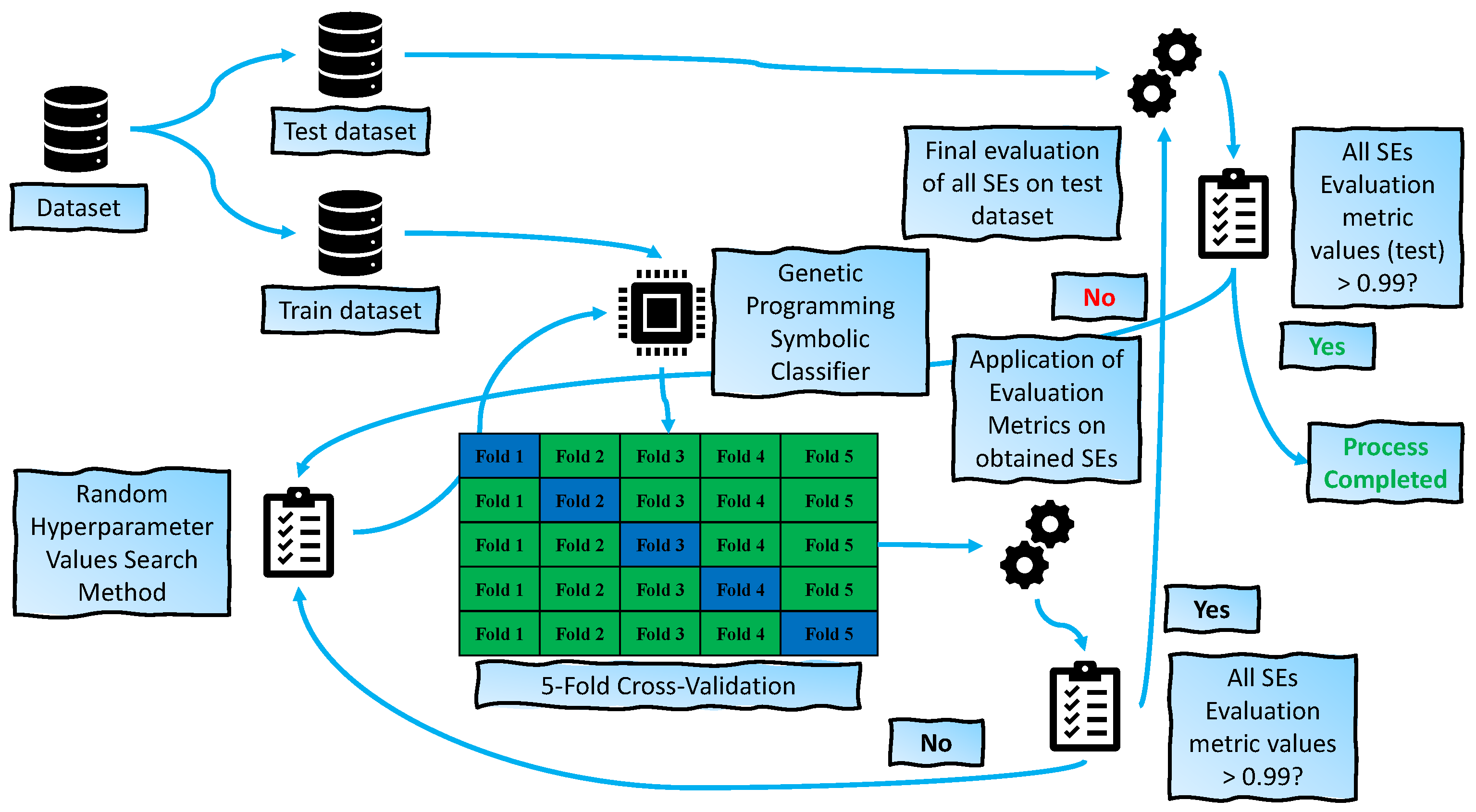
- The dataset (balanced dataset variation) was initially divided into training and testing datasets in a 70:30 ratio, where 70% was used for training using a 5-fold cross-validation process and the remaining 30% for testing. At this stage, the GPSC hyperparameters are randomly chosen from the predefined ranges.
- When the dataset is split into train and test datasets and the random hyperparameter values are chosen using the RHVS method, the training of the GPSC algorithm in the 5-FCV process can begin. In 5-FCV, the GPSC is trained 5 times, i.e., a total of 5 SEs are obtained after the 5-FCV process is completed. After the 5-FCV process is completed, the accuracy, area under the receiver operating characteristics curve, precision, recall, and f1-score values are obtained for training and validation folds. Then the mean and standard deviation of the previously mentioned evaluation metrics are calculated.
- All mentioned mean evaluation metric values have to be greater than 0.99 to be considered as the set of SEs with acceptable classification performance. If one of the evaluation metrics is lower than 0.99 in value, all the SEs are neglected and the process starts from the beginning, where random hyperparameters are randomly selected and GPSC training using the 5-FCV process is repeated. However, if all evaluation metric values are higher than 0.99, the process continues to the testing phase.
- In the testing phase, the remaining 30% of the dataset is used on all 5 SEs obtained from the previous step. Using the testing set in these 5SEs, the output is generated and compared to the real output to calculate the evaluation metric values. If all evaluation metric values are higher than 0.99, then the process is completed. However, if one evaluation metric value is lower than 0.99 the process starts from beginning by randomly selecting the hyperparameter values.
2.6. Evaluation Metrics
3. Results
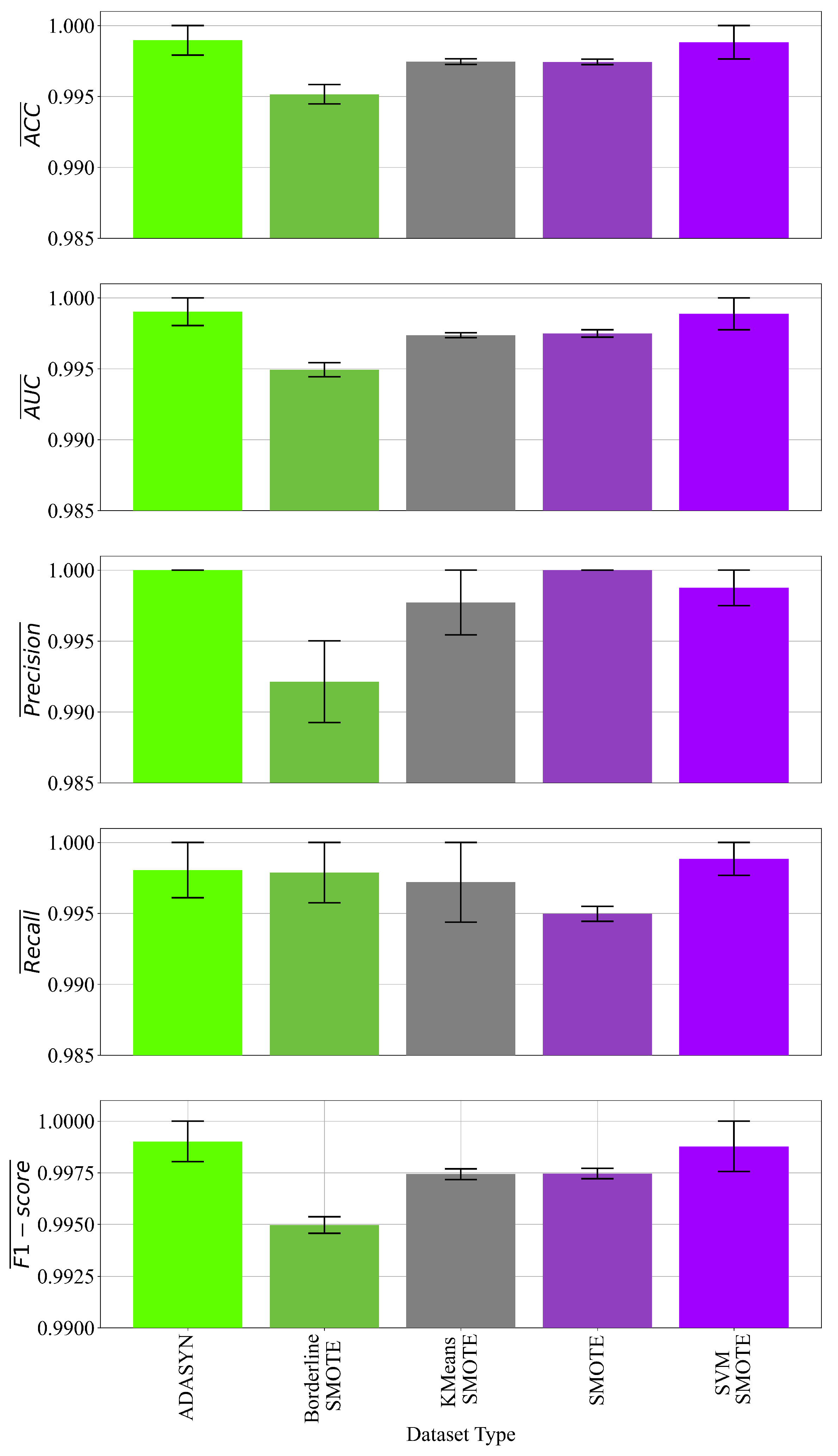
3.1. The Results Obtained on the Oversampled Datasets
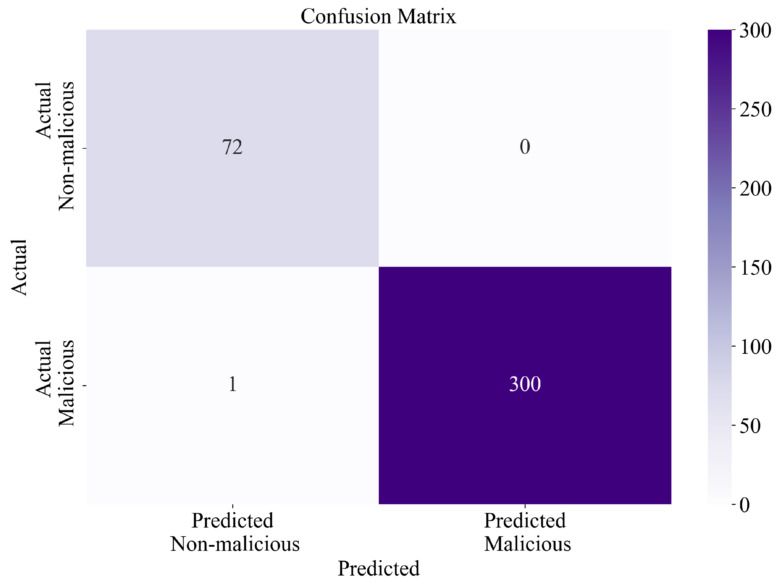
3.2. Classification Performance of Obtained Symbolic Expressions on the Original Dataset
4. Discussion
5. Conclusions
- The oversampling methods were successfully implemented and created balanced variations of the original dataset. However, in the case of ADASYN and KMeansSMOTE, the obtained versions of the dataset had an extremely small imbalance. This imbalance did not affect the classification performance of obtained SEs from these datasets.
- The application of GPSC was successful in obtaining the SEs with high classification performance in the detection of malicious software.
- Using the RHVS method, the optimal combination of GPSC hyperparameters were found for every application of GPSC on balanced dataset variation.
- A robust set of SEs with high classification performance was obtained for each dataset variation.
- Almost similar classification performance was achieved when all SEs were applied to the original imbalanced dataset, which proves that SEs were obtained with high classification accuracy. The further test revealed that only 1 out of 373 samples was misclassified.
- With the application of oversampling methods, the balanced variations of the original dataset were created, which is a good starting point for training any AI algorithm.
- With the application of GPSC, SEs are obtained that can be easily analyzed and integrated into other software.
- The application of the RHVS method proved to be useful in finding GPSC optimal hyperparameters, using which GPSC produced SEs with high classification performance.
- The application of 5FCV produced a set of SEs that are robust
- It takes a long time to train the GPSC algorithm and obtain SEs using the 5FCV process, i.e., the GPSC process is repeated for each split (it is repeated 5 times).
- The initial definition and testing of GPSC boundaries in the RHVS method is a challenging process that requires multiple GPSC executions.
- The search for optimal GPSC hyperparameter values using the RHVS method can take some time.
Author Contributions
Funding
Data Availability Statement
Conflicts of Interest
Appendix A
Appendix A.1. Modification of Mathematical Functions
Appendix A.2. How to Access and Use Obtained SEs
- Calculate the output by providing input dataset values,
- uses the output of each SE as the input in the Sigmoid function.
- After the values for the samples and all SEs are obtained calculate the accuracy score, area under receiver operating characteristics curve, precision score, recall score, and f1-score using functions defined in the python scikit-learn library.
References
- Alawida, M.; Omolara, A.E.; Abiodun, O.I.; Al-Rajab, M. A deeper look into cybersecurity issues in the wake of COVID-19: A survey. J. King Saud Univ.-Comput. Inf. Sci. 2022, 34, 8176–8206. [Google Scholar] [PubMed]
- Aslan, Ö.; Aktuğ, S.S.; Ozkan-Okay, M.; Yilmaz, A.A.; Akin, E. A comprehensive review of cyber security vulnerabilities, threats, attacks, and solutions. Electronics 2023, 12, 1333. [Google Scholar]
- Broadhurst, R. Cybercrime: Thieves, Swindlers, Bandits, and Privateers in Cyberspace. In The Oxford Handbook of Cyber Security; Oxford Handbooks Press: Oxford, UK, 2017. [Google Scholar]
- Li, B.; Zhao, Q.; Jiao, S.; Liu, X. DroidPerf: Profiling Memory Objects on Android Devices. In Proceedings of the 29th Annual International Conference on Mobile Computing and Networking, Madrid, Spain, 2–6 October 2023; pp. 1–15. [Google Scholar]
- Jain, M.; Bajaj, P. Techniques in detection and analyzing malware executables: A review. Int. J. Comput. Sci. Mob. Comput. 2014, 3, 930–935. [Google Scholar]
- Monnappa, K. Learning Malware Analysis: Explore the Concepts, Tools, and Techniques to Analyze and Investigate Windows Malware; Packt Publishing Ltd.: Birmingham, UK, 2018. [Google Scholar]
- Rauf, M.A.A.A.; Asraf, S.M.H.; Idrus, S.Z.S. Malware Behaviour Analysis and Classification via Windows DLL and System Call. J. Phys. Conf. Ser. 2020, 1529, 022097. [Google Scholar] [CrossRef]
- Narayanan, B.N.; Djaneye-Boundjou, O.; Kebede, T.M. Performance analysis of machine learning and pattern recognition algorithms for malware classification. In Proceedings of the 2016 IEEE National Aerospace and Electronics Conference (NAECON) and Ohio Innovation Summit (OIS), Dayton, OH, USA, 25–29 July 2016; pp. 338–342. [Google Scholar]
- David, B.; Filiol, E.; Gallienne, K. Structural analysis of binary executable headers for malware detection optimization. J. Comput. Virol. Hacking Tech. 2017, 13, 87–93. [Google Scholar] [CrossRef]
- Shaid, S.Z.M.; Maarof, M.A. In memory detection of Windows API call hooking technique. In Proceedings of the 2015 International Conference on Computer, Communications, and Control Technology (I4CT), Kuching, Malaysia, 21–23 April 2015; pp. 294–298. [Google Scholar]
- Rathore, H.; Agarwal, S.; Sahay, S.K.; Sewak, M. Malware detection using machine learning and deep learning. In Big Data Analytics, Proceedings of the 6th International Conference, BDA 2018, Warangal, India, 18–21 December 2018; Proceedings 6; Springer: Cham, Switzerland, 2018; pp. 402–411. [Google Scholar]
- Mahindru, A.; Sangal, A. MLDroid—Framework for Android malware detection using machine learning techniques. Neural Comput. Appl. 2021, 33, 5183–5240. [Google Scholar] [CrossRef]
- Vinayakumar, R.; Alazab, M.; Soman, K.; Poornachandran, P.; Venkatraman, S. Robust intelligent malware detection using deep learning. IEEE Access 2019, 7, 46717–46738. [Google Scholar] [CrossRef]
- Xu, Z.; Ray, S.; Subramanyan, P.; Malik, S. Malware detection using machine learning based analysis of virtual memory access patterns. In Proceedings of the Design, Automation & Test in Europe Conference & Exhibition (DATE), Lausanne, Switzerland, 27–31 March 2017; pp. 169–174. [Google Scholar]
- Piyush AnastaRumao. Using Two Dimensional Hybrid Feature Dataset to Detect Malicious Executables. Int. J. Innov. Res. Comp. Com. Eng. 2016, 4. [Google Scholar] [CrossRef]
- Fernández, A.; Garcia, S.; Herrera, F.; Chawla, N.V. SMOTE for learning from imbalanced data: Progress and challenges, marking the 15-year anniversary. J. Artif. Intell. Res. 2018, 61, 863–905. [Google Scholar] [CrossRef]
- He, H.; Bai, Y.; Garcia, E.A.; Li, S. ADASYN: Adaptive synthetic sampling approach for imbalanced learning. In Proceedings of the 2008 IEEE International Joint Conference on Neural Networks (IEEE World Congress on Computational Intelligence), Hong Kong, China, 1–8 June 2008; pp. 1322–1328. [Google Scholar]
- Han, H.; Wang, W.Y.; Mao, B.H. Borderline-SMOTE: A new over-sampling method in imbalanced data sets learning. In Advances in Intelligent Computing, Proceedings of the International Conference on Intelligent Computing, Hefei, China, 23–26 August 2005; Springer: Berlin/Heidelberg, Germany, 2005; pp. 878–887. [Google Scholar]
- Chen, Y.; Zhang, R. Research on credit card default prediction based on k-means SMOTE and BP neural network. Complexity 2021, 2021, 6618841. [Google Scholar]
- Almajid, A.S. Multilayer Perceptron Optimization on Imbalanced Data Using SVM-SMOTE and One-Hot Encoding for Credit Card Default Prediction. J. Adv. Inf. Syst. Technol. 2021, 3, 67–74. [Google Scholar] [CrossRef]
- Poli, R.; Langdon, W.B.; McPhee, N.F. A Field Guide to Genetic Programming; Lulu.com: Morrisville, NC, USA, 2008; 250p, ISBN 978-1-4092-0073-4. [Google Scholar]
- Anđelić, N.; Baressi Šegota, S. Development of Symbolic Expressions Ensemble for Breast Cancer Type Classification Using Genetic Programming Symbolic Classifier and Decision Tree Classifier. Cancers 2023, 15, 3411. [Google Scholar] [CrossRef] [PubMed]
- Sokolova, M.; Japkowicz, N.; Szpakowicz, S. Beyond accuracy, F-score and ROC: A family of discriminant measures for performance evaluation. In Advances in Artificial Intelligence, Proceedings of the Australasian Joint Conference on Artificial Intelligence, Hobart, Australia, 4–8 December 2006; Springer: Berlin/Heidelberg, Germany, 2006; pp. 1015–1021. [Google Scholar]
- McClish, D.K. Analyzing a portion of the ROC curve. Med. Decis. Mak. 1989, 9, 190–195. [Google Scholar] [CrossRef] [PubMed]
- Goutte, C.; Gaussier, E. A probabilistic interpretation of precision, recall and F-score, with implication for evaluation. In Advances in Information Retrieval, Proceedings of the European Conference on Information Retrieval, Santiago de Compostela, Spain, 21–23 March 2005; Springer: Berlin/Heidelberg, Germany, 2005; pp. 345–359. [Google Scholar]
- Susmaga, R. Confusion matrix visualization. In Intelligent Information Processing and Web Mining, Proceedings of the International IIS: IIPWM ‘04 Conference, Zakopane, Poland, 17–20 May 2004; Springer: Berlin/Heidelberg, Germany, 2004; pp. 107–116. [Google Scholar]


| Reference | ML Algorithms | Accuracy (%) |
|---|---|---|
| [11] | RFC, DNN-2,4,7 | 99.78 |
| [12] | SVM, RFC, MLP, LR, BN, AB, DT, KNN, DNN, SOM, FF, FC, DB, Y-J48, Y-SMO, Y-MLP, BTE, and MVE | 98.80 |
| [13] | LR, NB, KNN, DT, AB, RFC, SVM, CNN, MLP + SVM, and CNN + LSTM | 98.80 |
| [14] | LR, SVM, RFC | 100.00 |
| Dataset Variation | Class 0 Samples | Class 1 Samples | Total Number of Samples |
|---|---|---|---|
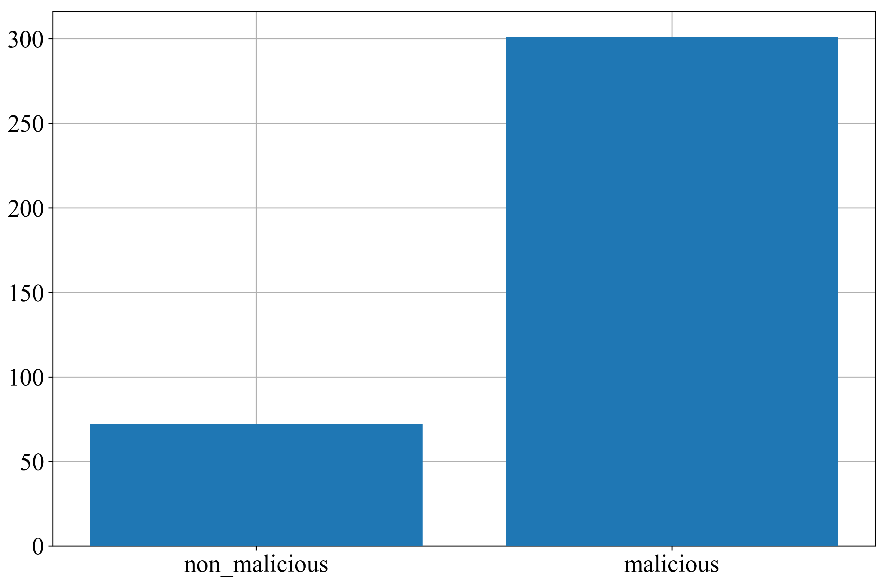
| Original dataset | 72 | 301 | 373 |
| ADASYN | 300 | 301 | 601 |
| BorderlineSMOTE | 301 | 301 | 602 |
| KMeansSMOTE | 304 | 301 | 605 |
| SMOTE | 301 | 301 | 602 |
| SVMSMOTE | 301 | 301 | 602 |
| Hyperparameter Name | Lower Boundary | Upper Boundary |
|---|---|---|
| PopSize | 1000 | 2000 |
| numGen | 200 | 300 |
| initDepth | 3 | 18 |
| TourSize | 100 | 500 |
| Crossover | 0.001 | 1 |
| subtreeMute | 0.001 | 1 |
| hoistMute | 0.001 | 1 |
| pointMute | 0.001 | 1 |
| constRange | −10,000 | 10,000 |
| max samples | 0.99 | 1 |
| ParsCoeff |
| Dataset Name | GPSC Hyperparameters |
|---|---|
| ADASYN | 1392, 175, 119, (7, 10), 0.0226, 0.96, 0.0093, 0.0061, , 0.995, (−9425.21, 4890.24), |
| BorderlineSMOTE | 1829, 168, 115, (3, 9), 0.0012, 0.96, 0.021, 0.01, , 0.993, (−9259.86, 3343.17), |
| KMeansSMOTE | 1943, 192, 120, (5, 12), 0.018, 0.96, 0.0047, 0.012, , 0.99, (−1423.02, 3973.33), |
| SMOTE | 1804, 187, 493, (4, 11), 0.031, 0.96, 0.004, 0.0032, , 0.996, (−4652.34, 3243.75), |
| SVMSMOTE | 1331, 187, 436, (4, 10), 0.0034, 0.95, 0.0093, 0.027, , 0.99, (−7067.54, 16.16), |
| Dataset Type | Depth of SEs | Length of SEs | Mean Depth | Mean Length |
|---|---|---|---|---|
| ADASYN | 13/17/12/22/13 | 52/169/95/91/92 | 15.4 | 99.8 |
| BorderlineSMOTE | 17/10/9/11/11 | 131/77/28/32/96 | 11.6 | 72.8 |
| KMeansSMOTE | 13/15/15/26/11 | 116/56/70/73/33 | 16.0 | 69.6 |
| SMOTE | 14/7/11/17/6 | 83/17/108/96/10 | 11 | 62.8 |
| SVMSMOTE | 20/20/9/22/19 | 112/38/32/55/88 | 18.0 | 65.0 |
| Evaluation Metric Name | Value |
|---|---|
| 0.9962 | |
| 0.0048 | |
| 0.9949 | |
| 0.0055 | |
| 0.9984 | |
| 0.0023 | |
| 0.9965 | |
| 0.0056 | |
| 0.9974 | |
| 0.0030 |
| Reference | ML Algorithms | Accuracy (%) |
|---|---|---|
| [11] | RFC, DNN-2,4,7 | 99.78 |
| [12] | SVM, RFC, MLP, LR, BN, AB, DT, KNN, DNN, SOM, FF, FC, DB, Y-J48, Y-SMO, Y-MLP, BTE, and MVE | 98.80 |
| [13] | LR, NB, KNN, DT, AB, RFC, SVM, CNN, MLP + SVM, and CNN + LSTM | 98.80 |
| [14] | LR, SVM, RFC | 100.00 |
| This research | Dataset balancing techniques + GPSC + RHVS + 5FCV | 99.62 |
Disclaimer/Publisher’s Note: The statements, opinions and data contained in all publications are solely those of the individual author(s) and contributor(s) and not of MDPI and/or the editor(s). MDPI and/or the editor(s) disclaim responsibility for any injury to people or property resulting from any ideas, methods, instructions or products referred to in the content. |
© 2023 by the authors. Licensee MDPI, Basel, Switzerland. This article is an open access article distributed under the terms and conditions of the Creative Commons Attribution (CC BY) license (https://creativecommons.org/licenses/by/4.0/).
Share and Cite
Anđelić, N.; Baressi Šegota, S.; Car, Z. Improvement of Malicious Software Detection Accuracy through Genetic Programming Symbolic Classifier with Application of Dataset Oversampling Techniques. Computers 2023, 12, 242. https://doi.org/10.3390/computers12120242
Anđelić N, Baressi Šegota S, Car Z. Improvement of Malicious Software Detection Accuracy through Genetic Programming Symbolic Classifier with Application of Dataset Oversampling Techniques. Computers. 2023; 12(12):242. https://doi.org/10.3390/computers12120242
Chicago/Turabian StyleAnđelić, Nikola, Sandi Baressi Šegota, and Zlatan Car. 2023. "Improvement of Malicious Software Detection Accuracy through Genetic Programming Symbolic Classifier with Application of Dataset Oversampling Techniques" Computers 12, no. 12: 242. https://doi.org/10.3390/computers12120242