
Classification of Wall Following Robot Movements Using Genetic Programming Symbolic Classifier


Faculty of Engineering, University of Rijeka, Vukovarska 58, 51000 Rijeka, Croatia
*
Author to whom correspondence should be addressed.
Machines 2023, 11(1), 105; https://doi.org/10.3390/machines11010105
Submission received: 23 December 2022
/
Revised: 10 January 2023
/
Accepted: 10 January 2023
/
Published: 12 January 2023
(This article belongs to the Special Issue Modeling, Sensor Fusion and Control Techniques in Applied Robotics)
Abstract
:The navigation of mobile robots throughout the surrounding environment without collisions is one of the mandatory behaviors in the field of mobile robotics. The movement of the robot through its surrounding environment is achieved using sensors and a control system. The application of artificial intelligence could potentially predict the possible movement of a mobile robot if a robot encounters potential obstacles. The data used in this paper is obtained from a wall-following robot that navigates through the room following the wall in a clockwise direction with the use of 24 ultrasound sensors. The idea of this paper is to apply genetic programming symbolic classifier (GPSC) with random hyperparameter search and 5-fold cross-validation to investigate if these methods could classify the movement in the correct category (move forward, slight right turn, sharp right turn, and slight left turn) with high accuracy. Since the original dataset is imbalanced, oversampling methods (ADASYN, SMOTE, and BorderlineSMOTE) were applied to achieve the balance between class samples. These over-sampled dataset variations were used to train the GPSC algorithm with a random hyperparameter search and 5-fold cross-validation. The mean and standard deviation of accuracy (), the area under the receiver operating characteristic (), precision, recall, and values were used to measure the classification performance of the obtained symbolic expressions. The investigation showed that the best symbolic expressions were obtained on a dataset balanced with the BorderlineSMOTE method with , , , , and equal to , , , , and , respectively. The final test was to use the set of best symbolic expressions and apply them to the original dataset. In this case the , , , , and are equal to , , , , , respectively. The results of the investigation showed that this simple, non-linearly separable classification task could be solved using the GPSC algorithm with high accuracy.
1. Introduction
Mobile robotics is an ever-growing field with a multitude of research focuses related to them [1]. Many applications of mobile robots can be seen today, such as transporting equipment [2], search and rescue [3], security [4], agriculture [5] and many others. One of the main issues of mobile robotics is the performance of its internal systems. Namely, the mobile robots in real word applications need to be real-time systems [6], which amongst other notable things, means that the performance of their internal systems-including all the calculations that need to be performed, has to be fast enough to allow for the real-time operation [7]. This can be achieved either by using a higher-performance controller machine for the mobile robot or by applying advanced algorithmic techniques to improve performance. One of the possible techniques is machine learning algorithms. These are data-driven methods that allow their internal parameters to be adjusted in the so-called training process [8]. During this process, the data points are used to tune the aforementioned internal parameters. This approach requires high-performance computers for the initial training—but once the model is finalized the exploitation of it to achieve results is usually extremely fast [9]. For this reason, and due to the high precision of the ML-generated models, a growing application of it for mobile robotics can be seen. Li et al. [10] discussed the possibility of applying data collected from human behavior for the training of AI-based methods. The authors showed that these methods can then be applied to the robots to complete tasks. Sevastopoulos and Konstantopoulos [11] showed that machine learning methods can be used to determine whether transversal of an area is possible. The authors demonstrated that the applied models can be used for the quick estimation of an area’s transversality. Eder et al. [12] demonstrated the use of machine learning for one of the key tasks in mobile robotics, which is the localization of the robots in space. The authors applied machine learning to identify the sensor particles, classifying them between noise and real measurements. Samadi Gharajeg and Jond [13] showed the application of fuzzy systems and supervised machine learning in mobile robotics. They applied the aforementioned methods to develop a speed controller for a leader-follower mobile robot.
One of the disadvantages of the previously described research is that after training, the artificial intelligence (AI) or machine learning (ML) model is obtained, which can be used for the classification of robot movements, but this model cannot be transformed into a simple mathematical equation. These trained models require additional computational resources for the storage and processing of new data from sensors.
The novel idea of this paper is to use a simple GPSC algorithm to obtain a set of symbolic expressions, which could based on the sensor data used for the detection of robot movements with high classification accuracy. The obtained symbolic expression does not require large computational resources when compared to other AI/ML algorithms and can be easily integrated into a control system of mobile robots as an additional tool for movement detection.
To obtain these symbolic expressions using the GPSC algorithm, a publicly available dataset [14,15] will be used, which contains data from 24 ultrasound sensors positioned on the wall following the robot. Since the original dataset is imbalanced, different balancing methods will be used to produce balanced dataset variations, which will be used to train the GPSC algorithm to obtain symbolic expressions. The process of obtaining the best symbolic expressions with the GPSC algorithm will be investigated by using a random hyperparameter search method with a 5-fold cross-validation process to obtain the optimal combination of GPSC hyperparameters, which will generate a robust set of symbolic expressions that could detect the robot movement with high classification accuracy.
Based on the previous research papers and the idea of this paper, the following questions arise:
- Is it possible to utilize the GPSC algorithm for the detection of the robot movement using data from ultrasound sensors with high classification accuracy?
- Does the dataset balancing methods have any influence on the classification accuracy of the obtained symbolic expressions using the GPSC algorithm?
- Is it possible to achieve the detection of the robot movement class with high classification accuracy using symbolic expressions that were obtained with the GPSC algorithm improved with the random hyperparameter search method and 5-fold cross-validation?
- Is it possible to achieve a similar classification accuracy of the best symbolic expression that was obtained using a balanced dataset on the original dataset?
The scientific contributions of this paper are:
- Investigate the possibility of implementing the GPSC algorithm on data collected from 24 ultrasound sensor data to detect the movement of the wall following robot;
- Investigate if the dataset balancing methods have any influence on the classification accuracy of the obtained symbolic expression using the GPSC algorithm;
- Investigate if the GPSC algorithm in combination with random hyperparameter search and 5-fold cross-validation can generate symbolic expressions with a high classification accuracy of robot movement detection, and;
- Investigate if the set of best symbolic expressions obtained on a balanced dataset variation can produce similar classification accuracy in robot movement detection when applied to the original dataset.
The outline of the paper can be divided into the following sections: Section 2, Section 3, Section 4, and Section 5. In Section 2, the research methodology, dataset with statistical analysis, dataset balancing methods, one versus rest classifier, GPSC algorithm, random hyperparameter search with 5-fold cross-validation, evaluation methodology, and used computational resources in this investigation are described. In the Section 3, the best results in terms of evaluation metric values are presented as well as the best set of symbolic expressions and the results obtained with the application of the best symbolic expressions on the original dataset. In the Section 4, the procedure used in this paper and the results are discussed. Based on the hypotheses defined in the Section 1 and Section 4, the conclusions are listed in the Section 5.
2. Materials and Methods
In this section, the research methodology will be described as well as dataset description with statistical analysis, genetic programming-symbolic classifier, random hyperparameter search method with 5-fold cross-validation, evaluation metrics, methodology, and computational resources, respectively.
2.1. Research Methodology
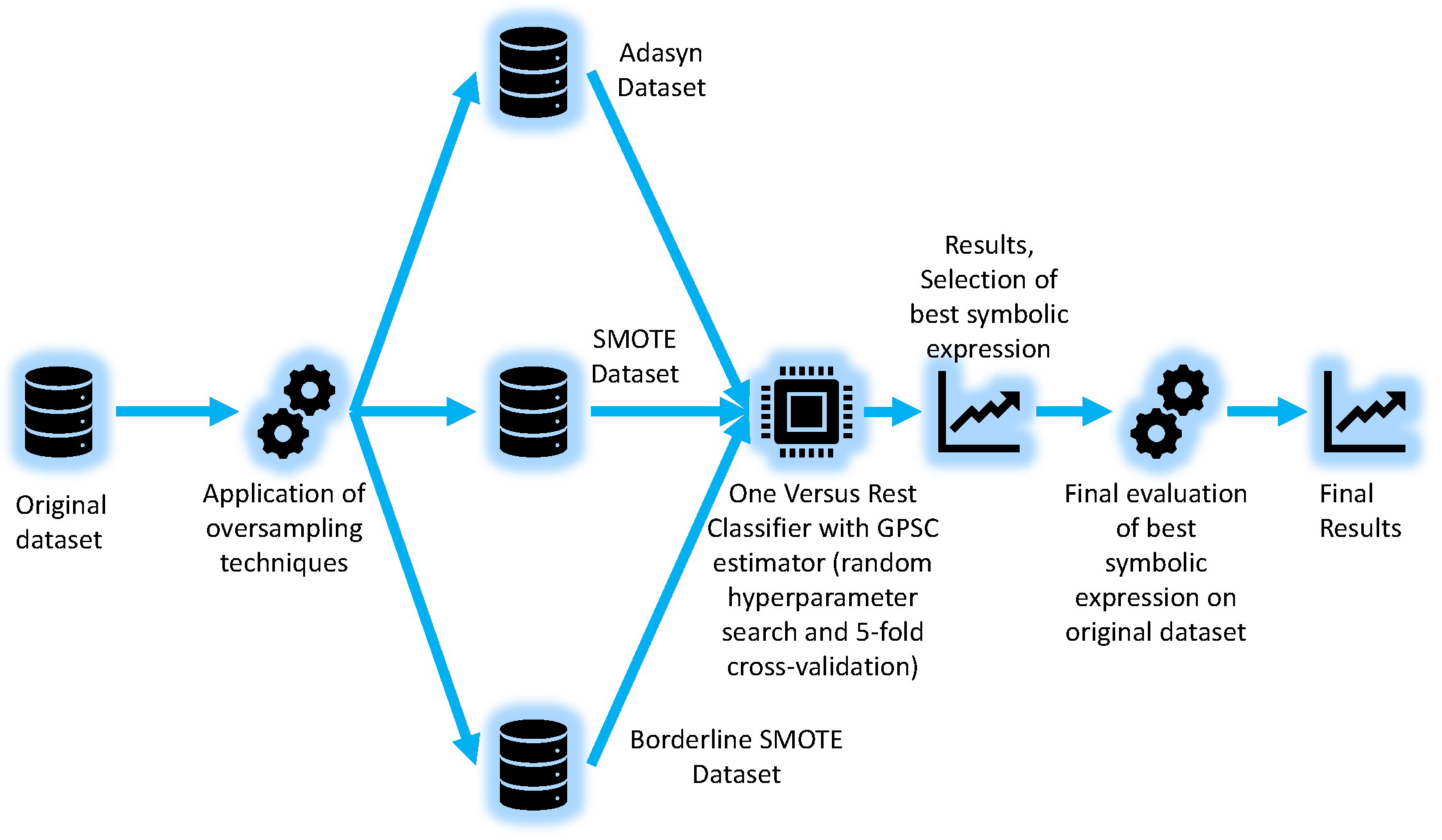
As already stated at the end of the Introduction section of this paper, the GPSC method will be utilized with a random hyperparameter search method and 5-fold cross-validation. However, since the original dataset is imbalanced, the oversampling methods will be applied to equalize the number of samples between all classes. When the symbolic expressions on each dataset variation were obtained, the best will be selected based on classification accuracy and the size of the symbolic expression in terms of length and depth. The best symbolic expression will be evaluated on the original dataset. The flowchart of the research methodology is shown in Figure 1.
As seen from Figure 1 the following oversampling methods were used to balance the dataset:
- Adaptive Synthetic (ADASYN);
- Synthetic Minority Oversampling (SMOTE);
- Borderline Synthetic Minority Oversampling (Borderline SMOTE) method.
These balancing methods equalized the number of samples between classes of the original dataset and were used in GPSC with random hyperparameter search and 5-fold cross-validation to obtain symbolic expressions with high classification accuracy. However, since there are four classes in the dataset, the One Versus Rest Classifier method has been used, where GPSC was the estimator. After the symbolic expressions were obtained, the selection of the best symbolic expression was performed by analyzing the highest classification accuracy and the size of the symbolic expression in terms of length and depth. The final evaluation of the best symbolic expression will be performed on the original dataset to obtain the classification accuracy.
2.2. Dataset Description
The dataset used in the research is a publicly available dataset titled “Sensor readings from a wall-following robot” [14,15]. The robot in question is the SCITOS G5 robot with 24 ultrasound sensors arranged around the robot’s midsection. There are a total of 5456 measurements. The measurement values of the individual sensor are stochastic and do not fit well with any common distribution. The descriptive statistics of the data are given in Table 1.
It can be seen that there is a decent amount of individually unique measurements for each of the sensor measurements, with 972 points at the lowest. When observing the combination of all the individual measurements, there are no duplicated values. Minimal sensor values are found in the range of 0.354 to slightly above 5.0. The upper value of that range is most likely the maximum value of the sensor measurement as it is consistent across the sensors. The average distances measured range between 1.254 and 3.201 without any general rule. The standard deviations of the dataset are high, indicating a good diversion of data in the dataset, which is a positive for the application of machine learning algorithms.
Before the use of the dataset for modeling, one final adjustment needs to be made. The classes are written textually as:
- “Move-Forward”;
- “Slight-Right-Turn”;
- “Sharp-Right-Turn”;
- “Slight-Left-Turn”.
However, the GPSC algorithm expects all the values to be numeric. The values in question are numerically encoded as 1 for “Move-Forward”, 2 for “Slight-Right-Turn”, 3 for “Sharp-Right-Turn”, and 4 for “Slight-Left-Turn”.
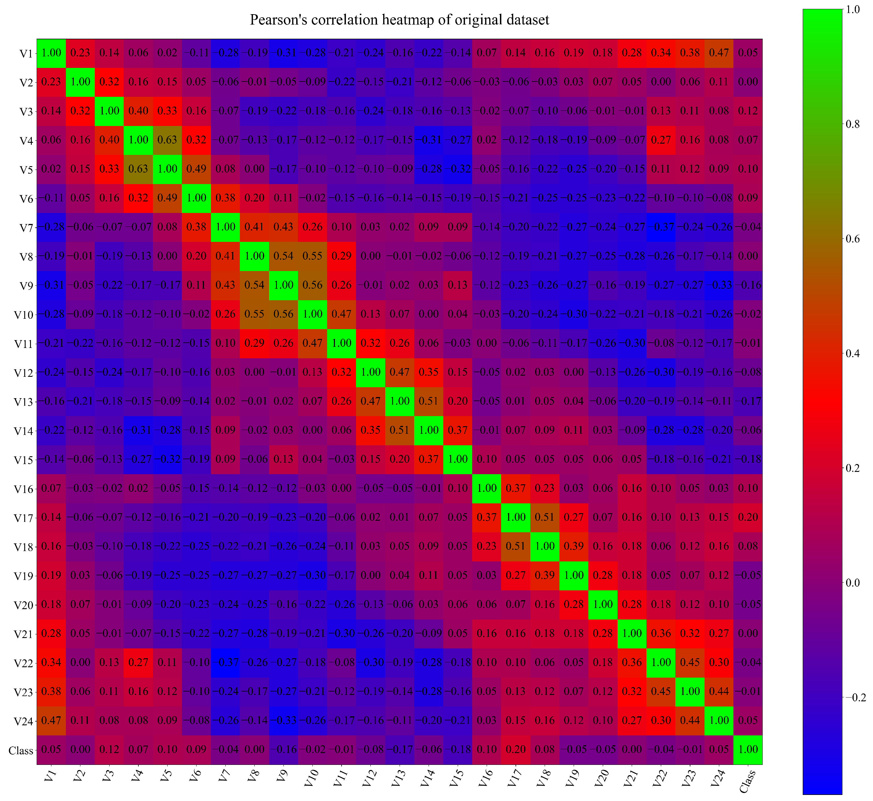
Another important factor in the statistical investigation of the dataset is correlation analysis. This correlation analysis provides information about the correlation between input variables and the target (output) variable. In this investigation, Pearson’s correlation analysis was used. The range of Pearson’s correlation is between −1.0 and 1.0. The value of −1.0 between one input variable and the target (output) variable means that if the value of the input variable increases, then the value of the output variable decreases, and vice versa. The correlation value of 1.0 between the input and output variables indicates that if the value of the input variable increases, then the value of the output variable will also increase. The 0 correlation value between the input and output variable indicates that, no matter if the value of the input variable increases or decreases, it will not influence the output variable. The results of Pearson’s correlation analysis are shown in the form of a heatmap in Figure 2.
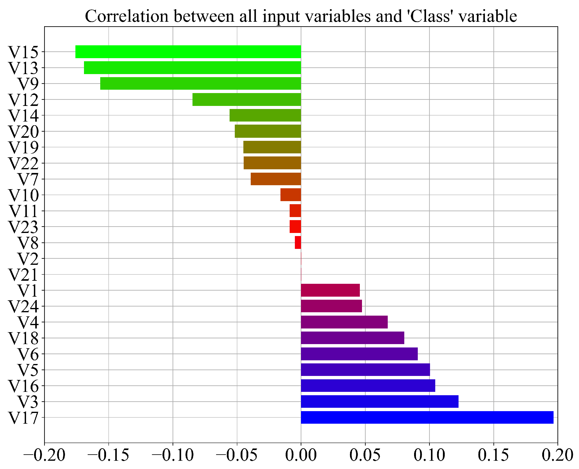
As seen from Figure 2 there are no highly correlated variables. The highest correlation is between the same variable. The range of correlation values between different variables is in the range between −0.3 and 0.5. To better visualize the correlation between all input variables (V1–V24) and the output (Class) variable, another correlation graph was created, which is shown in Figure 3.
As seen from Figure 3 the correlation between all input variables and the target ‘Class’ variable is in the −0.2–0.2 range. The highest correlation to the Class variable has the input variables V15, V13, V9, V3, and V17. Generally, the correlation analysis shows a low correlation between the input variables and output. However, all input variables will be used from the dataset in the GPSC algorithm to find symbolic expressions with high classification accuracy.
In the GPSC algorithm, the input variables will be presented from where , which are readings from ultrasound sensors placed at different positions while Class is the output (target) variable represented with y variable. In Table 2 the detailed description of each input variable and the GPSC variable representation are shown.
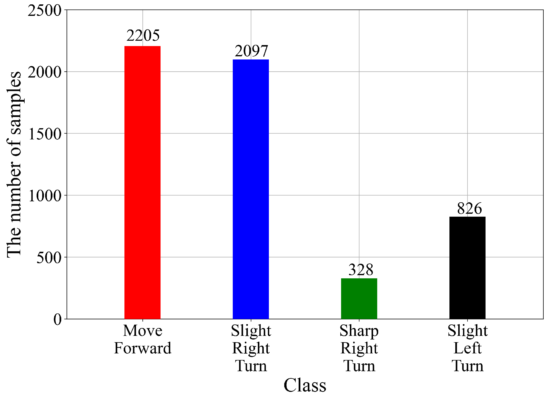
Before proceeding further, the number of samples per class should be investigated. The imbalanced dataset could result in poor classification performance of the ML models. As already stated in this dataset, there are four classes. The number of samples per class is shown in Figure 4.
As seen from Figure 4, the samples per class indicate that the dataset is highly imbalanced. The lowest number of samples is in the case of the Sharp-Right-Turn class (328), followed by Slight-Left-Turn (826), Slight-Right-Turn (2097), and Move-Forward (2205). The next step is to apply different oversampling methods to investigate if the dataset could be balanced. If the dataset is balanced, i.e., the number of samples per class is equal, then the GPSC algorithm could be applied. However, due to the small number of the third class (Sharp-Right-Turn) samples, the idea is to only apply oversampling methods.
2.3. Dataset Balancing Methods
In this paper, three different oversampling methods were used, i.e., ADASYN, SMOTE, and Borderline SMOTE. The undersampling methods were avoided because minority classes in the original dataset already contain a small number of samples, so further undersampling does not make any sense at all.
2.3.1. ADASYN
The Adaptive Synthetic (ADASYN) [16] method begins by identifying the number of samples in the majority () and minority () classes. The minority class is the class that has a low number of samples when compared to the number of samples of the majority class (), and the sum of both class samples must be equal to the total number of samples in the dataset (). To proceed in its execution, the ADASYN method must calculate the degree of class imbalance, which is the ratio between the minority and majority class samples, and in mathematical form can be written as:
The range of degree of class imbalance () is between 0 and 1.
To allow the ADASYN process to continue, the value must be below the predefined , which is a preset threshold for the maximum tolerated degree of class imbalance ratio. The next step is to calculate the number of synthetic data samples that have to be generated for the minority class, which is done using the expression:
where is the parameter for specifying the desired balance level after the generation of synthetic data. If is 1, a dataset will be balanced.
The next step is to find K nearest neighbors for each dataset sample that belongs to the minority class based on Euclidean distance in n dimensional space. After the K nearest neighbors of each sample from the minority class are found, the must be calculated using the following expression:
where is the number of samples in the K nearest neighbors of that belong to the majority class. The range of parameter is between 0 and 1. After the parameter is calculated it must be normalized so that is a density distribution ().
To calculate the number of synthetic data samples that have to be generated from each minority sample, the following expression is used:
where G (Equation (2)) represents the total number of samples that have to be generated for the minority class. The process of generating a synthetic data sample for each minority class data sample is done in two steps in each iteration. The range of the loop is from 1 to and the two steps are:
- Random selection of minority data sample from the KNN for data
- Generate the synthetic data sample using the following expression:where , and represent difference vectors in n-dimensional spaces and a random number in the 0 to 1 range, respectively.
2.3.2. Smote
The Synthetic Minority Oversampling Technique, according to Ref. [17], oversamples the minority class by taking each minority class sample and generating a synthetic sample along the line segments to join any or all K minority class nearest neighbors. The synthetic samples in SMOTE are generated in the following way:
- Calculate the difference between the sample and its nearest neighbor;
- Multiply the difference by a random number between 0 and 1 and add to the sample under consideration.
2.3.3. Borderline SMOTE
Borderline SMOTE, according to Ref. [18], begins its execution by calculating K nearest neighbors from the entire dataset for every in the minority class . If the majority of samples are found among the K nearest neighbors, they are denoted as K’. The second step is to investigate how many K’ are in K nearest neighbors and there are three possible combinations, i.e.,:
- K’ = K all the K nearest neighbors are majority samples;
- the number of majority neighbors is larger than the number of its minority ones. is considered to be easily misclassified and put into a DANGER set;
- the is excluded from further steps.
The collected samples in the DANGER set represent the borderline data of the minority class and the DANGER set can be defined as the subset of set.
The final step is to generate synthetic positive samples from samples in DANGER, where s is an integer in range 1 and k. For each sample in DANGER, a random nearest neighbor is selected from . The differences are calculated () between the sample from DANGER and the nearest neighbor from . Then the is multiplied with a random number in the 0 to 1 range. The synthetic minority sample is generated between the DANGER sample and its nearest neighbor using the equation, which can be written as:
where is a sample from the DANGER set.
After the application of previously described balancing methods to the original dataset, all minority classes (Slight-Right-Turn, Sharp-Right-Turn, and Sligth-Left-Turn) are successfully oversampled to reach the number of samples of the Move-Forward class. So, after the application of dataset oversampling methods, each class contains 2205 samples which are in total 8820 samples.
2.4. One Versus Rest Classifier
The one versus rest classifier [19] can be described as a heuristic method that is used for the application of binary classification algorithms in cases of multi-class classification. Using this method, the multi-class dataset is split into multiple classification problems. The binary classifier algorithm is then trained on each binary classification dataset and evaluations are made using the model that is most confident. The dataset used in this paper has four classes, i.e., “Move Forward” (1), “Slight-Right-Turn” (2), “Sharp-Right-Turn” (3), and “Slight-Left-Turn” as (4). The dataset can be divided into four binary classification datasets as follows:
- First Binary Classification Dataset: “Move Forward” vs. (“Slight-Right-Turn”, “Sharp-Right-Turn”, and “Slight-Left-Turn”);
- Second Binary Classification Dataset: “Slight-Right-Turn” vs. (“Move Forward”, “Sharp-Right-Turn”, and “Slight-Left-Turn”);
- Third Binary Classification Dataset: “Sharp-Right-Turn” vs. (“Move Forward”, “Slight-Right-Turn”, and “Slight-Left-Turn”);
- Fourth Binary Classification Dataset: “Slight-Left-Turn vs. (“Move Forward”, “Slight-Right-Turn”, and “Sharp-Right-Turn”).
The main disadvantage of this approach is that a GPSC classifier has to be created for each Binary Classification Dataset. In this case, four different GPSC models, i.e., symbolic expressions for four different datasets, are generated.
2.5. Genetic Programming-Symbolic Classifier
The execution of a Genetic programming-symbolic classifier (GPSC) starts with the creation of the initial population. To create the initial population, several hyperparameters have to be defined, i.e., population_size, number_of_generations, init_depth, functions, init_method, and constant_range. The population_size as the hyperparameter name states the size of the population that will be propagated through a specific number of generations defined with number_of_generations parameter. Each population member of the initial population is created by randomly selecting the constants from a predefined range of hyperparameter constant_range, mathematical functions from functions, and input variables from the dataset. The constantn_range is the range of constants values that GPSC randomly selects when creating the initial population and later in genetic operations (mutation). The list of mathematical functions used in this research consisted of addition, subtraction, multiplication, division, minimum, maximum, absolute value, square root, natural logarithm, logarithm with base 2 and 10, sine, cosine, tangent, and cube root. This mathematical function list is defined with hyperparameter functions. Since in GPSC, each population member is represented in tree form, the size of the tree is determined by the depth from the root node up to the deepest leaf of the tree. The depth of the tree is specified with hyperparameter init_depth. To explain the depth in detail, the mathematical equation in tree form is shown in Figure 5.
As seen from Figure 5 the root node is the “max” function, which is the 0 level of a tree node. At level 1, two mathematical functions are located, i.e., addition (“add”) and subtraction (“sub”). At final level 2, variables , , , and are located. So, this symbolic expression has init_depth of 2. To explain the procedure of defining the init_depth the method used to create the initial population must be explained first.
In all these investigations, the init_meth used to create the initial population is a ramped half-and-half method. This method creates the initial population using the full and growth method. The full method, according to Ref. [20], creates the initial population by taking the nodes at random from the function set until maximum tree depth is reached. Beyond the maximum depth, only variables and constants may be chosen. The problem with using only the full method to create the initial population is that all generated population members have trees with the same depth. The grow method, according to Ref. [20], creates the initial population by selecting functions, constants, and variables at random until the predefined depth limit is reached. Once this depth limit is reached, only variables and constants can be chosen. So, the growth method allows the creation of population members that have more varied sizes and shapes. The term ramped means that the depth of the symbolic expression had to be specified in a specific range, i.e., 3 to 12, which means that the population will have population members of depth between 3 and 12. The range is specified with init_depth hyperparameter.
After the initial population is created, the population members are executed and the output produced by each symbolic expression is stored. These outputs are then used in the Sigmoid decision function, which will produce an output. The Sigmoid decision function can be written in the following form:
This output is then used in the log loss function to compute how close it is to the corresponding actual value (0 or 1 in binary classification). So, the output of the log loss function is the prediction probability, which represents closeness to the actual output values of the dataset.
After the population members have been evaluated using the log loss fitness function, the tournament selection is applied to obtain the tournament winners on which the genetic operations will be applied to produce an offspring of the next generation. The population members that will enter each tournament selection is defined with tournament_size hyperparameter. So, in each generation, the specific number defined with tournament_size hyperparameter is randomly selected from the population and they are compared. The population member with the lowest value of fitness function (log loss value) and smallest size in terms of length and depth of symbolic expression (population member) is then selected as the winner of the tournament selection.
In this paper, on the winners of tournament selections, the four genetic operations were used, i.e., crossover, subtree mutation, hoist mutation, and point mutation to produce offspring of the next generation. The sum of these four operations should be near or equal to 1. If the sum is near 1 then some tournament selection winners might enter the next generation unchanged. On the other hand, if the value is equal to 1 then on all tournament selections the winners’ genetic operations will be applied. The crossover operation requires two tournament selection winners. On the first and second tournament selection winner, a random subtree is selected and the subtree from the second tournament selection winner replaces the three of the first tournament selection winner to generate offspring of the next generation. The subtree mutation requires one tournament selection winner and the random subtree on the winner is replaced with a randomly generated subtree, which is created by randomly choosing variables, constants, and mathematical functions. The hoist mutation requires one tournament selection winner and on this winner, a random subtree is selected and on that subtree, a random node is selected. Then, a random node replaces an entire subtree, i.e., the node is hosted in the position of the subtree. The point mutation randomly selects nodes on the tournament selection winner. The constants are replaced with other randomly chosen constants and variables with other variables. In the case of mathematical functions, the functions that are replacing other functions must have the same arity (same number of arguments).
The GPSC has two termination criteria that are controlled with two hyperparameters and these are number_of_generations and stopping_criteria value. The number of generations is the predefined number of generations for which GPSC is executed. After the last generation is reached, then the GPSC execution is terminated. The stopping criteria are the lowest value of the fitness function, in this the case log loss function, and if this value is reached by one of the population members before the maximum number of generations is reached, it will terminate the GPSC execution. However, in this investigation, the idea was to reach the lowest fitness function value possible so the stopping criteria were set in all investigations to an extremely small value, which means all GPSC executions were terminated after the maximum number of generations was reached.
During the execution of GPSC, the population members can grow rapidly from generation to generation without decreasing the fitness function value, i.e., the bloat phenomenon occurs. This phenomenon can negatively influence the execution time and can cause MemoryOverflow due to Computational resources. So, the large size of the population members can prolong the GPSC execution and can result in low classification performance. To overcome this problem, the parsimony method was used. In the parsimony pressure method during tournament selection, the fitness value of large population members is modified using the following expression:
where is the original fitness function of the population member, c is the parsimony coefficient, and is the size of the population member. So the new fitness function value is calculated by subtracting the product of the population member size and parsimony coefficient value from the original fitness value. Modifying the fitness function value of the population member makes them less favorable for selection, i.e., they will be less likely to be a tournament selection winner. The value of the parsimony coefficient in GPSC is regulated with pasimony_coefficient hyperparameter. This hyperparameter is one of the most sensitive hyperparameters, so initial tests are required to define its range. If the value is too large the method can prevent the evolution of population members and if the value is too small it can result in very large population members, i.e., very large symbolic expressions will be obtained with poor classification performance.
2.6. Random Hyperparameter Search with 5-Fold Cross-Validation
As stated in the estimator of OneVsRestClassifier, the GPSC algorithm is used with random hyperparameter search and 5-fold cross-validation. For this investigation, the random hyperparameter search method and 5-fold cross-validation had to be developed from scratch. However, before the development and implementation of random hyperparameter search, the initial investigation of the GPSC algorithm was performed to determine the ranges of specific hyperparameters such as population_size, number_of_generations, genetic operators, and parsimony_coefficient. The larger the population and the number of generations, the more time it will take to perform each GPSC execution. The genetic operations (crossover, subtree, hoist, and point mutation) differently contribute to the evolution process from generation to generation. The initial investigation found that the crossover value greatly influences the evolution process and lowers the fitness value from generation to generation. The most attention during the initial investigation was devoted to the parsimony coefficient since a large value can prevent evolution while a small value can lead to a bloat phenomenon. The GPSC hyperparameter ranges are listed in Table 3.
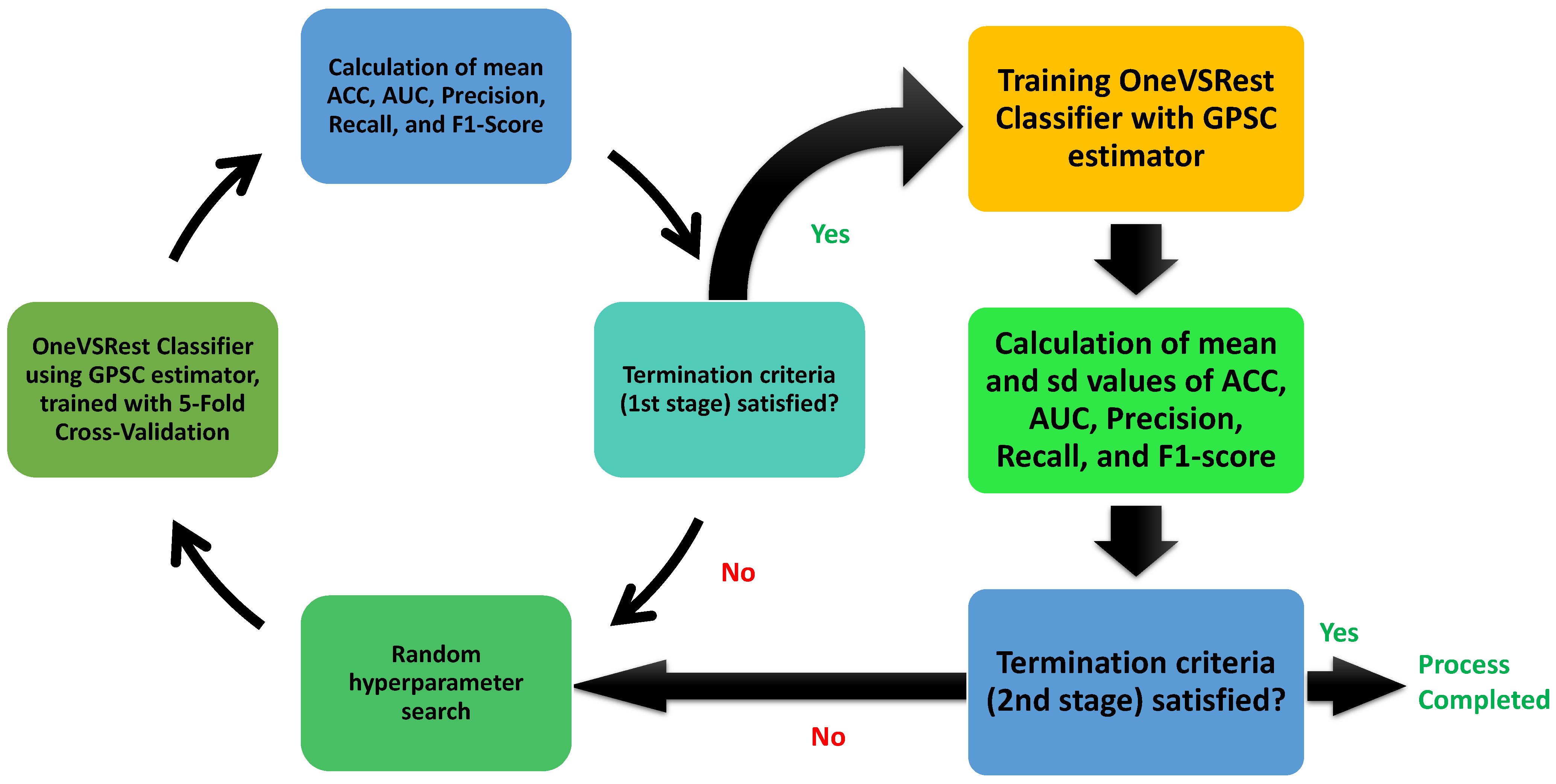
The GPSC hyperparameter ranges shown in Table 3 are defined after the initial investigation of the GPSC application on the dataset. The range of the population size hyperparameter range is large in order to ensure the large diversity in population and a large pool from which the population members will randomly be selected for tournament selection. In the initial investigation, the number of generations was below 200 and it was realized that a small maximum number of generations results in symbolic expressions with poor classification performance, so the maximum number of generation hyperparameters was set in the 200–300 range. Regarding the genetic operations, the crossover coefficient in the initial investigation was the most influential so its value for the random hyperparameter search method was set in the 0.95–1 range. The remaining three mutation operations occupy a small range between 0.95 and 1 and the starting condition of the GPSC execution is to ensure that the sum of all genetic operations is 0.999 or equal to 1. This is done because if the sum is lower than 1, then some of the tournament selection winners enter the next generation unchanged. The stopping criteria value or lowest log-loss fitness function value during GPSC execution was set to an extremely low value to stop the premature termination of GPSC execution. So, all GPSC algorithm executions in this investigation were terminated when the randomly selected maximum number of generations value is reached. The maximum number of samples hyperparameter range is the percentage of the training set used in each generation to evaluate the population members. The idea was to use the entire training dataset in the evaluation of each population member, so the value is set to the 0.99–1 range. The constant range was set to a specified range to ensure a large range from which GPSC will randomly pick numbers during the population initialization stage and later during the application of mutation operators. The most crucial hyperparameter was the parsimony coefficient, which is responsible for the prevention of the bloat phenomena. Since the correlation between input and output variables is pretty low, it is logical to assume that the GPSC will, during the execution, enlarge the size of population members to lower the fitness value, which can result in the bloat phenomenon. However, the initial investigation showed that the value of the parsimony coefficient has to be lowered to – range to ensure the growth of population members. Higher values of parsimony coefficients resulted in poor classification performance of obtained symbolic expressions. The entire procedure describing the random hyperparameter search method with 5-fold cross-validation is graphically shown in Figure 6.
The process starts with a random selection of the hyperparameters. This is followed by OneVsRestClassifier, in which the GPSC algorithm is the main estimator. The algorithm in question is trained using 5-fold cross-validation. After the training process is completed, then the mean values of accuracy (), the area under receiving operating characteristic curve (), , , and are calculated. If all the mean values are greater than 0.99, then the first stage of the process is complete and the next step is to perform a classic train/test using the same hyperparameters as was used previously. After training OneVsRestClassifer with the GPSC estimator, the obtained symbolic expressions were applied on the train and test dataset to calculate the mean and standard deviation values of , , , , and . If all mean values are greater than 0.99, then the process is terminated. It should be noted that standard deviation values are indications that overfitting did not occur. The large standard deviation value could indicate a large difference between the evaluation metric values achieved with the train and test datasets, respectively.
2.7. Evaluation Metrics and Methodology
In binary classification, after identifying the positive and negative classes with a trained ML model, the true positives, true negatives, false positives, and false negatives are defined. True positive is an outcome in which the trained algorithm correctly predicts the positive class. The true negative is an outcome in which the trained algorithm correctly predicts the negative class. The false positive is an outcome where the trained algorithm incorrectly predicts the positive class. The false negative class is an outcome where the trained algorithm incorrectly predicts the negative class.
The accuracy (), according to Ref. [21], can be described as the ratio between the number of correct predictions versus the total number of predictions. in mathematical form can be written as:
The area under the receiver characteristic operating curve [22] () is an evaluation metric that measures the ability of a classifier to distinguish between classes.
Precision [23] can be defined as the ratio between true positive and the sum of true and false positive. The precision is the ability of the trained classifier to not label a sample that is negative as positive. The formula for calculating precision can be written in the following form:
The recall [23] is the ability of the trained classifier to find all the positive samples. The recall is the ratio between true positive and the sum of true positive and false negative. The expression for calculating the recall can be written in the following form:
The harmonic mean of precision and recall is F1−Score. The formula for calculating the F1−score can be written as:
The value range of all the evaluation metrics used in this paper is between 0 and 1, where 1 represents the highest value of all evaluation metrics while the worst value is 0.
Since this is a multi-class problem, the OneVsRestClassifier was used with GPSC as the estimator. The evaluation metrics used can be applied to multi-class problems although this feature has to be specified when these metrics are called. Since all the datasets that were used for training and testing of GPSC are balanced, the macro option of , , , and was calculated. In the case of macro, the evaluation metric value is calculated for each class, and the unweighted mean is obtained. This method does not take class imbalance into account and, since all datasets are balanced, this is the perfect method.
2.8. Computational Resources
In this paper, all investigations were conducted on a desktop computer with an Intel CPU i7 4770 with 16 GB of DDR3 RAM. All program codes were written in Python Programming Language (version 3.7). The dataset was balanced with help of imblearn library (v. 0.9.0). The OneVsRestClassifier, as well as evaluation metrics, were imported from the sklearn library (V.1.12). The GPSC algorithm was imported from the gplearn library (v.0.4.0). The random hyperparameter search method was built from scratch using Python random library to randomly select each hyperparameter from the prespecified range, which is shown in Table 3. The 5-fold cross-validation was also built from scratch with procedures for exporting and cleaning symbolic expressions.
3. Results
In this section, the results of the conducted investigation were shown. First, the results obtained on each dataset variation were presented in terms of evaluation metrics, size of symbolic expressions (length), and average CPU time required to obtain the solution. Then based on the detailed analysis, the best set of symbolic expressions is presented and finally evaluated on the original dataset.
3.1. The Classification Performance of Symbolic Expressions Obtained for Each Dataset Variation
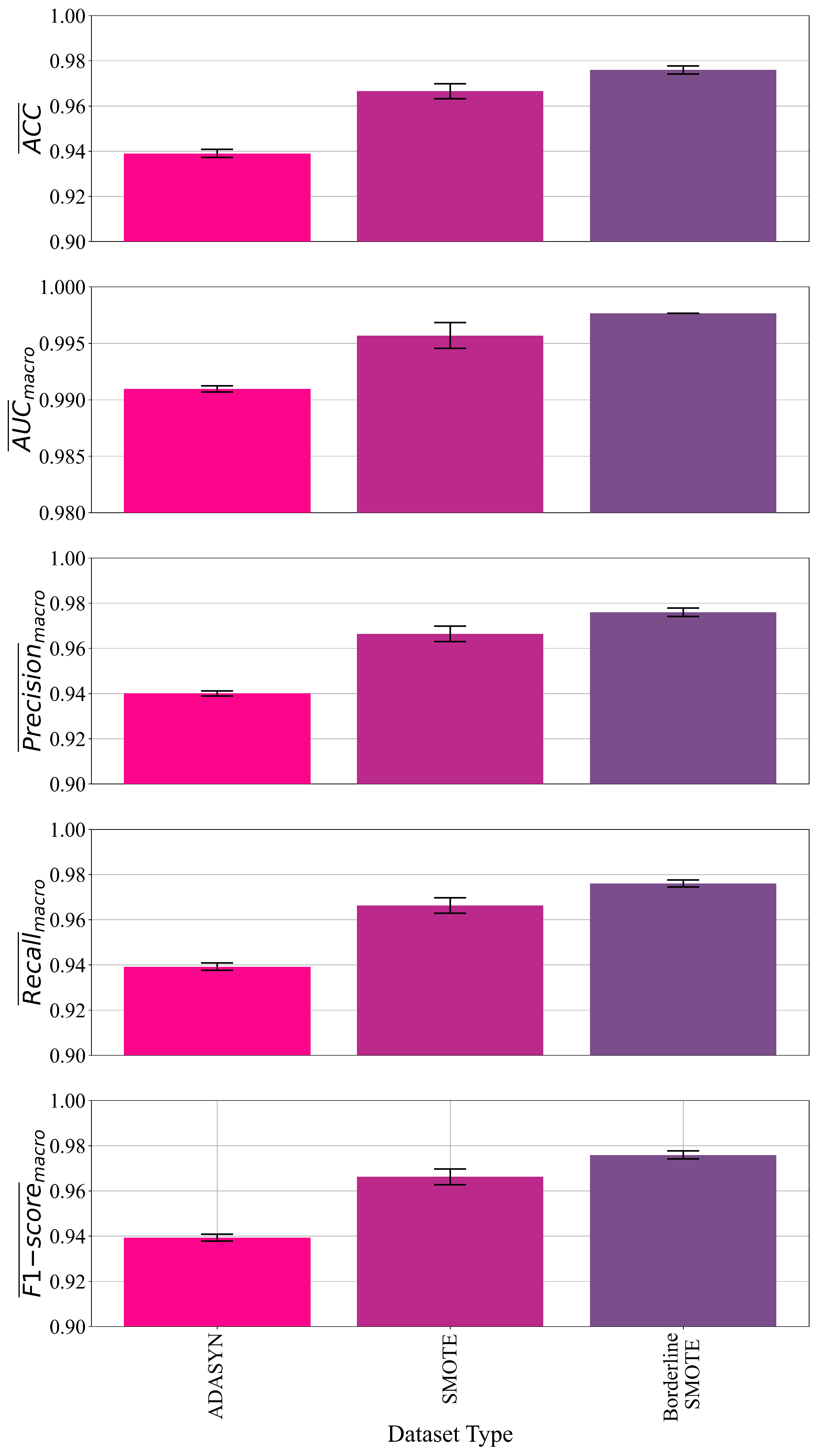
The results of a conducted investigation using OneVSRestClassifier with GPSC estimator, random hyperparameter search, and 5-fold cross-validation are shown in Figure 7, and Table 4. The results are presented in a table format due to the small standard deviation values shown as error bars in Figure 7 and, besides that, some additional information about the length of symbolic expressions as well as the average CPU time that was required to obtain the symbolic expressions are given. The hyperparameters used to obtain these symbolic expressions are shown in Table 5 for each dataset variation.
As seen in Figure 7 the best classification accuracy was obtained in the case where the GPSC algorithm was trained on the dataset balanced with the BorderlineSMOTE method followed by the symbolic expressions obtained on datasets balanced with SMOTE and ADASYN methods. The standard deviation values represented as error bars are fairly small, which indicates that overfitting did not occur during the training of the GPSC algorithm. In Table 4 the mean and standard deviation values of the evaluation metrics are shown for each dataset variation, and from these values, it can be seen that standard deviation values are in – range.
The average CPU time required to obtain the set of four symbolic expressions for the detection of robot movement of the wall-following robot is equal to 2400 [min] regardless of the dataset variation on which the GPSC algorithm was trained. Since this is a multi-class problem and OneVsRestClassifier was used with GPSC algorithm and 5-fold cross-validation, the total number of GPSC executions for a set of randomly chosen hyperparameters (one value for each hyperparameter) is 24. There are four classes and for each class, 5-fold cross-validation was performed. After the process of 5-fold cross-validation for each class is done, the mean values of evaluation metrics were computed and if they are greater than 0.95, then the final train/test is performed. In this final stage, each class is trained on the train part of the dataset to obtain symbolic expression. Since there are four classes, this final stage is repeated 4 times. So, there are 20 GPSC algorithm executions in the 5-fold cross-validation process and 4 additional GPSC algorithm executions in the final train/test, which equals in a total if 24 GPSC algorithm executions. The average CPU time for one GPSC algorithm execution is 100 [min], so the total average CPU time required to obtain a set of 4 symbolic expressions (one symbolic expression per class) for one set of randomly chosen hyperparameters is equal to 2400 [min].
The length of the symbolic expression is measured in the number of elements (mathematical functions and variables) that the symbolic expression contains. From Table 4 it can be noticed that the size of symbolic expressions regardless of the dataset variation on which they obtained is large. The best symbolic expressions in terms of classification accuracy are obtained on the dataset balanced with the BorderlineSMOTE method. The smallest symbolic expressions in terms of length were obtained in the case of the dataset balanced with the SMOTE method however, the classification performance is lower than in the case of BorderlineSMOTE dataset variation. The symbolic expressions obtained on the dataset balanced with the ADASYN method achieved the lowest classification performance, and the length of these symbolic expressions is slightly higher than those obtained in the case of SMOTE dataset.
The symbolic expressions obtained in the case of the BorderlineSMOTE dataset are chosen as the best symbolic expressions. Although these expressions are very large they achieved the highest classification accuracy with a small standard deviation, which indicates that overfitting did not occur. The reason why these expressions were chosen is the assumption that if they achieved the highest classification accuracy on a balanced dataset, then they will most likely achieve similar results on the original imbalanced dataset since imbalanced datasets have a huge influence on classification performance on ML models in general.
The best symbolic expressions for each case were obtained with a GPSC algorithm with the combination of randomly chosen hyperparameter values that are listed in Table 5.
From Table 5 it can be noticed that the population size, crossover, and the maximum number of samples hyperparameters are similar in all three cases. In the case of the BorderlineSMOTE dataset, the parsimony coefficient is the lowest, which contributed to the size of generated symbolic expressions; however, these symbolic expressions achieved the highest classification accuracy.
The best symbolic expressions that are obtained on the BorderlineSMOTE dataset will be presented and evaluated on the original imbalanced dataset in the next subsection.
3.2. The Best Set of Symbolic Expressions and Final Evaluation
Based on the obtained results, the best set of symbolic expressions was obtained in the case of the BorderlineSMOTE dataset. Since there are four equations in the set, each symbolic expression is used to detect a specific class, i.e., the first expression for the detection of the “Move-forward” (1) class, the second expression for the detection of the “Slight-Right-Turn” (2) class, the third for detection of the “Sharp-Right-Turn” (3) class, and finally the fourth expression for detection of the “Slight-Left-Turn” (4) class. The set of best symbolic expressions obtained in the case of the dataset borderlineSMOTE method can be written in the following form given in the Appendix A.
Looking at Equations (A1)–(A4) they are very large. However, after close inspection, each equation contains a different combination of input variables, i.e., readings from ultrasound sensors. The Equation (A1) is used to detect the “Move-Forward” (class value 1) motion of the wall following the robot. The equation consist of , , , , , , , , , , and variable. These input variables (Table 2) are readings from ultrasound sensors placed at angles −165°, −150°, −120°, −105°, −90°, −60°, 0°, 30°, 75°, 105°, and 120°, respectively. The Equation (A2) is used to detect the “Slight−Light−Turn” (class value 2) motion of wall following robot and consists of , , , , , , , , , , , and variable. These input variables (Table 2) are readings from ultrasound sensors placed at angles: −165°, −150°, −135°, −75°, −60°, −15°, 0°, 15°, 30°, 45°, 75°, and 90°, respectively. The Equation (A3) is used to detect the “Sharp−Right−Turn” (class value 3) motion of the wall following robot and consists of , , , , , , , , and variable. Looking at Table 2 these input variables are readings from ultrasound sensors at reference angles −180°, −165°, −150°, −75°, −15°, 15°, 30°, and 60°, respectively. The final Equation (A4) is used to detect the “Slight−Left−Turn” (class value 4) motion of the wall following robot and consists of , , , , , , , , , , , , , and variable. From Table 2 these input variables represent readings from ultrasound sensors at the following reference angles: −165°, −150°, −135°, −90°, −60°, −45°, −30°, −15°, 0°, 30°, 60°, 90°, and 135°, respectively.
It is interesting to notice that each symbolic expression does not require all 24 readings from ultrasound sensors. The Equation (A3) requires readings of 9 ultrasound sensors to compute the output followed by the Equations (A1), (A2) and (A4) that require 11, 12, and 14 ultrasound sensors. The final evaluation of the best symbolic expression will be performed on the original dataset and, to evaluate these expressions, the following steps are:
- Calculate the output of each symbolic expression using original dataset values;
- Use this output in the Sigmoid function to generate the output;
- Transform the obtained output into integer form for each symbolic expression, and;
- Compare the obtained results with the original output and calculate the evaluation metric values.
The results of evaluating the best symbolic expressions obtained in the case of the dataset balanced with the BorderlineSMOTE method on the original dataset are shown in Table 6.
To obtain the mean and standard deviation of evaluation metric values shown in Table 6 the output of each symbolic expression is calculated and used in the Sigmoid decision function to compute the output (in integer form). Then this output is compared to the output from the original dataset and , , , , and were computed for each symbolic expression. After these values were obtained, the mean and standard deviation values were calculated. As seen from Table 6 the evaluation metric values showed that the set of best symbolic expressions achieve slightly lower classification accuracy on the original dataset than on the dataset on which they were obtained (BorderlineSMOTE dataset).
4. Discussion
Initial correlation analysis showed that all input variables have a low correlation with the output (target) variable (Figure 2). The correlation values are in the −0.2 to 0.2 range (Figure 3). However, to investigate which input variables will end up in the best symbolic expressions, all input variables were used for training the GPSC algorithm.
Since the original dataset is highly imbalanced, three different balancing methods were applied: ADASYN, SMOTE, and BorderlineSMOTE. These methods equalized the number of samples per class by oversampling three minority classes. Using these three balancing methods, three different dataset variations were obtained.
On each dataset variation, the OneVsRest classifier was applied with the GPSC algorithm as the classifier estimator and was trained using a 5-fold cross-validation method. The random hyperparameter search method was used to find the combination of hyperparameters used, which for each class used the symbolic expression with the highest classification accuracy obtained.
Before implementing the previously described procedure, the initial investigation was conducted to define the ranges of each hyperparameter from which the hyperparameters will be randomly selected before each GPSC algorithm execution. The most sensitive hyperparameter was the parsimony coefficient, which is responsible for the prevention of the bloat phenomenon. As seen from Table 5 the best symbolic expressions obtained on each dataset variation had a very large population, which was propagated through 100 to almost 300 generations. The stopping criteria value in all investigations was never met, since the idea was to terminate the GPSC execution when a maximum number of generations was reached. The dominating genetic operation in all investigations was crossover, since in the initial investigation used for the development of the random hyperparameter search method it was noticed that this genetic operation is the most influential.
The parsimony coefficient in all investigations is low to ensure the growth of the population members. Since the correlation between dataset variables is low, the size of the symbolic expressions grew from generation to generation, intending to lower the fitness function value. The bloat phenomenon did not occur since the fitness function value was successfully lowered from generation to generation which resulted in the symbolic expressions with high classification performance. The best set of symbolic expressions is large due to the low correlation between the variables; however, the classification accuracy is high.
The best set of symbolic expressions was obtained on the dataset balanced with the BorderlineSMOTE method. The implementation of random hyperparameter search with a 5-fold cross-validation method produced symbolic expressions with high mean values of evaluation metrics and small standard deviation values, which indicates that overfitting did not occur. The investigation showed that the symbolic expressions do not require all input variables from the dataset. From 24 input variables in the dataset, 9 input variables are required for the detection of “Move-Forward” movement, 11 input variables are required to detect “Slight-Right-Turn” movement, 12 input variables are required to detect “Sharp-Right-Turn” movement, and 14 input variables are required to detect the “Slight-Left-Turn” movement.
The final test of implementing the set of symbolic expressions on the original imbalanced dataset showed that slightly lower classification performances were achieved when compared to the classification performance achieved on the BorderlineSMOTE dataset.
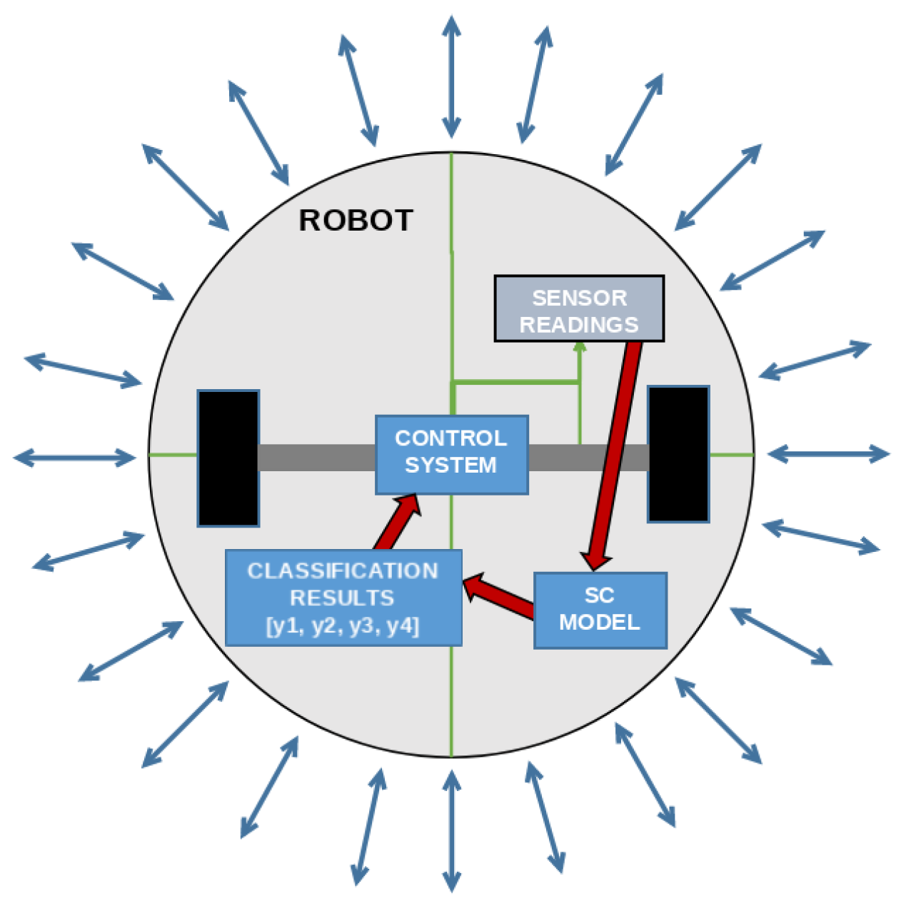
The achieved models could be used in the manner shown in Figure 8. The data collected from the 24 sensors positioned around the mobile robot is collected to the sensor bus (marked with “Sensor readings”). This data is then transferred to an internal computation device at which the achieved models, as presented in equations, have been stored. This process will return a vector of possible classes, in which one will be near equal to 1.0 due to the application of the sigmoid function, while the other will be near zero, for the same reason. This vector is then passed to the control system, which will actuate the motors which constitute the movement system of the robot in such a manner as to achieve the expected movement (forwards, slight or sharp right turn, or slight left turn). The pseudocode showing this implementation is given in Appendix B.
5. Conclusions
In this paper, the OneVSRestClassifier was applied with GPSC estimator, random hyperparameter search, and 5-fold cross-validation on the publicly available dataset to obtain symbolic expressions, using the detection/classification of the robot movement with sensor readings as the output, with high classification accuracy. Since the original dataset is imbalanced, oversampling methods (ADASYN, SMOTE, and BorderlineSMTOE) were used to balance the dataset (equalizing the number of samples per class). These balanced dataset variations were used to obtain symbolic expressions and the set of best symbolic expressions was evaluated on the original imbalanced dataset. The methods, such as the one explored in this paper, have a wide possibility of applications due to the generated format. A large amount of data is generated during the use of various robotic systems, thanks to the sensors that exist in such systems [24]. This allows for the application of machine learning methods in various robot-based systems, such as telemedicine [25], remote sampling [26], human–robot collaboration [27], and others. Based on the conducted investigation, the following conclusions are:
- The GPSC algorithm successfully generated the symbolic expressions, which can be used for the detection/classification of the robot movement with high classification accuracy;
- The dataset balancing method (ADASY, SMOTE, and BorderlineSMOTE) balanced the original dataset and provided a good starting point for the training of the GPSC algorithm, which resulted in symbolic expressions with high classification accuracy. So the investigation showed that dataset balancing methods have a great influence on the classification accuracy of the obtained symbolic expressions;
- The GPSC algorithm with the random hyperparameter search method and 5-fold cross-validation proved to be a powerful tool in obtaining robust and highly accurate symbolic expressions;
- The investigation showed that the best set of symbolic expressions obtained on a dataset balanced with the oversampling method can be applied to the original dataset and achieve high classification accuracy. This shows the validity of the proposed method;
- The procedure showed that a dataset with a low correlation between variables can be used to obtain symbolic expressions with GPSC and that these symbolic expressions do not require all the input variables to classify the movement of the robot.
The advantages of the approach are:
- Using the proposed method, symbolic expressions are obtained, which are easier to use and understand in comparison to ML models, and require less computational resources for storage and processing than other ML-trained models;
- The oversampling methods can balance the dataset and, by using these datasets, the classification accuracy can be improved;
- Random hyperparameter search and 5-fold cross-validation are useful tools for obtaining robust solutions with high classification accuracy,
The disadvantages of the approach are:
- The initial hyperparameter range definition is a painstaking process as the range of each hyperparameter has to be tested. Special attention must be paid to the parsimony coefficient value since this parameter is the most sensitive. Small values can result in a bloat phenomenon, while large values can result in obtaining symbolic expressions with low classification accuracy;
- Regardless of the computational resources used, the execution of GPSC can be a time-consuming process especially if the correlation between input variables is low. If the correlation values between variables are low, GPSC will try to minimize the fitness function value by enlarging the population member’s size, which can in some cases result in the bloat phenomenon.
Another limitation of the article that must be noted is the lack of verification on a real robot. This would serve as further proof of the achieved performance. The current level of validation on existing data should be of a satisfactory level for a proof-of-concept, indicating the possibility of using equations generated via a symbolic classifier for robot movement. The aforementioned real-life validation may be part of future work, especially in combination with an online training system for the further tuning and improvement of the achieved models. Future work may also be focused on obtaining symbolic expressions that are smaller in size and have higher classification accuracy than those presented in this paper. This will be achieved by using different synthetic data generation methods, which can in some cases improve the correlation between input variables. One of the ideas for future work is to obtain the original dataset by using data from multiple sensors that are positioned on the mobile robot.
Author Contributions
Conceptualization, N.A. and I.L.; data curation, N.A. and S.B.Š.; formal analysis, I.L. and M.G.; funding acquisition, N.A. and M.G.; investigation, S.B.Š.; methodology, N.A. and S.B.Š.; project administration, M.G.; resources, M.G.; resources, M.G.; software, N.A.; supervision, I.L. and M.G.; validation, I.L.; visualization, S.B.Š.; writing—original draft, N.A. and S.B.Š; writing—review and editing, I.L. and M.G. All authors have read and agreed to the published version of the manuscript.
Funding
This research received no external funding.
Institutional Review Board Statement
Not applicable.
Informed Consent Statement
Not applicable.
Data Availability Statement
The data used in this paper was obtained from a publicly available repository located at https://www.kaggle.com/datasets/uciml/wall-following-robot, accessed on 9 January 2023.
Acknowledgments
This research has been (partly) supported by the CEEPUS network CIII-HR-0108, European Regional Development Fund under the grant KK.01.1.1.01.0009 (DATACROSS), project CEKOM under the grant KK.01.2.2.03.0004, Erasmus+ project WICT under the grant 2021-1-HR01-KA220-HED-000031177, and University of Rijeka scientific grant uniri-tehnic-18-275-1447.
Conflicts of Interest
The authors declare no conflict of interest.
Appendix A
This appendix contains the best performing equations obtained using the methods described in the main body of the paper.
Appendix B
This section contains the pseudocode for the proposed control algorithm based on the classification equations obtained using the described methodology (given in the Appendix A).
| Algorithm A1 An algorithm with caption | |
▹ Define the vector for sensor readings of length 24 | |
▹ Define the vector for results of length 4 | |
| , , , | ▹ Define the equations, per Appendix A |
▹ Robot control unit | |
| F, , , | ▹ Define possible robot movements |
while True do | |
← | ▹ Get current vector readings |
← | ▹ Calculate and store the predicted class for “Move Forward” |
← | ▹ Calculate and store the predicted class for “Slight Right Turn” |
← | ▹ Calculate and store the predicted class for “Sharp Right Turn” |
← | ▹ Calculate and store the predicted class for “Slight Left Turn” |
if 1 then | |
F | ▹ Instruct robot to move forward |
else if 1 then | |
▹ Instruct robot to do a slight right turn | |
else if 1 then | |
▹ Instruct robot to do a sharp right turn | |
else if 1 then | |
▹ Instruct robot to do a slight left turn | |
end if | |
end while | |
References
- Sánchez-Ibáñez, J.R.; Pérez-del Pulgar, C.J.; García-Cerezo, A. Path Planning for Autonomous Mobile Robots: A Review. Sensors 2021, 21, 7898. [Google Scholar] [CrossRef] [PubMed]
- Mamchenko, M.; Ananyev, P.; Kontsevoy, A.; Plotnikova, A.; Gromov, Y. The concept of robotics complex for transporting special equipment to emergency zones and evacuating wounded people. In Proceedings of the 15th International Conference on Electromechanics and Robotics“ Zavalishin’s Readings”, Online, 2 September 2020; pp. 211–223. [Google Scholar]
- Bravo-Arrabal, J.; Zambrana, P.; Fernandez-Lozano, J.; Gomez-Ruiz, J.A.; Barba, J.S.; García-Cerezo, A. Realistic deployment of hybrid wireless sensor networks based on ZigBee and LoRa for search and Rescue applications. IEEE Access 2022, 10, 64618–64637. [Google Scholar] [CrossRef]
- Al-Obaidi, A.S.M.; Al-Qassar, A.; Nasser, A.R.; Alkhayyat, A.; Humaidi, A.J.; Ibraheem, I.K. Embedded design and implementation of mobile robot for surveillance applications. Indones. J. Sci. Technol. 2021, 6, 427–440. [Google Scholar] [CrossRef]
- Skoczeń, M.; Ochman, M.; Spyra, K.; Nikodem, M.; Krata, D.; Panek, M.; Pawłowski, A. Obstacle detection system for agricultural mobile robot application using RGB-D cameras. Sensors 2021, 21, 5292. [Google Scholar] [CrossRef] [PubMed]
- Pandey, P.; Parasuraman, R. Empirical Analysis of Bi-directional Wi-Fi Network Performance on Mobile Robots in Indoor Environments. In Proceedings of the 2022 IEEE 95th Vehicular Technology Conference: (VTC2022-Spring), Helsinki, Finland, 19–22 June 2022; pp. 1–7. [Google Scholar]
- Choi, H.; Kim, H.; Zhu, Q. Toward practical weakly hard real-time systems: A job-class-level scheduling approach. IEEE Internet Things J. 2021, 8, 6692–6708. [Google Scholar] [CrossRef]
- Janiesch, C.; Zschech, P.; Heinrich, K. Machine learning and deep learning. Electron. Mark. 2021, 31, 685–695. [Google Scholar] [CrossRef]
- Hart, G.L.; Mueller, T.; Toher, C.; Curtarolo, S. Machine learning for alloys. Nat. Rev. Mater. 2021, 6, 730–755. [Google Scholar] [CrossRef]
- Li, J.; Wang, J.; Wang, S.; Yang, C. Human–robot skill transmission for mobile robot via learning by demonstration. Neural Comput. Appl. 2021, 1–11. [Google Scholar] [CrossRef] [PubMed]
- Sevastopoulos, C.; Konstantopoulos, S. A survey of traversability estimation for mobile robots. IEEE Access 2022, 10, 96331–96347. [Google Scholar] [CrossRef]
- Eder, M.; Reip, M.; Steinbauer, G. Creating a robot localization monitor using particle filter and machine learning approaches. Appl. Intell. 2022, 52, 6955–6969. [Google Scholar] [CrossRef]
- Samadi Gharajeh, M.; Jond, H.B. Speed control for leader-follower robot formation using fuzzy system and supervised machine learning. Sensors 2021, 21, 3433. [Google Scholar] [CrossRef] [PubMed]
- Freire, A.L.; Barreto, G.A.; Veloso, M.; Varela, A.T. Short-term memory mechanisms in neural network learning of robot navigation tasks: A case study. In Proceedings of the 2009 6th Latin American Robotics Symposium (LARS 2009), Valparaiso, Chile, 29–30 October 2009; pp. 1–6. [Google Scholar]
- Learning, U.M. Sensor Readings from a Wall-Following Robot. 2017. Available online: https://www.kaggle.com/datasets/uciml/wall-following-robot (accessed on 23 December 2022).
- He, H.; Bai, Y.; Garcia, E.A.; Li, S. ADASYN: Adaptive synthetic sampling approach for imbalanced learning. In Proceedings of the 2008 IEEE International Joint Conference on Neural Networks (IEEE World Congress on Computational Intelligence), Hong Kong, China, 1–8 June 2008; pp. 1322–1328. [Google Scholar]
- Chawla, N.V.; Bowyer, K.W.; Hall, L.O.; Kegelmeyer, W.P. SMOTE: Synthetic minority over-sampling technique. J. Artif. Intell. Res. 2002, 16, 321–357. [Google Scholar] [CrossRef]
- Han, H.; Wang, W.Y.; Mao, B.H. Borderline-SMOTE: A new over-sampling method in imbalanced data sets learning. In International Conference on Intelligent Computing; Springer: Berlin/Heidelberg, Germany, 2005; pp. 878–887. [Google Scholar]
- Duan, K.B.; Rajapakse, J.C.; Nguyen, M.N. One-Versus-One and One-Versus-All Multiclass SVM-RFE for Gene Selection in Cancer Classification. In Evolutionary Computation, Machine Learning and Data Mining in Bioinformatics; Marchiori, E., Moore, J.H., Rajapakse, J.C., Eds.; Springer: Berlin/Heidelberg, Germany, 2007; pp. 47–56. [Google Scholar]
- Poli, R.; Langdon, W.; Mcphee, N. A Field Guide to Genetic Programming. 2008. Available online: https://www.researchgate.net/publication/216301261_A_Field_Guide_to_Genetic_Programming (accessed on 23 December 2022).
- Sturm, B.L. Classification accuracy is not enough. J. Intell. Inf. Syst. 2013, 41, 371–406. [Google Scholar] [CrossRef] [Green Version]
- Huang, J.; Ling, C.X. Using AUC and accuracy in evaluating learning algorithms. IEEE Trans. Knowl. Data Eng. 2005, 17, 299–310. [Google Scholar] [CrossRef] [Green Version]
- Davis, J.; Goadrich, M. The relationship between Precision-Recall and ROC curves. In Proceedings of the 23rd International Conference on Machine Learning, Pittsburgh, PA, USA, 25–29 June 2006; pp. 233–240. [Google Scholar]
- Bucolo, M.; Buscarino, A.; Fortuna, L.; Gagliano, S. Force feedback assistance in remote ultrasound scan procedures. Energies 2020, 13, 3376. [Google Scholar] [CrossRef]
- Barba, P.; Stramiello, J.; Funk, E.K.; Richter, F.; Yip, M.C.; Orosco, R.K. Remote telesurgery in humans: A systematic review. Surg. Endosc. 2022, 1–7. [Google Scholar] [CrossRef] [PubMed]
- Lematta, G.J.; Corral, C.C.; Buchanan, V.; Johnson, C.J.; Mudigonda, A.; Scholcover, F.; Wong, M.E.; Ezenyilimba, A.; Baeriswyl, M.; Kim, J.; et al. Remote research methods for Human–AI–Robot teaming. Hum. Factors Ergon. Manuf. Serv. Ind. 2022, 32, 133–150. [Google Scholar] [CrossRef]
- Chen, Y.; Wang, Q.; Chi, C.; Wang, C.; Gao, Q.; Zhang, H.; Li, Z.; Mu, Z.; Xu, R.; Sun, Z.; et al. A collaborative robot for COVID-19 oropharyngeal swabbing. Robot. Auton. Syst. 2022, 148, 103917. [Google Scholar] [CrossRef] [PubMed]
Figure 1.
The flowchart of the research methodology used in this paper.

Figure 2.
The Pearson’s correlation analysis of the dataset variables.

Figure 3.
Correlation between the input variables and the class variable.

Figure 4.
The number of samples per each class.

Figure 5.
The .

Figure 6.
The GPSC algorithm with random hyperparameter search with 5-fold cross-validation.

Figure 7.
The mean and standard deviation (error bars) values of , , , , and achieved for different dataset variations.
Figure 7.
The mean and standard deviation (error bars) values of , , , , and achieved for different dataset variations.

Figure 8.
The flowchart of the model application on a theoretical mobile robot that uses the developed system.
Figure 8.
The flowchart of the model application on a theoretical mobile robot that uses the developed system.


Table 1.
The descriptive statistics of the used dataset.
| 180° | −165° | −150° | −135° | −120° | −105° | |
|---|---|---|---|---|---|---|
| UNIQUE | 1978 | 2035 | 1786 | 1760 | 1825 | 1828 |
| MIN | 0.400 | 0.437 | 0.470 | 0.833 | 1.120 | 1.114 |
| MAX | 1977.000 | 2034.000 | 1786.000 | 1767.000 | 1822.000 | 1828.000 |
| AVG | 1.837 | 2.701 | 2.814 | 3.118 | 3.288 | 3.228 |
| STD | 26.774 | 27.559 | 24.193 | 23.936 | 24.679 | 24.758 |
| −90° | −75° | −60° | −45° | −30° | −15° | |
| UNIQUE | 1532 | 2068 | 1871 | 2005 | 1877 | 1800 |
| MIN | 1.122 | 0.859 | 0.836 | 0.810 | 0.783 | 0.778 |
| MAX | 1530.000 | 2068.000 | 1870.000 | 2003.000 | 1873.000 | 1797.000 |
| AVG | 3.628 | 2.920 | 3.471 | 3.201 | 2.896 | 2.410 |
| STD | 20.730 | 28.003 | 25.327 | 27.128 | 25.377 | 24.348 |
| 0° | 15° | 30° | 45° | 60° | 75° | |
| UNIQUE | 1574 | 1490 | 1468 | 1299 | 1087 | 975 |
| MIN | 0.770 | 0.756 | 0.495 | 0.424 | 0.373 | 0.354 |
| MAX | 1570.000 | 1487.000 | 1465.000 | 1295.000 | 1083.000 | 971.000 |
| AVG | 2.417 | 2.467 | 2.479 | 1.444 | 1.193 | 1.093 |
| STD | 21.287 | 20.177 | 19.891 | 17.563 | 14.690 | 13.174 |
| 90° | 105° | 120° | 135° | 150° | 165° | |
| UNIQUE | 1046 | 1140 | 1359 | 1739 | 1759 | 1858 |
| MIN | 0.340 | 0.355 | 0.380 | 0.370 | 0.367 | 0.377 |
| MAX | 1042.000 | 1136.000 | 1355.000 | 1736.000 | 1758.000 | 1856.000 |
| AVG | 1.254 | 1.290 | 1.270 | 2.103 | 1.884 | 1.926 |
| STD | 14.150 | 15.419 | 18.366 | 23.547 | 23.831 | 25.150 |
Table 2.
The list of dataset variables, description of the variables, and the variable names used in the GPSC algorithm.
Table 2.
The list of dataset variables, description of the variables, and the variable names used in the GPSC algorithm.
| Variable Name | Variable Description | GPSC Variable Representation |
|---|---|---|
| V1 | ultrasound sensor at the front of the robot (180 °) | |
| V2 | ultrasound reading (−165°) | |
| V3 | ultrasound reading (−150°) | |
| V4 | ultrasound reading (−135°) | |
| V5 | ultrasound reading (−120°) | |
| V6 | ultrasound reading (−105°) | |
| V7 | ultrasound reading (−90°) | |
| V8 | ultrasound reading (−75°) | |
| V9 | ultrasound reading (−60°) | |
| V10 | ultrasound reading (−45°) | |
| V11 | ultrasound reading (−30°) | |
| V12 | ultrasound reading (−15°) | |
| V13 | reading of ultrasound sensor situated at the back of the robot (0°) | |
| V14 | ultrasound reading (15°) | |
| V15 | ultrasound reading (30°) | |
| V16 | ultrasound reading (45°) | |
| V17 | ultrasound reading (60°) | |
| V18 | ultrasound reading (75°) | |
| V19 | ultrasound reading (90°) | |
| V20 | ultrasound reading (105°) | |
| V21 | ultrasound reading (120°) | |
| V22 | ultrasound reading (135°) | |
| V23 | ultrasound reading (150°) | |
| V24 | ultrasound reading (165°) | |
| Class | Move-Forward, Slight-Right-Turn, Sharp-Right-Turn, Slight-Left-Turn | y |
Table 3.
The range of hyperparameters used in random hyperparameter search.
| Variable Name | Lower Bound | Upper Bound |
|---|---|---|
| population size | 1000 | 2000 |
| number of generations | 200 | 300 |
| init depth | 3 | 12 |
| tournament size | 100 | 500 |
| crossover | 0.95 | 1 |
| subtree mutation | 0.001 | 1 |
| hoist mutation | 0.001 | 1 |
| point mutation | 0.001 | 1 |
| stopping criteria | ||
| maximum samples | 0.99 | 1 |
| constant range | −100,000 | 100,000 |
| parsimony coefficient |
Table 4.
The mean and standard deviation values of , , , , and obtained with the best symbolic expressions in each dataset variation.
Table 4.
The mean and standard deviation values of , , , , and obtained with the best symbolic expressions in each dataset variation.
| Dataset Type | Average CPU Time per Simulation [min] | Length of Symbolic Expressions | |||||
|---|---|---|---|---|---|---|---|
| ADASYN | 0.938 | 0.9909 | 0.94 | 0.939 | 0.939 | 2400 | 1046/594/402/302 |
| SMOTE | 0.966 | 0.9956 | 0.9663 | 0.9662 | 0.9661 | 944/556/544/466 | |
| Borderline SMOTE | 0.975 | 0.997 | 0.975 | 0.976 | 0.9758 | 1183/1657/850/1450 |
Table 5.
The GPSC hyperparameters are used to obtain the best symbolic expressions on each dataset variation.
Table 5.
The GPSC hyperparameters are used to obtain the best symbolic expressions on each dataset variation.
| Dataset Type | GPSC Hyperparameters Population_size, Number_of_generations, Tournament_size, Initial ial_depth, Crossover, Subtree_mutation, Hoist_mutation, Point_mutation, Stopping_criteria, Max_samples, Constant_range, Parsimony_coefficient |
|---|---|
| ADASYN | 1590, 102, 115, (4, 7), 0.95, 0.033, 0.0073, 0.0019, , 0.995, (−57,908, 56,911), |
| SMOTE | 1557, 233, 272, (7, 11), 0.965, 0.0022, 0.0079, 0.023, , 0.997, (−34,176, 89,128), |
| Borderline SMOTE | 1421,279,139, (6, 7), 0.95, 0.011, 0.0067, 0.027, , 0.99, (−91,766, 19,819), |
Table 6.
The mean and SD values of , , , , and obtained with the set of best symbolic expressions on the original dataset.
Table 6.
The mean and SD values of , , , , and obtained with the set of best symbolic expressions on the original dataset.
| Evaluation Metric | Mean Value | SD Value |
|---|---|---|
| 0.956 | 0.05 | |
| 0.9536 | 0.057 | |
| 0.9507 | 0.0275 | |
| 0.9809 | 0.01 | |
| 0.9698 | 0.00725 |
Disclaimer/Publisher’s Note: The statements, opinions and data contained in all publications are solely those of the individual author(s) and contributor(s) and not of MDPI and/or the editor(s). MDPI and/or the editor(s) disclaim responsibility for any injury to people or property resulting from any ideas, methods, instructions or products referred to in the content. |
© 2023 by the authors. Licensee MDPI, Basel, Switzerland. This article is an open access article distributed under the terms and conditions of the Creative Commons Attribution (CC BY) license (https://creativecommons.org/licenses/by/4.0/).
Share and Cite
MDPI and ACS Style
Anđelić, N.; Baressi Šegota, S.; Glučina, M.; Lorencin, I. Classification of Wall Following Robot Movements Using Genetic Programming Symbolic Classifier. Machines 2023, 11, 105. https://doi.org/10.3390/machines11010105
AMA Style
Anđelić N, Baressi Šegota S, Glučina M, Lorencin I. Classification of Wall Following Robot Movements Using Genetic Programming Symbolic Classifier. Machines. 2023; 11(1):105. https://doi.org/10.3390/machines11010105
Chicago/Turabian StyleAnđelić, Nikola, Sandi Baressi Šegota, Matko Glučina, and Ivan Lorencin. 2023. "Classification of Wall Following Robot Movements Using Genetic Programming Symbolic Classifier" Machines 11, no. 1: 105. https://doi.org/10.3390/machines11010105
Note that from the first issue of 2016, this journal uses article numbers instead of page numbers. See further details here.