General Purpose Optimization Library (GPOL): A Flexible and Efficient Multi-Purpose Optimization Library in Python

Abstract

Several interesting libraries for optimization have been proposed. Some focus on individual optimization algorithms, or limited sets of them, and others focus on limited sets of problems. Frequently, the implementation of one of them does not precisely follow the formal definition, and they are difficult to personalize and compare. This makes it difficult to perform comparative studies and propose novel approaches. In this paper, we propose to solve these issues with the General Purpose Optimization Library (GPOL): a flexible and efficient multipurpose optimization library that covers a wide range of stochastic iterative search algorithms, through which flexible and modular implementation can allow for solving many different problem types from the fields of continuous and combinatorial optimization and supervised machine learning problem solving. Moreover, the library supports full-batch and mini-batch learning and allows carrying out computations on a CPU or GPU. The package is distributed under an MIT license. Source code, installation instructions, demos and tutorials are publicly available in our code hosting platform (the reference is provided in the Introduction).

1. Introduction

Thinking about something (an object or an event) in abstract terms involves considering its central meaning or identifying overarching themes and fundamental issues that can apply across contexts. On the other hand, thinking about something in concrete terms has a narrower scope because peripheral details about the event become salient [1]. According to [2], abstract thinking is less constraining than concrete as it involves generalization, which allows for more freedom and flexibility. Larger freedom and flexibility, in turn, impact the way people perceive the environment and their feelings of control over it. Indeed, the authors of [3] found a positive relationship between an individual’s ability to describe actions in more abstract terms and their internal loci of control. Concrete thinking, in contrast, narrows an individual’s focus and ties one to the environmental details. Given this rationale, we decided to practice the following mental exercise: to analyze, in abstract terms, a specific topic—that is, the search for an optimal solution in a set of available alternatives (also known as optimization). Specifically, we analyzed the iterative search algorithms (from now on, called metaheuristics) and their applications for solving different optimization problems.

Our main goal is to facilitate researchers accessing a wide variety of optimization algorithms in Python by using a single command-line interface. With this approach, a given problem can be addressed easily using different algorithms, requiring little to no intervention from the user. This allows for an efficient assessment of different optimization strategies to solve the same problem. The same philosophy has been successfully adopted in the MATLAB environment through the Optimize Live Editor Task [4], which leverages the Optimization Toolbox and Global Optimization Toolbox; exposes a wide variety of algorithms, ranging from pattern search to global search; and includes population-based solutions, such as genetic algorithms, particle swarm optimization, and local-based solutions (e.g., simulated annealing). Such a unified environment does not currently exist for the Python programming language, in which independent specialized tools are commonly used. For example, the SciPy [5] package offers a set of optimization tools to handle nonlinear problems, linear programming, constrained and nonlinear least-squares, root finding, and curve fitting. However, the only available population-based optimization algorithm is differential evolution. The domain of population-based optimization in Python is mastered by specific libraries, such as distributed evolutionary algorithms in Python (DEAP) [6] and GPlearn [7] for evolutionary computation, with the latter being specific to the genetic programming field, and PySwarms [8] for particle swarm optimization. Recent Python packages have been developed specifically for multi-objective optimization problems, most notably jMetalPy [9] and Platypus [10]. Therefore, the libraries’ foci are placed on providing access to multi-objective algorithms, such as multi-objective evolutionary algorithm based on decomposition (MOEA/D), non-dominated sorting genetic algorithm (NDSGA), and their variants, including the related features of Pareto front approximation for trade-off solutions and preference articulation. Domain-specific projects are also common in the optimization community. One notable example is the Ārtap toolbox [11], whose initial development was motivated by the design of an induction brazing process. The toolbox contains various interfaces for modern optimization libraries, including integrated and external partial differential equation solvers, and was proven effective in numerical solution by higher-order finite element methods (FEM). Google OR-Tools [12] is a C++ software suite with wrappers for multiple languages, including Python, designed to address problems in vehicle routing, flows, integer and linear programming, and constraint programming. Following the same unifying philosophy, it exposes several algorithms (including commercial software) to a common interface. Due to the nature of the problems addressed, however, no population-based optimization algorithms are currently implemented.

Generally speaking, many existing tools and libraries in Python are focused on specific algorithm types or specific problem types. With GPOL, we aim to offer the scientific community and practitioners a more unified environment for optimization problem solving. The first release of GPOL, presented in this document, implements random search, hill climbing, simulated annealing, genetic algorithm, geometric semantic genetic programming, differential evolution (represented through its numerous mutation strategies), and particle swarm optimization (present in its synchronous and asynchronous variants). Modular implementations of random search, hill climbing, simulated annealing, and the genetic algorithm allow one to adapt them to potentially any type of solution representation, as such problem types. From this perspective, the random search unfolds into tree-based random search. The hill climbing and simulated annealing can also be seen as tree-based hill climbing and simulated annealing, respectively. In addition, if geometric semantic mutation is used, these can be seen as semantic hill climbing and semantic simulated annealing, respectively. The genetic algorithm unfolds into genetic programming, and if geometric semantic operators are used, into geometric semantic genetic programming. As noted from the abovementioned algorithms, in this release, we focus our attention on stochastic iterative-search algorithms, in which the search procedure, and consequently, the outcome involve some degree of randomness. Note that none of these algorithms ensures that a globally optimal solution will be found in a finite amount of time; instead, they can provide a sufficiently good solution to an optimization problem in a reasonable amount of computational time. This intrinsic characteristic allows us to classify those algorithms as metaheuristics. The metaheuristics have been shown to be a viable and often superior alternative to deterministic methods, such as exhaustive branch and bound and dynamic programming. Metaheuristics are particularly useful when solving complicated problems, such as NP-hard problems, in which the computing time increases as an exponential function of the problem’s size, as they represent a better trade-off between solutions’ qualities and computing times. Moreover, they make relatively few assumptions about the underlying optimization problems, and thus can be more suitable for solving many real-world problems [13].

Constant evolution, improvements, and extensions to the underlying functionalities are a few of the expected characteristics of any feasible and well-maintained optimization library. From this perspective, we find it necessary to mention that, to foster the “generalization” advertised in the library’s name, the future versions of the library will also accommodate deterministic iterative-search algorithms.

The library supports the application of algorithms on several different types of problems, including continuous and combinatorial problems, and supervised machine learning (approached from the perspective of inductive programming and exploiting batch-training). It offers a broad range of operators, including some of the most recent developments in the scientific community, such as geometric semantic operators and evolutionary demes despeciation algorithm. Additionally, the library implements popular benchmark problems: knapsack, traveling salesman, 13 popular synthetic mathematical functions, and a set of built-in regression and classification datasets. All data structures are internally represented with PyTorch’s tensors, which can exploit GPU parallelism. When solving some of the problem types, for instance the supervised machine learning problems, the algorithm’s learning can be either full-batch or mini-batch. These characteristics are particularly useful when solving supervised machine learning problems with large amounts of data or when a problem’ search space is very large. GPOL is also designed to be easily extended by its users. Leveraging the library’s flexible design and modularity, researchers are, in fact, able to implement their own classes of problems. By following some simple guidelines in terms of methods and signatures, they can explore the problems’ search spaces with any of the implemented or future metaheuristics. Similarly, the same modularity nature of the library makes it possible for the users to expand on the current set of optimization algorithms, by modifying existing operators or implementing completely new ones.

With this publication, we intend to provide a high-level overview of the functionalities offered by GPOL, and clear and in-depth information on how to perform the optimization. For these reasons, we support each covered topic with detailed code examples in Python (provided in the Appendix A and Appendix B). For the sake of clarity, we use different combinations of bold and italic text to distinguish between classes’ names, methods, functions, instance variables and basic data-types. Specifically, we use: bold and italics for classes’ names; bold for methods’ and functions’ names; italic for instance variables’ names and basic data-types; finally, we use italic between quotes for dictionaries’ keys. Section 2 provides overviews of the main types of optimization problems implemented in this library and how they can be used. Section 3 exhibits the numerous metaheuristics implemented in the library and shows how these can be applied in problem solving. Section 4 explains the functioning of different algorithmic operators such as initialization procedures, selection algorithms, an so forth. Section 5 describes the main data structures that store the candidate solutions in the context of this library. Finally, the Supplementary Materials present a study of algorithms’ accuracy on a broad range of problems. The GitLab’s repository https://gitlab.com/ibakurov/general-purpose-optimization-library (accessed on 15 May 2021) contains the sourcecode, installation guidelines, additional demonstrations and benchmark scripts, namely end-to-end integration tests in the folder “main” and detailed tutorials in the folder “tutorials_jupyter” provided as Jupyter notebooks.

2. Optimization Problems

In this section, we define the concept of an optimization problem in a general enough way to include the different types of problems presented in the continuation. Formally, an optimization problem is a pair of objects $(S,f)$, where S is the set of all possible solutions, also known as the search space; and $f:S\to \mathbb{R}$ is a mapping between S and the set of real numbers $\mathbb{R}$, commonly known as the fitness function. An optimization problem can be either a minimization or a maximization problem, and it is completely characterized by the respective instances [14,15]. Given the definition provided above, we have conceptualized an abstract class, called Problem, with the following instance attributes:

• The search space S, materialized as a dictionary called sspace, holds problem-specific information, such as a problem’s dimensionality and spatial bounds;
• The fitness function f, materialized as a function called ffunction, calculates the fitness of the proposed solutions;
• An indication regarding optimization’s purpose whether it is a minimization or a maximization materialized as a Boolean variable called min_.

Note that S is highly dependent on the problem type, which is reason why, within this library, it is defined as a dictionary of varied (problem-specific) key-value pairs; when describing different problems in detail, it will be detailed accordingly. Given that f is an intrinsic characteristic (attribute) of a problem, the solution’s fitness evaluation is performed by the respective instances of the problem by means of the following instance methods:

• evaluate_sol evaluates individual candidate solutions (objects of type Solution) and is dedicated to single-point metaheuristics;
• evaluate_pop evaluates a set of candidate solutions (objects of type Population) and is dedicated to population-based metaheuristics.

At this stage, it is necessary to justify the existence of two instance methods for the candidate solution’s evaluation. As this library accommodates the single-point and population-based metaheuristics, we decided to provide a possibility of efficiently evaluating a set of candidate solutions at a time. In this sense, evaluate_pop is designed to encapsulate possible optimization procedures, such as parallel processing.

The optimization problems can be classified as “constrained” if they impose explicit constraints on the search space S, regardless of any implicit constraint incorporated as penalty term(s) in the fitness function. Assuming that the constraints of a problem are intrinsic characteristics of S, the only object that becomes semantically capable of verifying solution’s feasibility is, once again, the problem’s instance. The proposed library supports constrained problems by attributing Problem with two instance methods that verify solution’s feasibility.

• _is_feasible_sol verifies if an individual candidate solution (an object of type Solution) satisfies the constraints imposed by S (dedicated to single-point metaheuristics). The method returns True if the solution is feasible; False otherwise.
• _is_feasible_pop verifies if a set of candidate solutions (an object of type Population) satisfies the constraints imposed by S (dedicated to population-based metaheuristics). The method returns a tensor of Boolean values, where True represents that a given solution is feasible; False otherwise.

In the current release, the algorithms’ implementation promotes the convergence without the use of a penalty function (which can be defined as a linear combination of the objective function and some measure of the constraint violation). Instead, a “minimalistic approach” is used: the unfeasible solutions automatically receive “very bad” fitness—the highest possible value, in the case of a minimization problem; the smallest otherwise. In this a way, such solutions will be implicitly vanished from the iterative search process as they will receive little-to-none preference when compared to other candidate solutions in the population, in the case of population-based algorithms, or in the neighborhood, in the case of local-search. Since, in GPOL, algorithms’ initialization step always generates feasible solution(s), the best-found solution will always be feasible (even in the extreme and unlikely case when the search does not generate any other feasible solution that is better). Additionally, what concerns the continuous problems, GPOL allows one to easily reinitialize the outlying dimensions of the solutions in the feasible region. Similarly to the work of R. Fletcher and S. Leyffer [16], the aim is to interfere as little as possible with the search process but to do enough to give a bias towards convergence in the feasible region. Nonetheless, three main differences with their work must be mentioned (although many more exist). First, those authors assume that the objective function and constraints are twice continuously differentiable, whereas algorithms implemented in our library do not require functions’ differentiability and can be applied on problems that are not from the field of continuous optimization. Second, their work considers a sequential quadratic programming (SQP) trust-region algorithm, whereas our library accommodates population and neighborhood-based algorithms. Third, they propose considering the objective function’s optimization and constraints’ satisfaction as separate aims; although our approach might be similar in this sense, the main difference is the fact that they do so by following the multi-objective optimization’s domination concept and the concept of a filter. Other interesting approaches to accommodate constraints in the field of continuous optimization can be found in [17].

Similarly to what was conceptualized with the solution’s evaluation, we have decided to provide the possibility to verify efficiently the feasibility of a whole set of candidate solutions at a call by creating _is_feasible_pop.

The library supports three main types of problems, all materialized as Problem subclasses: continuous, knapsack and traveling salesman (being these two special kinds of combinatorial problems), and supervised machine learning (approached from the perspective of inductive programming). Each of the aforementioned default problems is described in the following sections. Furthermore, examples of how to create them are also provided; the examples of how to solve them can be found in Section 3.

2.1. Continuous Optimization Problems

Traditionally, optimization problems are grouped into two distinct natural categories: those with continuous variables and those with discrete variables [18]. In this subsection, we define the former, whereas the latter is defined in Section 2.2. When solving an instance of a continuous optimization problem, one is generally interested in finding a set of real numbers (possibly parameterizing a function). Continuous problems can be classified into two categories: unconstrained and constrained. The unconstrained continuous problems do not impose any explicit spatial constraints on the candidate solution’s validity. In practice, however, the underlying data types are bound to the solution representations. Contrarily, constrained problems do impose explicit spatial constraints on the solution’s validity. Following the mathematical definition, the constraints can be either hard, as they set explicit conditions for the solutions that are required to be satisfied, or soft, as they set conditions that penalize the fitness function if they are not satisfied [18].

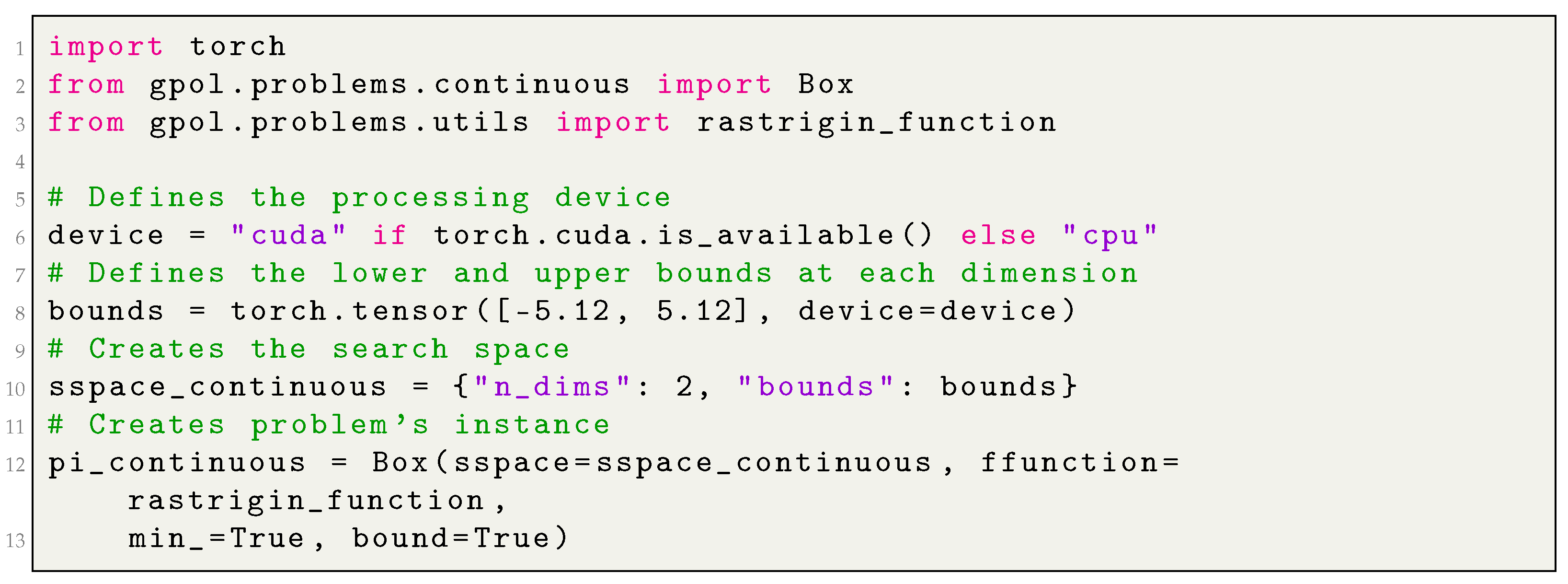
We have conceptualized a module called continuous that contains different problem types from the continuous optimization field. In this release, the module contains one class called Box: a simplistic variant of a constrained continuous problem in which the parameters can take any real number within a given range of values, the box (also known as hyperrectangle), which can be regular case when the bounds are the same for every dimension or irregular when each dimension is allowed to have different bounds. The search space of an instance of the continuous box problem consists of the following key-value pairs.

• “constraints” is a tensor that holds the lower and the upper bounds for the search space’s box. When the box is intended to be regular (i.e., all its dimensions are equally sized), it tensor holds only two values, each representing the lower and the upper bounds of each of the D dimensions of the problem, respectively. When the box is intended to be irregular, the tensor is a 2 ×D matrix. In such case, the first and the second row represent the lower and the upper bounds for each of the D dimensions of the problem, respectively.
• “n_dims” is an integer value representing the dimensionality (D) of S.

When solving hard-constrained continuous problems, some authors in the scientific community bound the solutions to prevent the searching in infeasible regions [19]. The bounding mechanism generally consists of a random re-initialization of the solution on the outlying dimension. For this reason, besides the triplet sspace, ffunction, and min_, an instance of the box problem includes an additional instance-variable called bound, which can optionally activate the solution bounding by assigning it the value True. When bound is set to False, the outlying solution automatically receives the “worst” fitness score (corresponding to the largest or the smallest value allowed by the underlying data type).

Similarly to some popular optimization libraries, such as [6,8], in this release, we implement a wide set of popular continuous optimization test functions (13 in this release): Ackley, Branin, Discus, Griewank, Hyper-ellipsoid, Kotanchek, Mexican Hat, Quartic, Rastrigin, Rosenbrock, Salomon, Sphere, and Weierstrass. The formal definitions and characteristics of the aforementioned functions can be found in [20,21].

Appendix A.1, in the appendix, provides an example of how to create an instance of Box. Note that, in Section B, examples will be presented of how to solve this problem by using different iterative search algorithms contained in the current release of the library.

2.2. Combinatorial Optimization Problems

When solving an instance of a combinatorial optimization problem, one is generally interested in an object from a finite or, possibly, a countable infinite set that satisfies certain conditions or constraints. Such an object can be an integer, a set, a permutation, or a graph [15]. This section introduces two fundamental and popular problems in the combinatorial optimization field that are implemented in the library’s current release: the traveling salesman problem (TSP) and the knapsack problem.

2.2.1. The Traveling Salesman Problem

The TSP is a popular NP-hard combinatorial problem, of high importance in theoretical and applied computer science and operations research. It inspired several other important problems, such as vehicle routing and traveling purchaser [22]. In simple terms, the traveling salesman must visit every city in a given region exactly once and then return to the starting point. The problem proposes the following question: given the cost of travel between all the cities, how should the itinerary be planned to minimize the total cost of the entire tour.

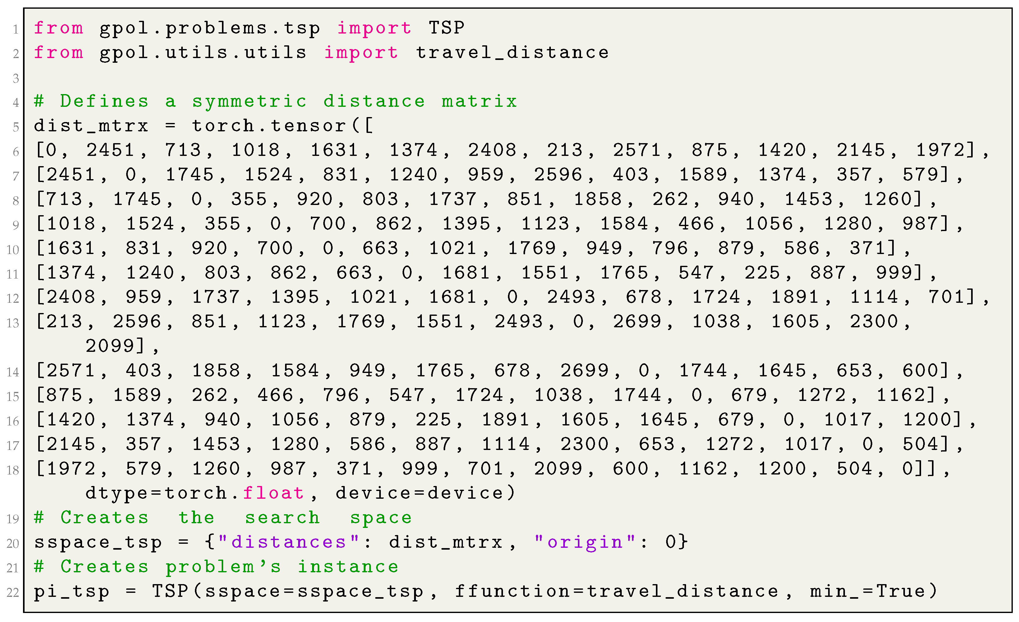
We have conceptualized an eponymous module, designed to contain major variants of the TSP. In this release, the module contains one class called TSP. The search space of an instance of TSP consists of the following key-value pairs:

• “distances” is an $n\times n$ tensor of type torch.float, which represents the distance’s matrix for the underlying problem. The matrix can be either symmetric or asymmetric. A given row i in the matrix represents the set of distances between the “city” i, as being the origin, and the n possible destinations (including i itself).
• “origin” is an integer value representing the origin (i.e., the point from where the “traveling salesman” departs).

Appendix A.2, in the appendix, provides an example of how to create an instance of TSP, whereas Appendix B demonstrates how to solve this problem by using different iterative search algorithms.

2.2.2. Knapsack

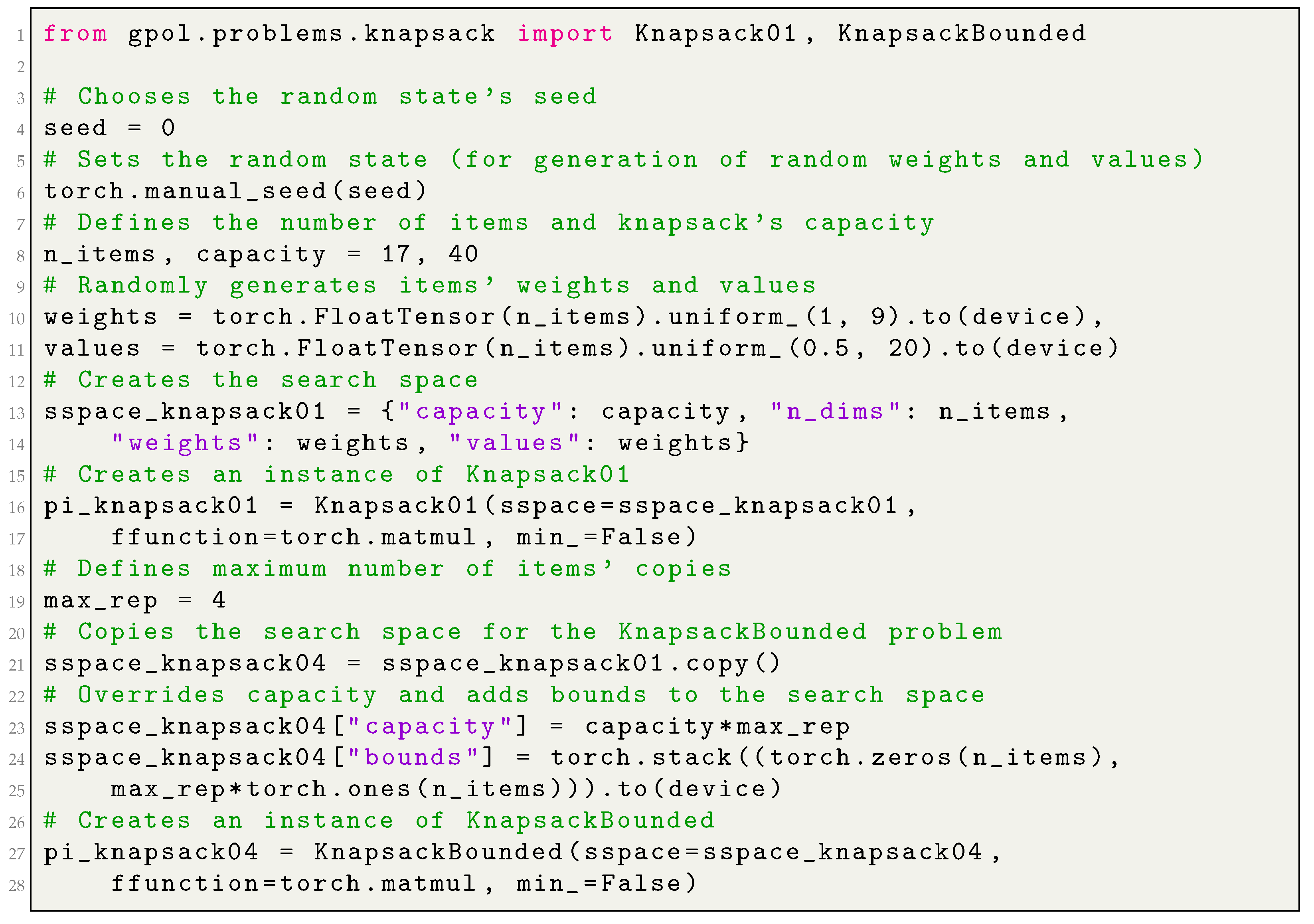
In a knapsack problem, one is given a set of items, each associated with a given value and size (such as the weight and/or volume), and a “knapsack” with a maximum capacity; solving an instance of a knapsack problem implies to “pack” a subset of items into the knapsack, so that the items’ total size does not exceed the knapsack’s capacity, and their total value is maximized. If the total size of the items exceeds the capacity, a solution is considered unfeasible. There is a wide range of knapsack-based problems, many of which are NP-hard, and large instances of such problems can be approached only by using heuristic algorithms [23]. In this release, the library contains two variants: the “0–1” and the “bounded” knapsack problems, implemented in the module knapsack as classes Knapsack01 and KnapsackBounded, respectively. In the first, each item i can be included in the solution only once; as such, the solutions are often represented as binary vectors. In the second, i can be included in the solution $u{b}_i$ times, at most; as such, the solutions are often represented as integer vectors. Concerning the latter, in our implementation, we also allow the user to define not only the upper bound for i ($u{b}_i$), but also the lower bound ($l{b}_i$). That is, we allow the user to specify the minimum and the maximum number of times an item i can be present in a candidate solution. The search space of an instance of Knapsack01 problem, a subclass of Problem, consists of the following key-value pairs:

• “capacity” as the maximum capacity of the “knapsack”;
• “n_dims” as the number of items in S;
• “weights” as the collection of items’ weights defined as a vector of type torch.float;
• “values” as the collection of items’ values defined as a vector of type torch.float.

The search space of an instance of KnapsackBounded problem, a subclass of Knapsack01, also comprises the key “bounds” which holds a $2\times n$ tensor representing the minimum and the maximum number of copies allowed for each of the n items in S.

Appendix A.3, in the appendix, provides an example of how to create an instance of Knapsack01 and KnapsackBounded, whereas Appendix B demonstrates how to solve this problem type.

2.3. Supervised Machine Learning Problems (Approached from the Perspective of Inductive Programming)

Inductive program synthesis (also known as inductive programming) is a subfield in program synthesis that studies program generation from incomplete information, namely, from the examples for the desired input/output behavior of the program [24,25]. Genetic programming (GP) is one of the numerous approaches for the inductive synthesis characterized by performing the search in the space of syntactically correct programs of a given programming language [25].

In the context of supervised machine learning (SML) problem solving, one can define the task of a GP algorithm as the program/function induction from input/output-examples that identifies the mapping $f:S\to \mathbb{R}$ in the best possible way, generally measured through solution’s generalization ability on previously unseen data.

Given the definitions provided above and to support an automatic program’s induction, we conceptualized a module called inductive_programming which in this release implements two different problems. One is called SML, a subclass of Problem, and aims to support the SML problem solving, more specifically the symbolic regression and binary classification, by means of standard GP and its local-search variants. The second, called SMLGS, aims to provide an efficient support for the same tasks addressed instead by means of geometric semantic GP (GSGP), following the implementation proposed in [26]. The major difference between the two is that the latter does not require storing the GP trees in memory, as it relies on memoization techniques.

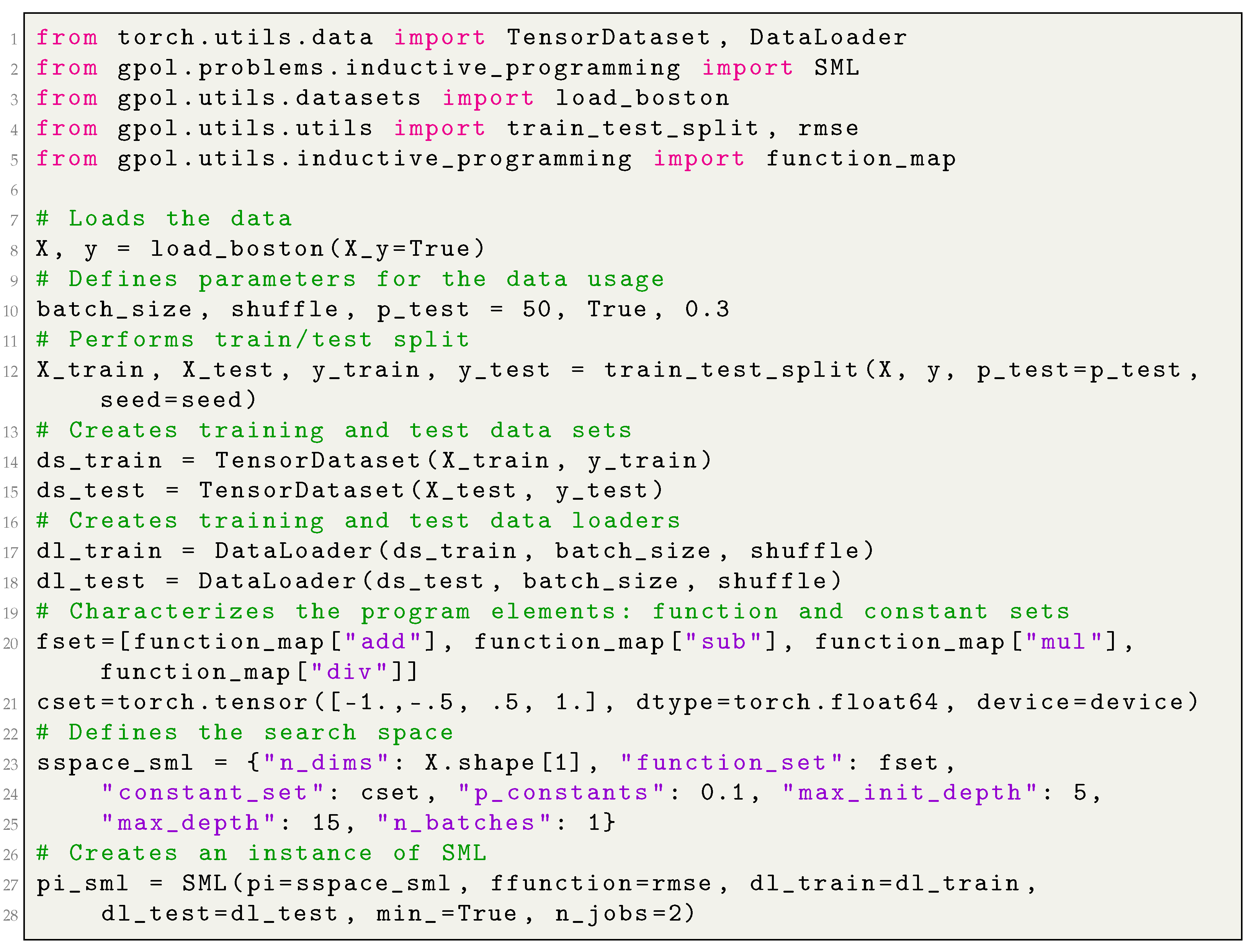
The search space for an instance of SML must contain the problem’s dimensionality (in the context of SML this corresponds to the number of input features), and those GP-specific parameters that characterize and delimit S. These can be the set of functions and constants from which programs are built, the maximum bound for the trees’ initial depth and their growth during the search (which can be seen as a constraint to solutions’ validity), and so forth. The following list of key-value pairs fully describes the search space for an instance of SML:

• “n_dims” is the number of input features (also known as input dimensions) in the underlying SML problem;
• “function_set” is the set of primitive functions;
• “constant_set” is the set of constants to draw terminals from;
• “p_constants” is the probability of generating a constant when sampling a terminal;
• “max_init_depth” is the trees’ maximum depth during the initialization;
• “max_depth” is the trees’ maximum depth during the evolution;
• “n_batches” is number of batches to use when evaluating solutions (more than one can be used).

Besides the traditional triplet sspace, ffunction, and min_ the constructor of SML additionally receives two objects of type torch.utils.data.DataLoader, called dl_train and dl_test, which represent training and test (also known as unseen) data, respectively. In the proposed library, we decided to rely upon PyTorch’s data manipulation facilities, such as torch.utils.data.Dataset and torch.utils.data.DataLoader [27], for the following reasons: simplicity and flexibility of the interface, randomized access of the data by batches, and the framework’s popularity (as such, familiarity with its features). Moreover, the constructor of SML receives another parameter, called n_jobs, which specifies the number of jobs to run in parallel when executing trees (we rely on joblib for parallel computing [28]).

The search space for an instance of SMLGS does not vary from the one of SML except in the fact that it does not take “max_depth” as the growth of the individuals in GSGP is an inevitable and necessary consequence of semantic operators’ application; thus, restricting the depth of the individuals is unnecessary. The constructor of SMLGS is significantly different from the SML in the sense that data are not manipulated through PyTorch’s data-loaders; instead, it uses the input and the target tensors (X and y) directly (similar to what is done in scikit-learn [29]). This difference was motivated by implementation guidelines in [26]. The module gpol.utils.datasets provides a set of built-in regression and classification datasets.

Appendix A.4, in the appendix, provides an example of how to create an instance of SML and SMLGS, whereas Appendix B demonstrates how to solve this problem type.

3. Iterative Search Algorithms

To solve a problem’s instance, one needs to define an optimization algorithm. This library focuses on the iterative search algorithms (also known as metaheuristics), and the current release comprises their stochastic branch.

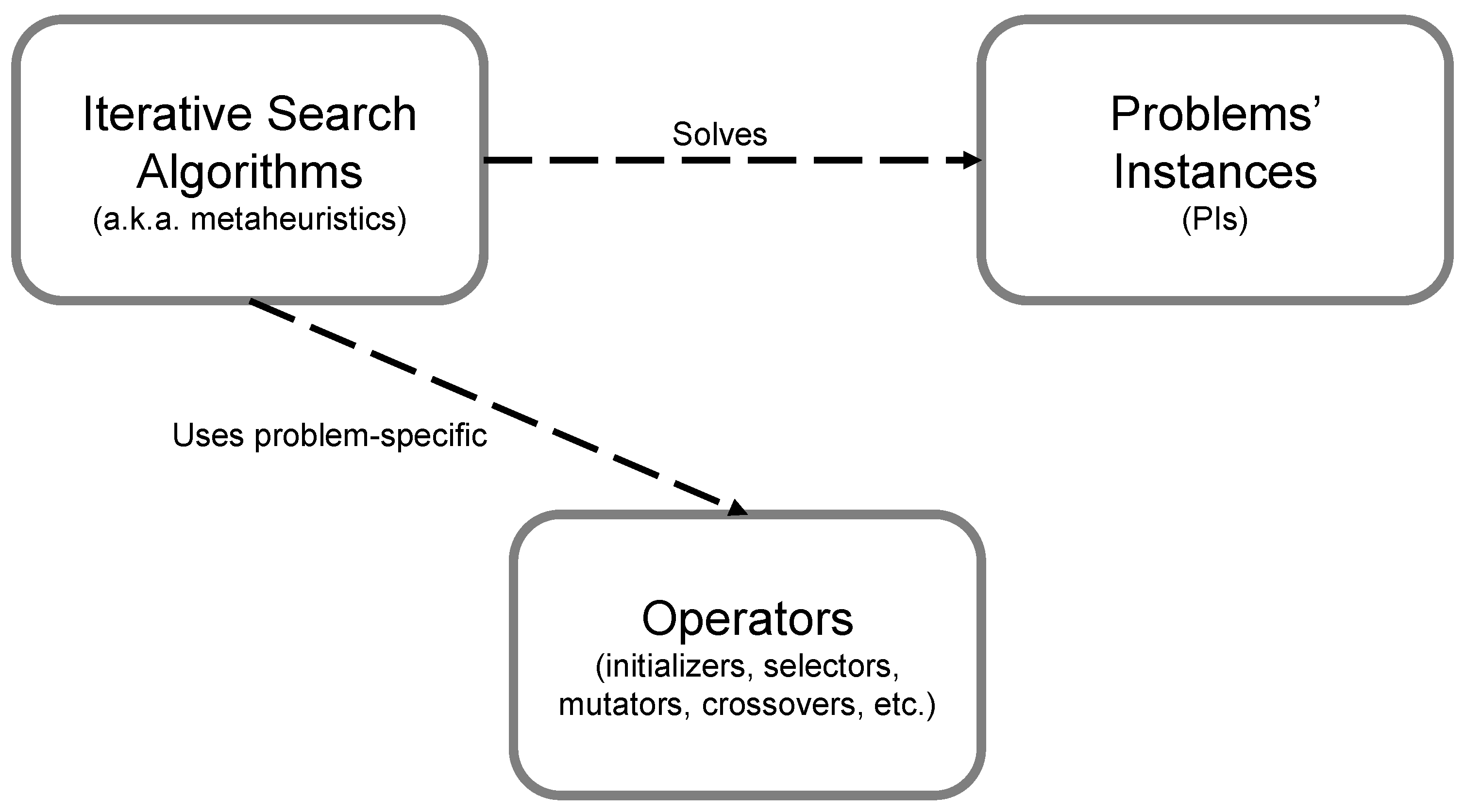
One of the main ideas of the proposed library is to maximally separate the algorithms’ implementation from the problems’ details. The highest manifestation of this aim translates into the possibility to apply a given algorithm for any kind of problem, even if solutions’ generalization ability is a concern. We were able to achieve this characteristic thanks to an abstraction of the metaheuristics from the solutions’ representation and search-related operators, such as initializers, selectors, mutators and crossovers. The block diagram presented in Figure 1 reflects a high-level overview of how the algorithms relate to the problems’ instances and operators.

Based on the number of candidate solutions they handle at each step, the metaheuristics can be categorized into Single-Point (SP) and Population-Based (PB) approaches. The search procedure in the SP metaheuristics is generally guided by the information that is provided by a single candidate solution from S, usually the best-so-far solution, that is gradually evolved in a well-defined manner in hope to find the global optimum. The Hill Climbing and Simulated Annealing, which will be discussed in Section 3.2), are examples of SP metaheuristics. Contrarily, the search procedure in PB metaheuristics is generally guided by the information shared by a set of candidate solutions and the exploitation of the collective behavior in different ways. In abstract terms, one can say that every PB metaheuristics shares, at least, the following two features: an object representing the set of simultaneously exploited solutions (i.e., the population), and a procedure to “move” them across S [30].

In abstract terms, a metaheuristic starts with a point in S and searches, iteration by iteration, for the best possible solution in the set of candidate solutions, according to some criterion. Usually, the stopping criterion is the maximum number of iterations specified by the user [30]. Following this rationale, we have conceptualized an abstract class called SearchAlgorithm, characterized by the following instance attributes:

• pi is an instance of an optimization problem (i.e., what to solve/optimize);
• best_sol is the best solution found by the search procedure;
• initializer is a procedure to generate the initial point in S; and
• device is the specification of the processing device (i.e., whether to perform computations on the CPU or the GPU).

Theoretically, to solve a problem’s instance, the search procedure of an iterative metaheuristic comprises two main steps:

• Initializing the search at a given point in S.
• Solving a problem’s instance by iteratively searching, throughout S, for the best possible solution according to the criteria specified in the instance. Traditionally, the termination condition for an iterative metaheuristic is the maximum number of iterations, and it constitutes the default stopping criterion implemented in this library (although the user can specify a convergence criterion, and the search can be automatically stopped before completing all the iterations).

The two aforementioned steps are materialized as abstract methods _initialize and solve. Every implemented algorithm in the scope of this library is an instance of SearchAlgorithm, meaning that it must implement those two methods. Note that the _initialize is called within the solve, whereas the latter is to be invoked by the main script. The signature for the solve does not vary among different iterative metaheuristics and is made of the following parameters:

• n_iter is the number of iterations to execute a metaheuristic (functions as the default stopping criterion).
• tol is the minimum required fitness improvement for n_iter_tol consecutive iterations to continue the search. When the fitness the current best solution is not improving by at least tol for n_iter_tol consecutive iterations, the search will be automatically interrupted.
• n_iter_tol is the maximum number of iterations to not meet tol improvement.
• start_at is the initial starting point in S (i.e., the user can explicitly provide the metaheuristic a starting point in S).
• test_elite is an indication whether to evaluate the best-so-far solution on the test partition, if such exists. This regard only those problem types which operate upon training and test cases, this allow one to assess solutions’ generalization ability.
• verbose is the verbosity level of the search loop.
• log is the detail level of the log file (if such exists).

Being the root of all the metaheuristics, the SearchAlgorithm class implements the following utility methods:

• _get_best compares two candidate solutions based on their fitness values and returns the best;
• _get_worst compares two candidate solutions based on their fitness values and returns the worst.

Furthermore, the class defines two abstract methods that have to be overridden by the respective subclasses:

• _create_log_event is designed to create a log-event for writing search-related data on the log-file;
• _verbose_reporter is designed to report search-related information on the console.

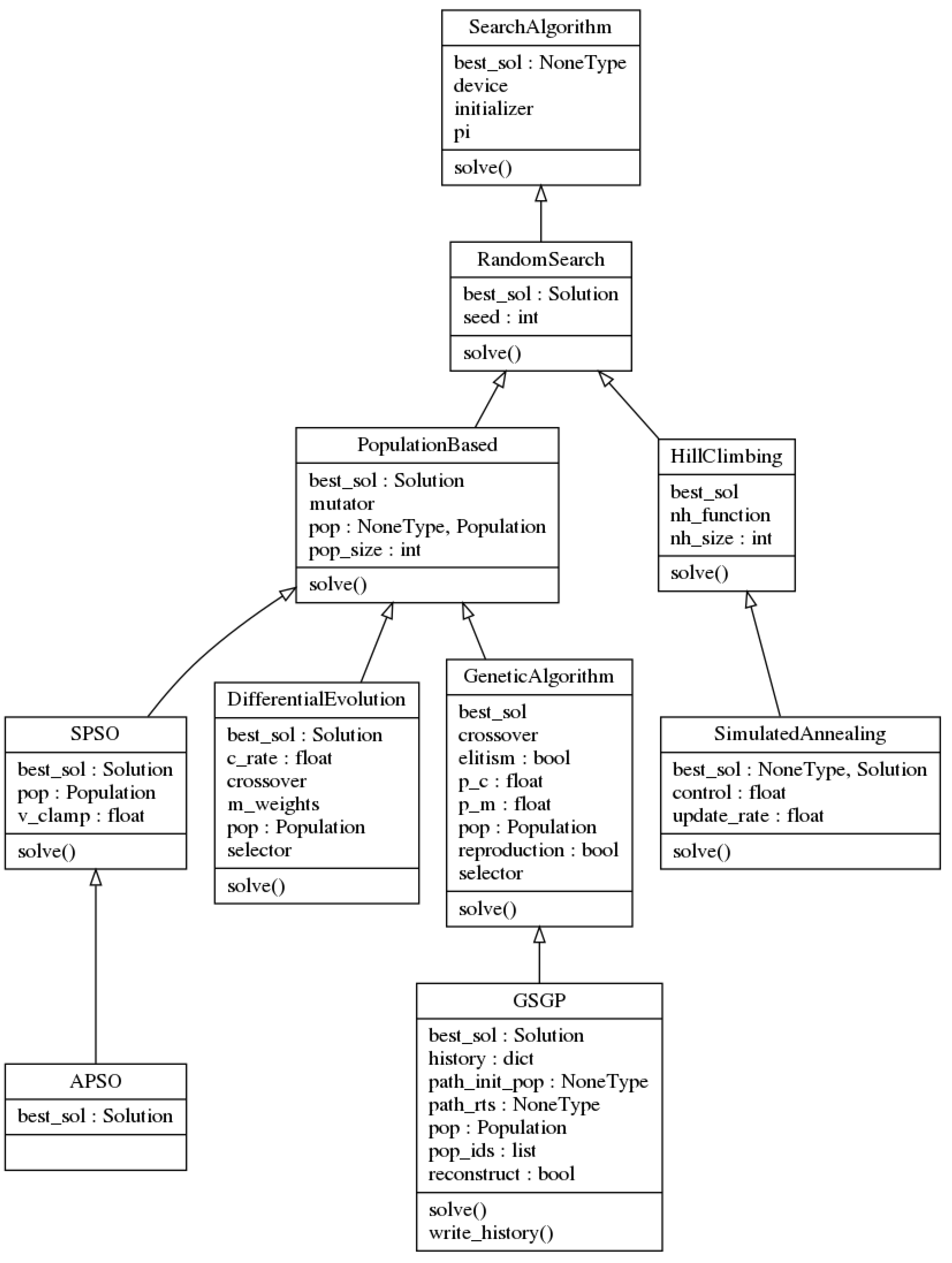
Figure 2 illustrates the UML diagram of the SearchAlgorithm class and its subclasses, which are described in the rest of this section.

3.1. Random Search

The random search (RS) can be seen as the first rudimentary stochastic metaheuristic for problem solving. Its strategy, far away from being “intelligent”, consists of randomly sampling S for a given number of iterations. In the scientific community, RS is frequently used in the benchmarks as the baseline during the algorithms’ performance assessment. Following this rationale, one can conceptualize the RS at the root of the hierarchy of “intelligent” metaheuristics; from this perspective, it is meaningful to assume that metaheuristics donated with “intelligence”, like Simulated Annealing or Genetic Algorithms, might be seen as improvements upon RS, thereby branching from it.

Following this rationale, we have conceptualized a class called RandomSearch, a subclass of SearchAlgorithm, characterized by the following instance attributes:

• pi, best_sol, initializer, and device, which are inherited from the SearchAlgorithm;
• seed which is a random state for the pseudo-random numbers generation (an integer value).

As a subclass of the SearchAlgorithm, the RandomSearch implements the methods _initialize, solve, _create_log_event and _verbose_reporter. Moreover, it implements _get_random_sol, a method that (1) generates a random representation of a candidate solution by means of the initializer, (2) creates an instance of type Solution, (3) evaluates an instance’s representation, and (4) returns the evaluated object.

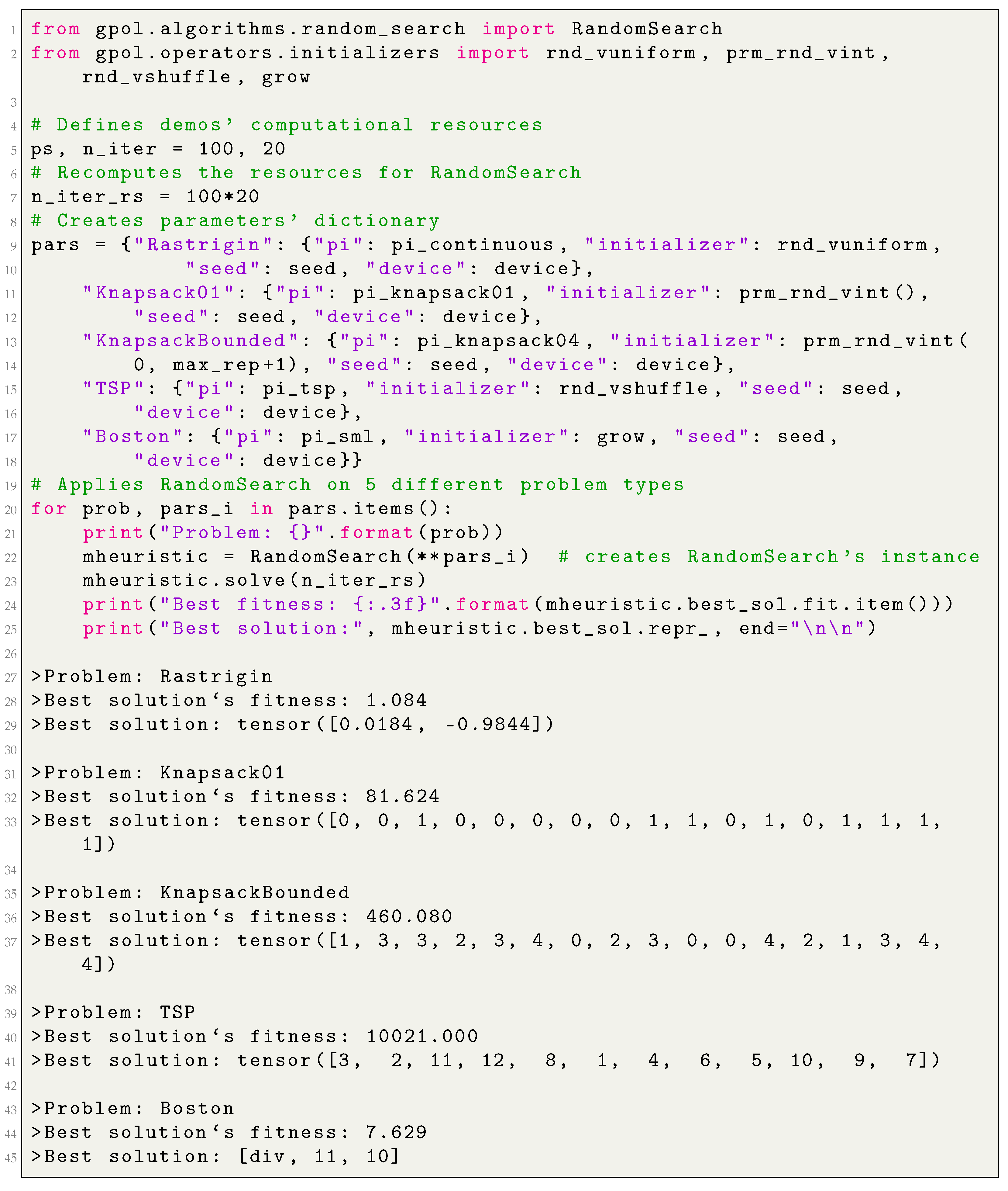
Appendix B.1 demonstrates how to create an instance of RandomSearch and apply it in different problem solving.

3.2. Local Search

The local search (LS) algorithms can be seen among the first intelligent search strategies that improve the functioning of the RS. They rely upon the concept of neighborhood which is explored at each iteration by sampling from S a limited number of neighbors of the best-so-far solution. Usually, the LS algorithms are divided in two branches. In the first branch, called hill climbing (HC), or hill descent for the minimization problems, the best-so-far solution is replaced by its neighbor when the latter is at least as good as the former. The second branch, called simulated annealing (SA), extends HC by formulating a non-negative probability of replacing the best-so-far solution by its neighbor when the latter is worse. Traditionally, such a probability is small and time-decreasing. The strategy adopted by SA is especially useful when the search is prematurely stagnated at a locally sub-optimal point in S.

Given the definitions provided above, we have conceptualized a module called local_search, which contains different LS meta-heuristics. In this release, we implement the HC and SA algorithms. The former is materialized as a subclass of the RandomSearch, called HillClimbing, whereas the latter is materialized as a subclass of HillClimbing, called SimulatedAnnealing.

To solve a given problem’s instance, a LS algorithm mainly requires problem-specific initialization and neighborhood functions. For example, the candidate solutions for the 0-1 Knapsack problem are, technically, fixed length vectors of Boolean values; as such, a neighbor should also be an equal vector of the same data type, whose values are in a “neighboring” arrangement. Given that the initialization, and in the case of LS, the neighbors’ generation functions are provided at the moment of algorithms’ instantiating, one can create an instance of RandomSearch, HillClimbing, or SimulatedAnnealing to solve potentially any kind of problem, whether it is continuous, combinatorial, or inductive program synthesis for SLM problem solving. The only two things one has to take in consideration are the correct specification of the search space and the operators for a given problem type.

3.2.1. Hill Climbing (HC)

HC is a popular meta-heuristics in the field of optimization which has been successfully applied in several domains, including continuous and combinatorial optimization [31]. Moreover, there is evidence of the successful adaptation of HC in the context of inductive-programming synthesis for neuroevolution [32]. In general terms, HC searches for the best possible solutions by iteratively sampling a set of neighbors of the current best solution, using the neighborhood function, and choosing the one with the best fitness. Within this library, the HC algorithm is materialized through the class HillClimbing, subclass of RandomSearch and it is characterized by the following instance attributes:

• pi, initializer, best_sol, seed, and device are the instance attributes inherited from RandomSearch;
• nh_size is the neighborhood’s size;
• nh_function is a procedure to generate nh_size neighbours of a given solution (the neighbour-generation function).

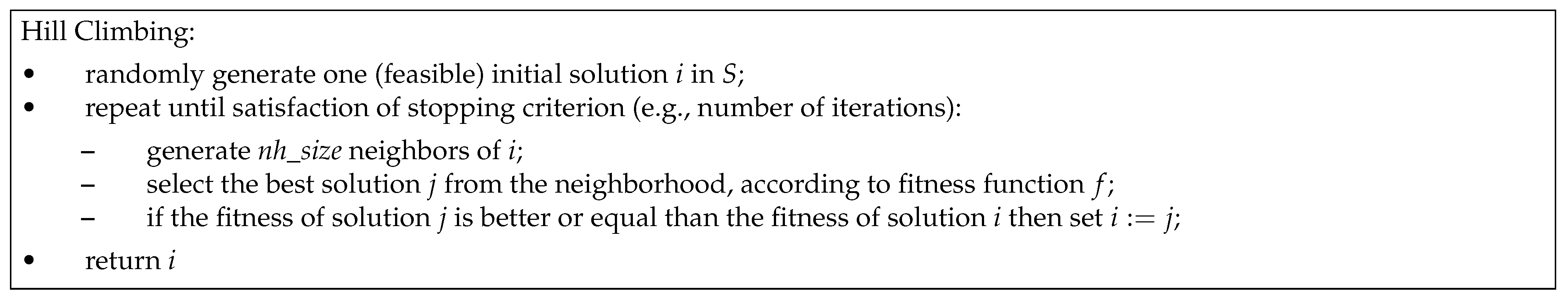
The main distinctive characteristics of the HillClimbing class can be expressed through the logic that guides the search-procedure, which is implemented in the overridden solve method. Additionally, the class implements a private method, called _get_best_nh, which returns the best neighbor from a given neighborhood. Figure 3 represents the search procedure of a HC algorithm that is mirrored in the solve method.

3.2.2. Simulated Annealing (SA)

The HC algorithm suffers from several limitations, namely, it frequently becomes stuck at the local optima. To overcome this problem, the scientific community proposed several approaches, among them the SA algorithm that also uses the notion of the neighborhood [14]. One thing that distinguishes SA from HC is an explicit ability to escape from the local optima. This ability was conceived by simulating, in the computer, a well-known phenomenon in metallurgy called annealing (which is why the algorithm is called simulated annealing). Following what happens in metallurgy, in SA, the transition from the current state (the best-so-far candidate solution i), to a candidate new state (a neighbor of i), can happen for two reasons: either because the candidate state is better, or following the outcome of an acceptance probability function—a function that probabilistically accepts a transition toward the new candidate state, even if it is worse than the current state, depending on the the states’ energy (fitness) and a global (time-decreasing) parameter called the temperature (t) [14]. From this perspective, SA can be seen as an attempt to improve upon HC by adding more “intelligence” in the search strategy. Within this library, the SA algorithm is materialized through the class SimulatedAnnealing, subclass of HillClimbing, and it is characterized by the following instance attributes:

• pi, initializer, nh_function, nh_size, best_sol, seed, and device are instance attributes inherited from HillClimbing;
• control is the control parameter (also known as temperature);
• update_rate: rate of control’s decrease over the iterations.

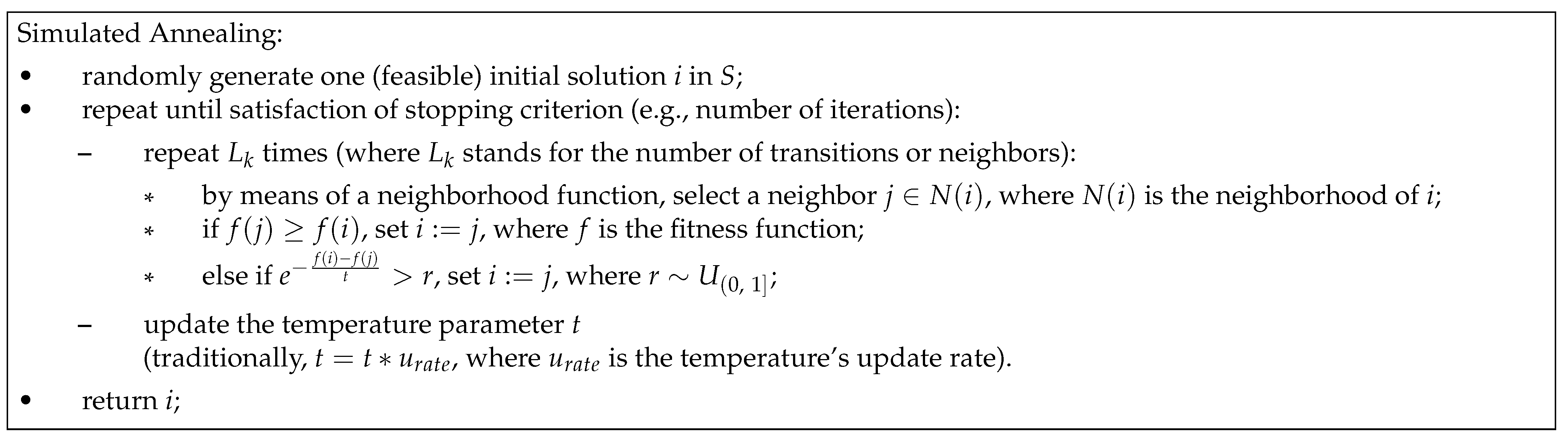
The Figure 4 provides the main steps of SA (for a maximization problem), that are mirrored in the solve method of SimulatedAnnealing class.

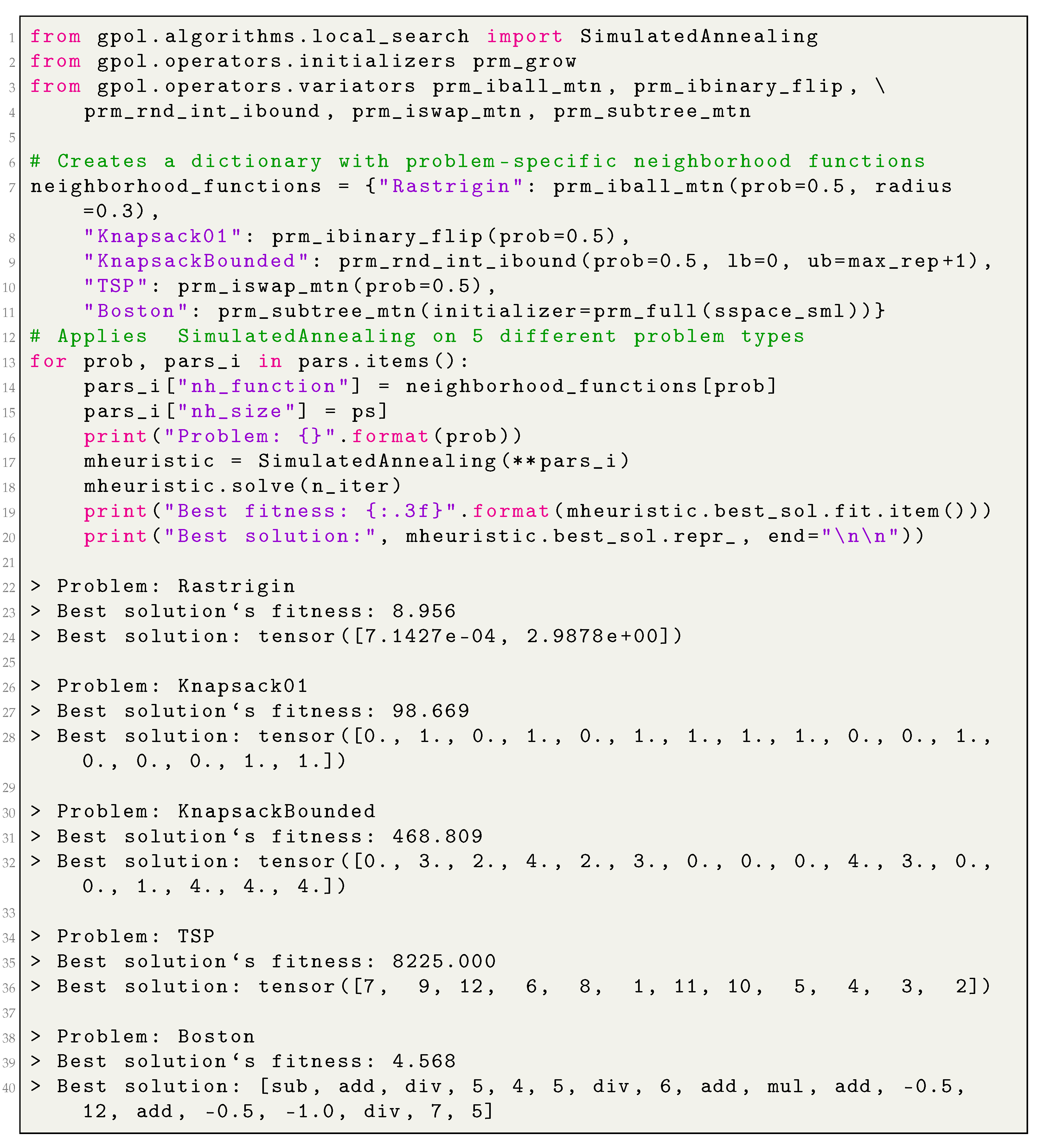
Appendix B.2 demonstrates how to create an instance of SimulatedAnnealing and apply it in different problem solving.

3.3. Population-Based Algorithms

Given the fact we are aiming at a library focused on SP and PB metaheuristics, we have conceptualized an abstract class called PopulationBased, a subclass of RandomSearch, as it improves the latter by means of “collective intelligence.” The class PopulationBased is the root of all the PB-metaheuristics and is characterized by the following instance attributes:

• pi, initializer, best_sol, seed, and device are inherited from the RandomSearch;
• pop_size is the number of candidate solutions to exploit simultaneously at each step (i.e., the population’s size);
• pop is an object of typePopulation representing the set of simultaneously exploited candidate solutions (i.e., the population);
• mutator is a procedure to “move” the candidate solutions across S.

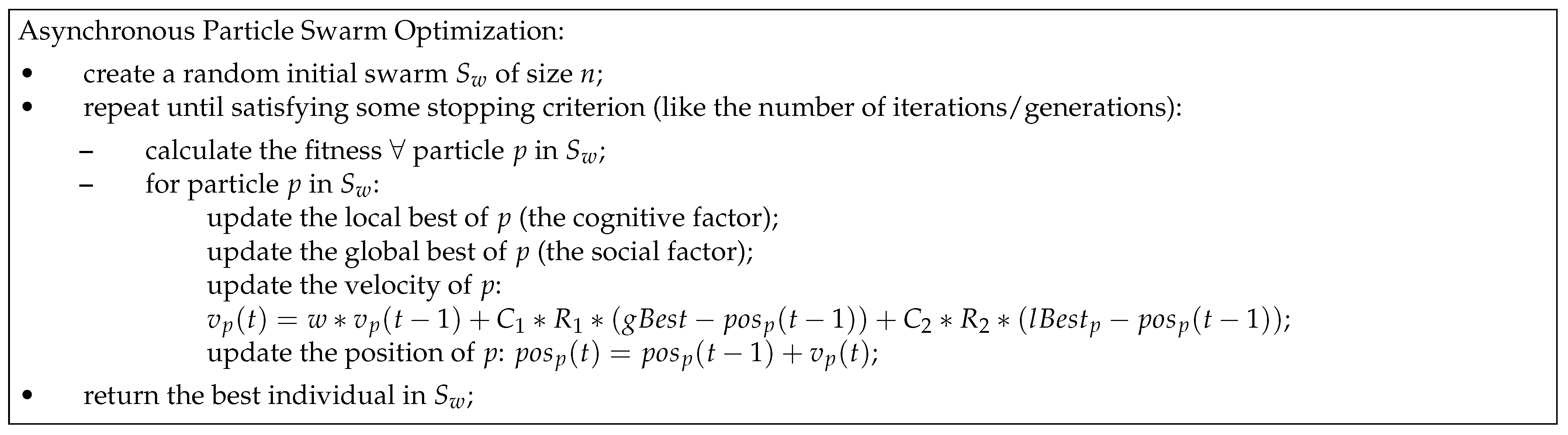
The current release of GPOL presents five PB metaheuristics: genetic algorithm (GA), genetic programming (GP), geometric semantic genetic programming (GSGP), differential evolution (DE) and particle swarm optimization (PSO). The latter is present in two variants that differ in the precedence candidate solutions (called particles) update their positions: synchronous-PSO (SPSO) and asynchronous-PSO (APSO). The objective of the following sections is to describe these algorithms and show how they can be used to solve different problems.

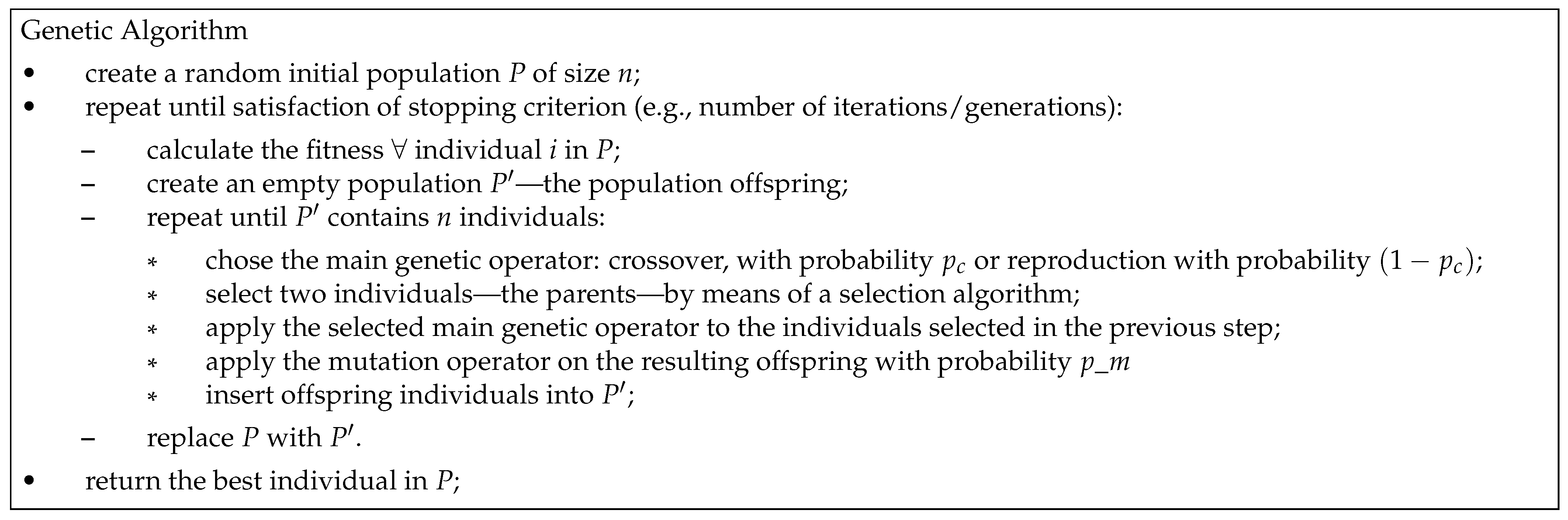
3.3.1. Genetic Algorithms (GAs)

Genetic algorithms (GAs) is a metaheuristic introduced by J. Holland [33], which was strongly inspired by Darwin’s theory of evolution by means of natural selection [34]. Conceptually, the algorithm starts with a random-like population of candidate solutions (called chromosomes). Then, by mimicking the natural selection and genetically-inspired variation operators, such as the crossover and the mutation, the algorithm breeds a population of the next-generation candidate solutions (called the offspring population, $P^{\prime }$), which replaces the previous population (also known as the parent population, P). This procedure is iterated until reaching some stopping criteria, such as a maximum number of iterations (also called generations) [35].

Following the above-presented rationale, we have conceptualized a class called GeneticAlgorithm, subclass of PopulationBased, characterized by the following instance attributes:

• pi, initializer, best_sol, pop_size, pop, mutator, seed, and device are inherited from PopulationBased;
• selector is the selection operator;
• crossover is the crossover variation operator;
• p_m is the probability of applying mutation variation operator;
• p_c is the probability of applying crossover variation operator;
• elitism is a flag which activates elitism during the evolutionary process; and
• reproduction is a flag that states whether the crossover and the mutation can be applied on the same individual (case when reproduction is set to True). If reproduction is set to False, then either crossover or mutation will be applied (this resembles a GP-like search procedure).

Figure 5 presents the main steps of the solve method in the GeneticAlgorithm class. Moreover, the class implements a private method, called _elite_replacement, which directly replaces P with $P^{\prime }$ if the elite is the best offspring; otherwise, when the elite is the best parent, P is replaced with $P^{\prime }$ and the elite is transferred to $P^{\prime }$ (by replacing a randomly selected offspring).

3.3.2. Genetic Programming (GP)

Genetic programming (GP) is a PB metaheuristic, proposed and popularized by J. Koza [36], which extends GAs to allow the exploration of the space of computer programs. Similarly to other evolutionary algorithms (EAs), GP evolves a set of candidate solutions (the population) by mimicking the basic principles of Darwinian evolution. The evolutionary process involves fitness-based selection of the candidate solutions and their variation by means of genetically-inspired operators (such as the crossover and the mutation) [36,37]. If abstracted from some implementation details, GP can be seen as GA, in which initialization and variation operators were specifically adjusted to work upon tree-based representations of the solutions (this idea was inspired by the LISP programming language, in which programs and data structures are represented as trees). Concretely, programs are defined using two sets: a set of primitive functions, which appear as the internal nodes of the trees, and a set of terminals, which represent the leaves of the trees. In the context of SML problem solving, the trees represent mathematical expressions in the so-called Polish prefix notation, in which the operators (primitive functions) precede their operands (terminals). Given that the initialization, selection, and variation operators are provided as constructor’s parameters, one can create an instance of GeneticAlgorithm to solve potentially any kind of problem, whether it is of continuous, combinatorial, or inductive program synthesis nature. The only two things one has to take into consideration are (1) the correct specification of the problem-specific S and (2) the operators. Following this perspective, by creating an instance of the class GeneticAlgorithm with, for example, ramped half-and-half (RHH) initialization, tournament selection, swap crossover and sub-tree mutation, all of them implemented in this library, one obtains a standard GP algorithm. Recall that a similar flexible behaviour is present in the branch of LS algorithms. By providing HC or SA with, for example, grow initialization and sub-tree mutation, one obtains a LS-based program induction algorithm.

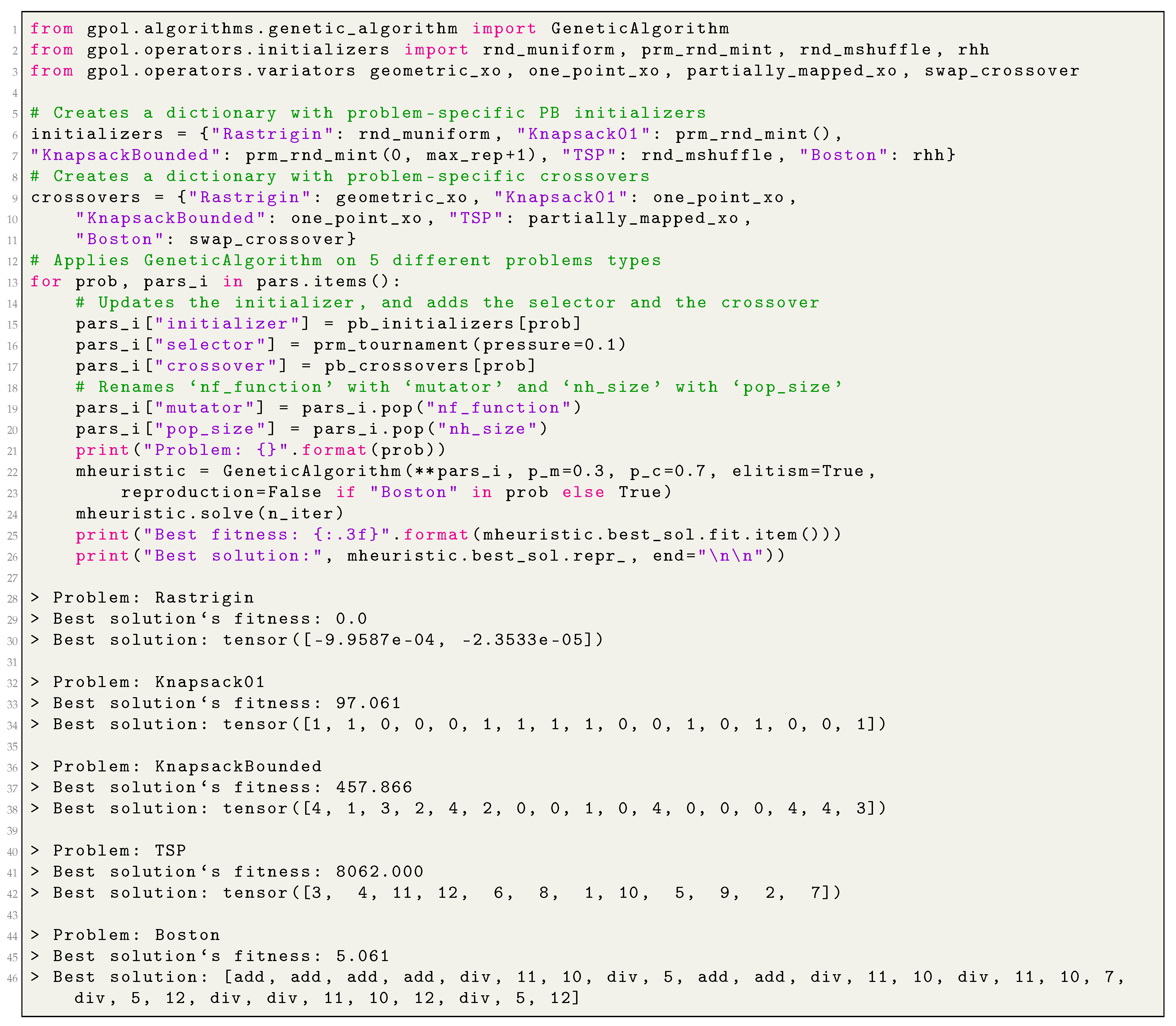
Appendix B.3 demonstrates how to create an instance of GeneticAlgorithm and apply it in different problem solving.

3.3.3. Geometric Semantic Genetic Programming (GSGP)

Geometric semantic genetic programming (GSGP) is a variant of GP in which the so-called geometric semantic operators (GSOs) replace the standard crossover and mutation operators [38].

GSOs gained popularity in the GP community [39,40,41,42,43] because of their geometric property of inducing a unimodal error surface (characterized by the absence of locally optimal solutions) for any SML problem, which quantifies the quality of candidate solutions by means of a distance metric between the target and their output values (also known as semantics). The formal proof of this property can be found in [38,44].

A geometric semantic crossover (GSC) generates, as the unique offspring of parents $T_1,T_2:{\mathbb{R}}^n\to \mathbb{R}$, the expression: $T_{XO}=(T_1·T_R)+((1-T_R)·T_2)$, where $T_R$ is a random real function whose output values range in the interval $[0,1]$. Moraglio and coauthors [38] show that GSC corresponds to geometric crossover in the semantic space (i.e., the point representing the offspring stands on the segment joining the points representing the parents). Consequently, the GSC inherits the key property of geometric crossover: the offspring is never worse than the worst of the parents.

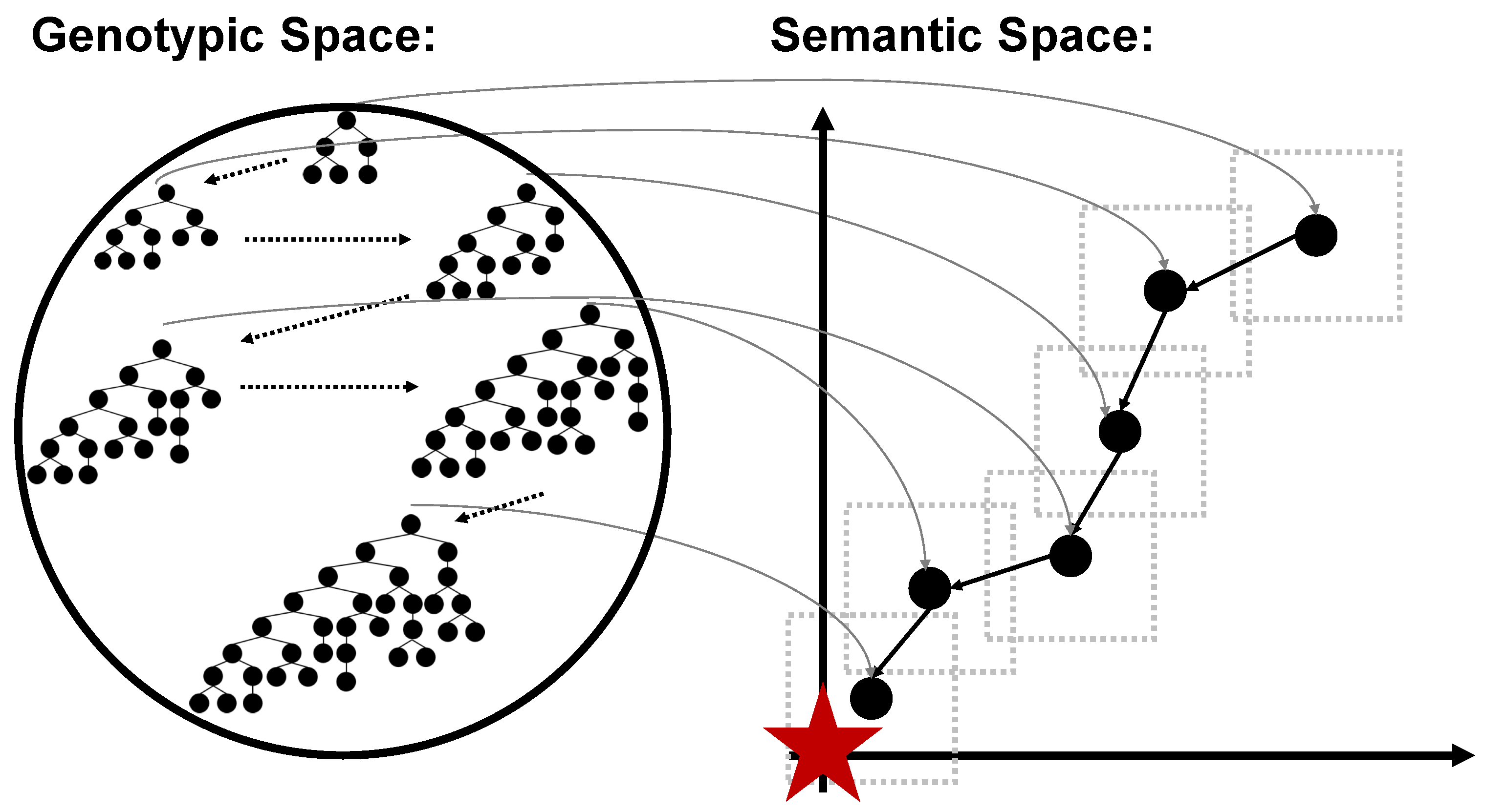
A geometric semantic mutation (GSM) returns, as the result of the mutation of an individual $T:{\mathbb{R}}^n\to \mathbb{R}$, the expression: $T_M=T+ms·(T_{R1}-T_{R2})$, where $T_{R1}$ and $T_{R2}$ are random real functions with a codomain in $[0,1]$ and $ms$ is a parameter called the mutation step. Similarly to GSC, Moraglio and coauthors show that GSM corresponds to a box mutation on the semantic space. Consequently, the operator induces a unimodal error surface on any SML problem.

The demonstration of how GSM induces a unimodal error surface can be found in Figure 6, which represents a chain of possible individuals that could be generated by applying GSM several times and their corresponding semantics (left and right subfigures, respectively). Here, for the sake of visualization, we present a simple 2D semantic space, where each solution is represented by a point (this corresponds to the case when there are only two training instances). The known global is represented with a red star. Each point in the figure is “surrounded” by a gray dotted square of side $ms$, which corresponds to the mutation’s step inside which the GSM allows solutions to move. As one can see, GSM’s application allows for moving a given solution in any position inside the square, including the one that approximates it to the target. Thus, GSM implies that there is always a possibility of getting closer to the target. This implies that no local optima, except the global optimum, can exist, and the fitness landscape for this problem is unimodal. The gray arrows map the genotypic space to the phenotypic and highlight GSM’s capability of generating a transformation on the trees’ syntax, which has an expected effect on their semantics [44].

However, as Moraglio et al. [38] noted, GSOs create offspring that are substantially larger than their parents are. Moreover, the fast growth of the individuals’ size rapidly turns the fitness evaluation to slow, making the system unusable. As a solution to this problem, Castelli et al. [45] proposed a computationally efficient implementation of GSOs, making them usable in practice.

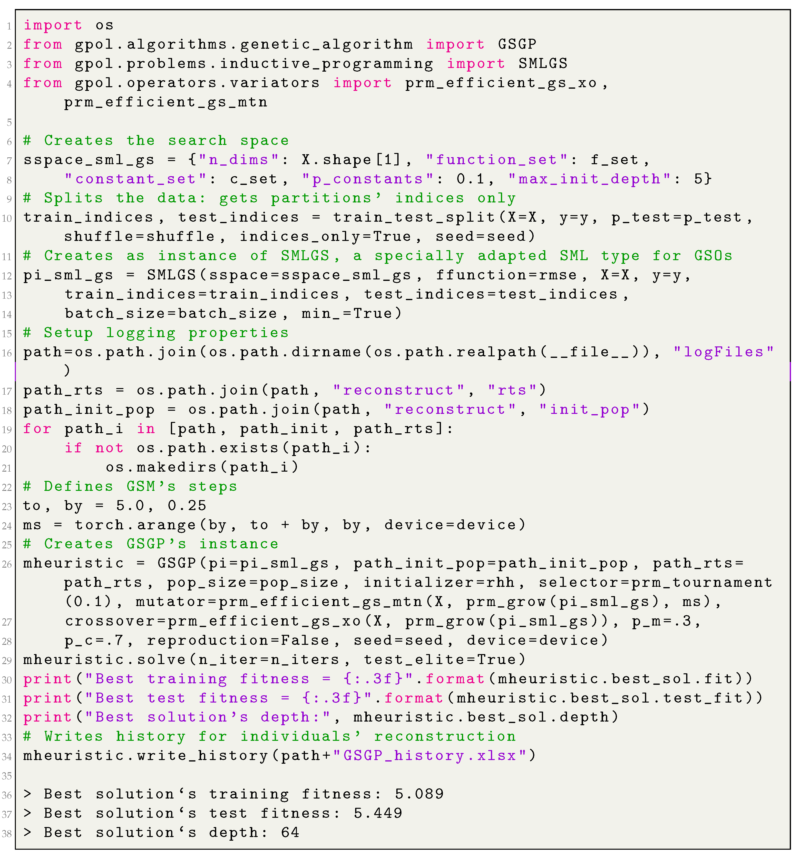
Given the growing importance of GSOs, we decided to include them in our library, following the efficient implementation guidelines proposed in [26]. More specifically, we implemented GSGP through a specialized class called GSGP, a subclass of GeneticAlgorithm, which encapsulates the aforementioned efficient implementation of GSOs and is intended to work in conjunction with SMLGS (which was also specially designed to incorporate the aforementioned guidelines). The class GSGP is characterized by the following instance attributes:

• pi, best_sol, pop_size, pop, initializer, selector, mutator, crossover, p_m p_c, elitism, reproduction, seed, and device are inherited from the GeneticAlgorithm class.
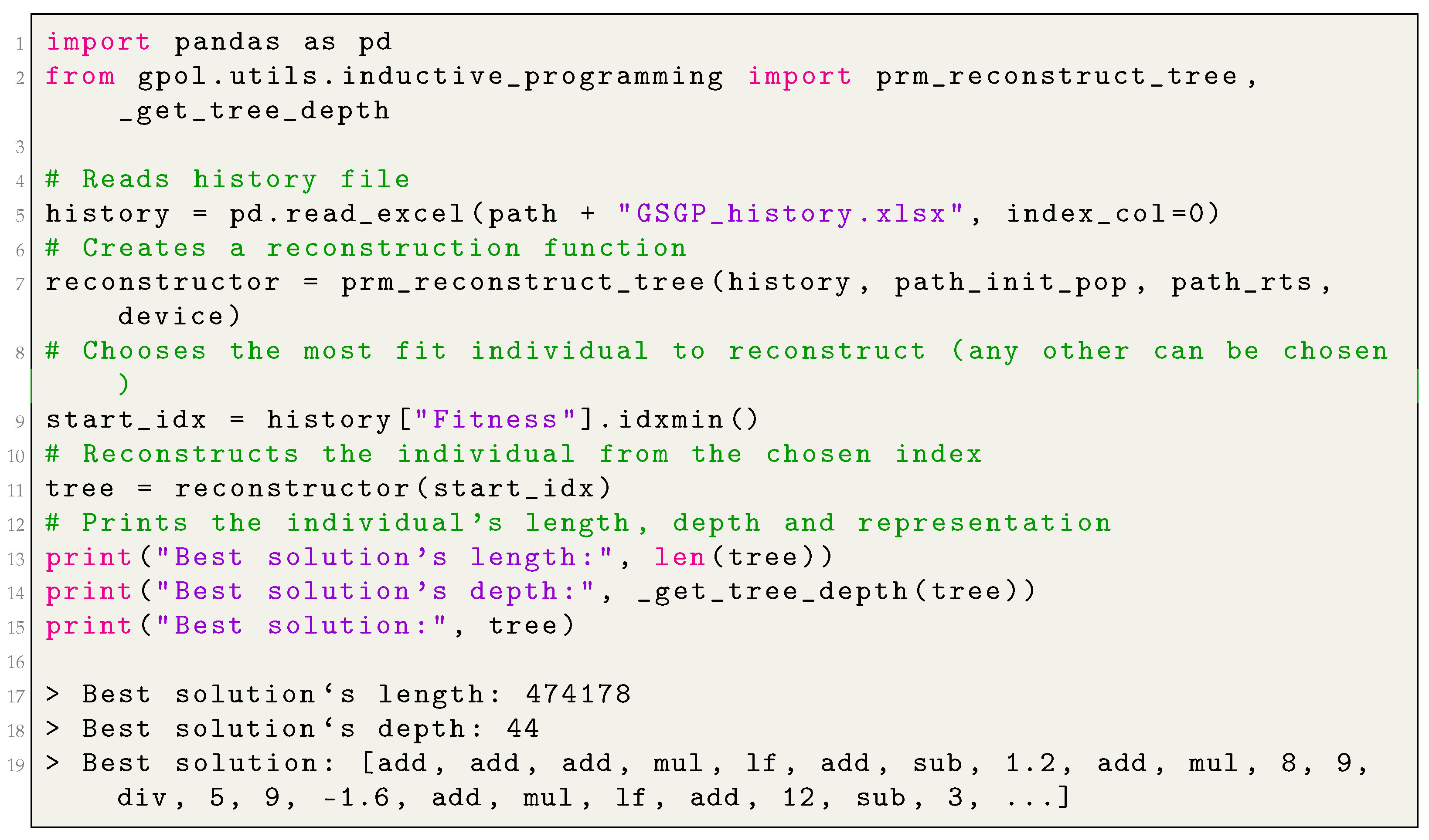
• _reconstruct is a flag stating whether the initial population and the intermediary random trees should be disk-cached. If the value is set to “False”, then there is no possibility of reconstructing the individuals after the search is finished; this scenario is useful to conduct the parameter tuning, for example. If the value is set to “True”, then the individuals can be reconstructed by means of an auxiliary procedure (the function gpol.utils.inductive_programming.prm_reconstruct_tree) after the search is finished; this scenario is useful when the final solution needs to be deployed, for example.
• path_init_pop is a connection string toward the initial population’s repository.
• path_rts is a connection string toward the random trees’ repository.
• pop_ids are the IDs of the current population (the population of parents).
• history is a dictionary which stores the history of operations applied on each offspring. In abstract terms, it stores a one-level family tree of a given offspring. Specifically, history stores as a key the offspring’s ID, as a value a dictionary with the following key-value pairs:
  • “Iter” is the iteration’s number; “Operator” is the variation operator that was applied on a given offspring;
  • “T1” is the ID of the first parent;
  • “T2” is the ID of the second parent (if GSC was applied);
  • “Tr” is the ID of a random tree;
  • “ms” is mutation’s step (if GSM was applied);
  • “Fitness” is the offspring’s training fitness.

Moreover, it implements a method called write_history, which writes locally (following a user-specified path) the history dictionary as a table in a comma-separated value (csv) format. This file will feed the aforementioned reconstruction algorithm.

Appendix B.4 demonstrates how to create an instance of GSGP and apply it in different problem solving, whereas Appendix B.5 demonstrates how to reconstruct an individual generated by means of GSGP.

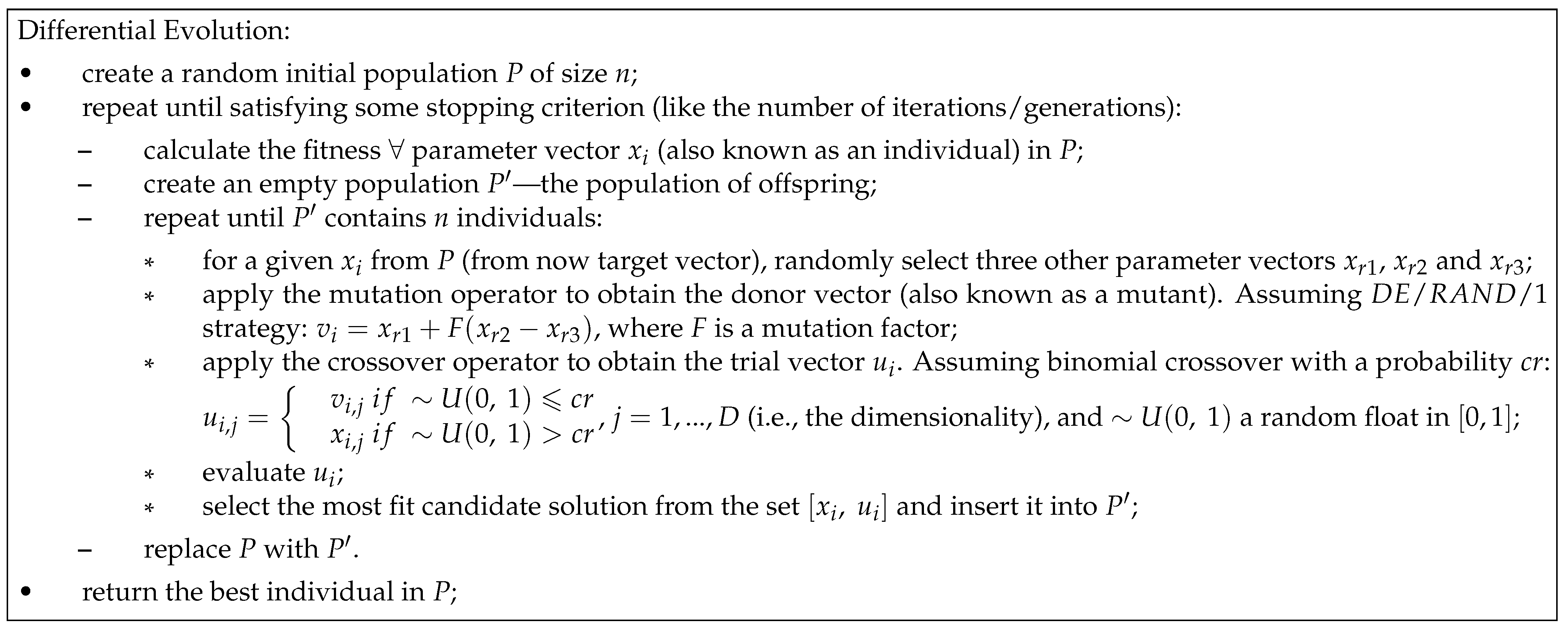
3.3.4. Differential Evolution (DE)

Differential evolution (DE) is another type of metaheuristic that we have considered including in our library. Storn and Price in 1995 [46,47] originally designed this PB metaheuristic for solving continuous optimization problems in 1995. The algorithm shares many similar features with GA, as it involves maintaining a population of candidate solutions, which are exposed to iterative selection and variation (also known as recombination). Nevertheless, DE differs substantially from GA in how the selection and the variation are performed. The parent selection is performed at random, meaning that all the chromosomes have an equal probability of being selected for mating, regardless of their fitness. The variation consists of two steps: mutation and crossover. Numerous different operators were proposed so far [48,49]; however, in this release, we have considered including their original versions [46]. For each parent member (called the target vector), the mutation creates a mutant based on the scaled difference between two randomly selected parents, added to a third (random) population member. The scaling factor F, which controls the amplification of the differential variation, usually lies in $[0.4,1]$ as reported in [50]. In binomial crossover, the type of crossover we have included in the library, the elements of the resulting mutant (called the donor) are exchanged, with probability $C_r$, with the elements of one of the previously selected parents (called the target). That is, the crossover is performed on each of the D indexes of the donor with a probability $C_r$ by exchanging its values with the target vector. The resulting vector, frequently called the trial vector, is then compared with the respective target and the best solution passes to the next iteration.

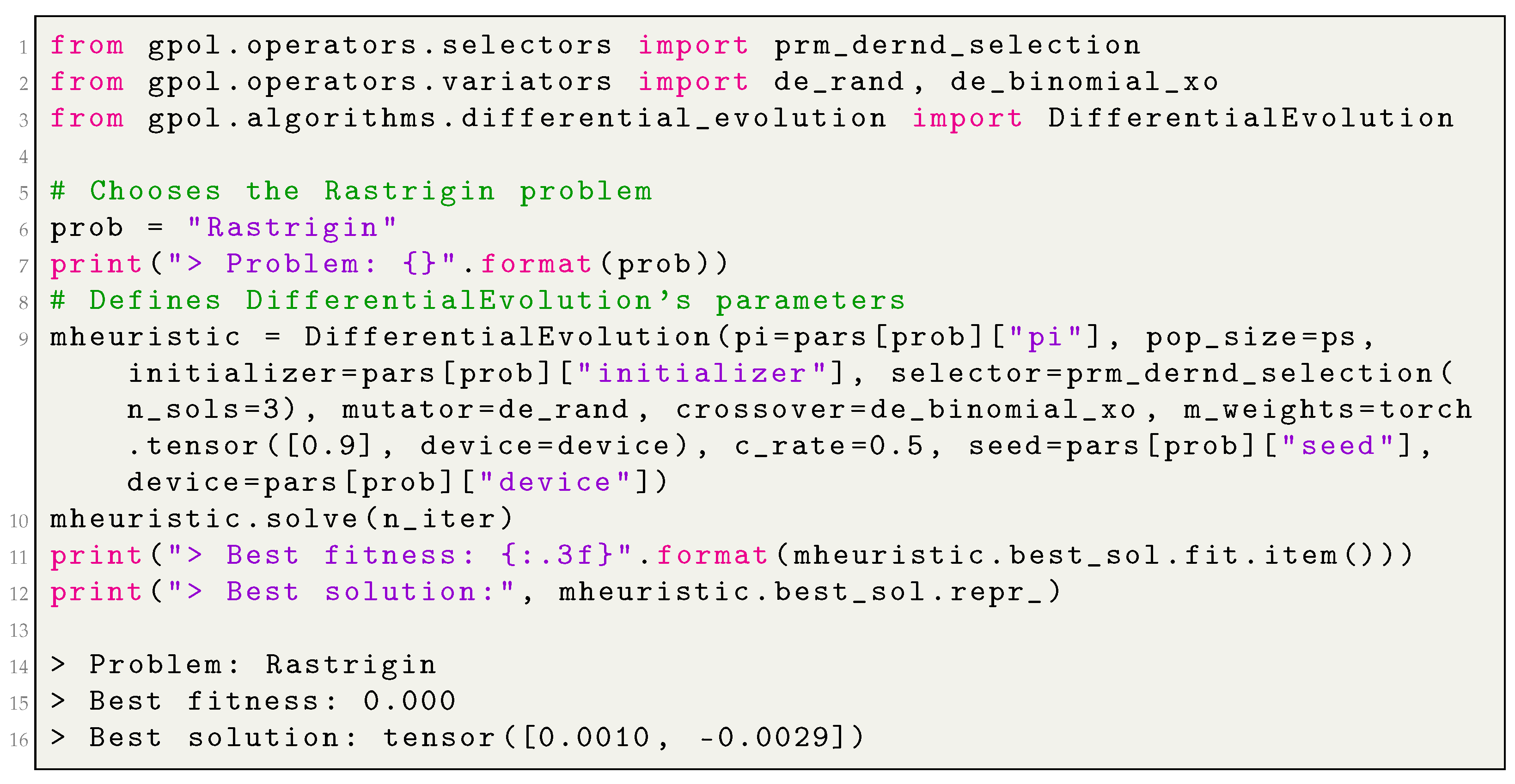
Following the above-presented rationale, we have conceptualized a class called DifferentialEvolution, a subclass of PopulationBased, characterized by the following instance attributes:

• pi, initializer, best_sol, pop_size, pop, mutator, seed, and device are inherited from the PopulationBased;
• selector is an operator that selects parents for the sake of mutation;
• crossover: crossover operator.

At this point, it becomes necessary to clarify some aspects of the nomenclature. Although, in the scope of the original nomenclature, selection stands for the procedure that decides whether trial vectors should become members of the next generation, in this library, selection represents the process of selecting parents for the sake of mutation. This process can be conducted at random, as in the original definition of DE, or can be a function of a solution’s fitness. The selection, as understood by the DE, is implemented in a private method called _replacement: it compares each trial vector with its respective target and returns the most fit solution.

Figure 7 presents the main steps that the solve method of DifferentialEvolution class implements.

It is worth highlighting the high flexibility of the implementation: because of the parents’ selection operator, the mutation and crossover functions are provided as parameters of DifferentialEvolution, and one can easily personalize this PB metaheuristic.

Appendix B.6 demonstrates how to create an instance of DifferentialEvolution and apply it in different problem solving.

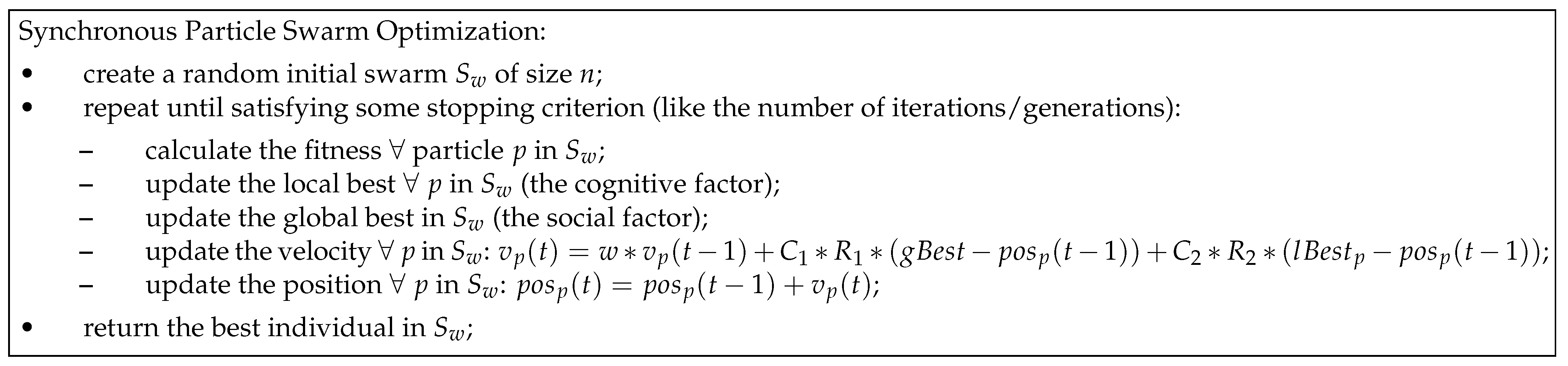
3.3.5. Particle Swarm Optimization

Particle swarm optimization (PSO) is another form of PB metaheuristic, developed by Eberhart and Kennedy in 1995 [51]. Contrarily to previously presented EAs, PSO was inspired by the social behavior of living organisms, such as birds and fish, when looking for food sources. Following PSO’s nomenclature, a population is called swarm, and a candidate solution is a particle.

In PSO, the position of particle p at iteration i, formally represented as ${\overrightarrow{x}}_{p,i}$, is updated at each iteration based on a procedure that takes into account two components: particle’s and swarm’s best-so-far positions. The former (also known as the local best) relates to the cognitive component of the particle (i.e., its memory). The latter (also known as the global best) relates to the social component of the particle (i.e., its cooperation with surrounding neighbors). Since the introduction of PSO, the scientific community has proposed numerous variations to improve its effectiveness. In our library, we rely on the variant of gbest PSO proposed by Shi and Eberhart in 1998 [52], where authors have introduced a new parameter, called inertia weight (w). Formally, the procedure for a particle’s position update is defined as ${\overrightarrow{x}}_{(p,i)}={\overrightarrow{x}}_{(p,i-1)}+{\overrightarrow{v}}_{(p,i)}$, such that ${\overrightarrow{v}}_{(p,i)}=w\ast {\overrightarrow{v}}_{(p,i-1)}+C_1\overrightarrow{{\varphi }_1}({\overrightarrow{lbest}}_p-{\overrightarrow{x}}_{(p,i-1)})+C_2\overrightarrow{{\varphi }_2}(\overrightarrow{gbest}-{\overrightarrow{x}}_{(p,i-1)})$, where ${\overrightarrow{lbest}}_p$ and $\overrightarrow{gbest}$ represent the local and global best, respectively, with $C_1$ and $C_2$ being two positive constants used to scale their contributions in the equation (also known as acceleration coefficients). The quantities $\overrightarrow{{\varphi }_1}$ and $\overrightarrow{{\varphi }_2}$ are two random vectors whose values follow ∼$U(0,1)$ at each dimension. Since a large value of w can help to find a good area through exploration in the beginning of the search, and a small w in the end, when typically a good area was found already, a time-decreasing w can be used instead of a fixed one [53].

Following the aforementioned definition of the update-rule, the swarm’s positions are updated, taking in consideration the same version of the global best, which was obtained after evaluating the whole swarm at the previous iteration ($i-1$). That is, the global best is first identified and then used by all the particles in the swarm. The strength of this update method, frequently called synchronous-PSO (S-PSO), relies in the exploitation of the information. The main steps of S-PSO are represented in Figure 8. Carlisle and Dozier [54] proposed an asynchronous update (A-PSO), in which global best is identified immediately after updating the position of each particle. Hence, particles are updated using incomplete information, enhancing the algorithm’s exploratory features. The main steps of A-PSO is represented in Figure 9.

After the introduction of A-PSO, one can identify some degree of ambiguity in the scientific community regarding which variant performs better; some pointing to its superiority [55], but others point to the opposite [56]. For this reason, we have decided to include both variants to open the possibility to assessing the impact of synchronization in continuous problem solving. 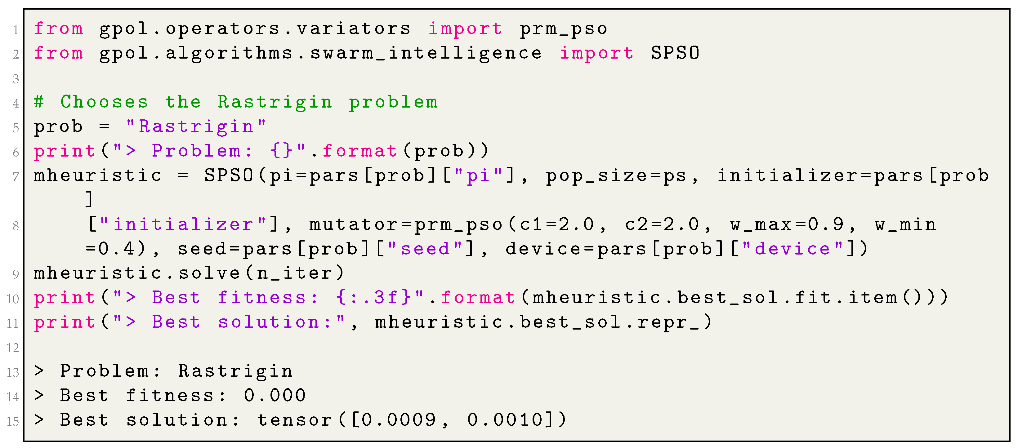These are implemented as SPSO and APSO classes. The former extends PopulationBased, whereas the latter extends SPSO; both require an additional parameter, called v_clamp which allows one to bound represents the velocity vector to foster the convergence, as suggested in [53]. The solve method for SPSO and APSO reflects the underlying algorithmic logic which guides the search-procedure. Additionally, both classes implement a private method, called _update, which efficiently encapsulates step number 2 from the procedural steps of S-PSO and A-PSO, and constitutes the main difference between the two classes. In the scope of swarm intelligence, the force-generating mechanism that yields ${\overrightarrow{x}}_{(p,i)}$ (and essentially, dictates how how the candidate solutions will “move” across S) is encapsulated in the mutator function, and is provided as a parameter during algorithms’ instantiate-generation. In this sense, the function force-generating function is completely abstracted from the PSO algorithm, meaning that the user can easily personalize it with any other update-rule, if the interface is respected.

Appendix B.7 demonstrates how to create an instance of SPSO and apply it in different problem solving.

4. Operators

This library provides a broad range of operators that can be classified into three main groups, each stored as a module in a package called operators: the initialization (initializers), the selection (selectors), and the variation (variators) groups. A flexible implementation allows the same operators to be used across different metaheuristics, and in some cases, optimization problems. Thus, the operators must follow a predefined signature. The following subsections present the operator groups.

4.1. Initialization

The purpose of an initialization operator, from now on called the “initializer”, is to create an initial point in search space S of a given problem’s instance. From the definition, one can easily derive that these kinds of operators are problem-specific, as such, their execution needs the problem context formalized by S itself. Given this rationale, all the initializers implemented in this library are functions that receive at least the sspace and the device parameters (the latter to indicate on which processing device the solutions should be allocated); this is the case of SP algorithms, such as RandomSearch, HillClimbing, and SimulatedAnnealing. In the case of PB algorithms, an initializer has one additional parameter, called n_sols, which represents the population’s/swarm’s size. Such branching is necessary because, by definition, not all the PB initialization operators can generate one solution. Additionally, it allows the user to encapsulate a computationally more efficient generation of a set of initial solutions.

The module called initializers implements all the necessary initialization functions that can be used to solve any kind of problem admitted in this library.

Table 1. Descriptions of the initializers implemented.

Function	OP Type	MH	Description
prm_rnd_vint(lb, ub)	Knapsack	SP	vector generated under ∼$U\{lb,ub\}$
prm_rnd_mint(lb, ub)		PB	matrix generated under ∼$U\{lb,ub\}$
rnd_vshuffle	TSP	SP	permutation vector of cities
rnd_mshuffle		PB	permutation matrix of cities
rnd_vuniform	Continuous	SP	vector generated under ∼$U(lb,ub)$
rnd_muniform		PB	matrix generated under ∼$U(lb,ub)$
grow	SML-IP	SP	LISP tree created with Grow method [36]
prm_grow(sspace)
full			LISP tree created with Full method [36]
prm_full(sspace)
rhh		PB	list of LISP trees created with RHH [36]
prm_edda			list of LISP trees created with EDDA [57,58]

enumerates the initializers and indicates for which problem types these can be applied. From the table, the column Function represents the name of the implemented initialization function, OP type stands for the type of problem for which the respective function can be applied, MH represents whether the function was designed for a SP or PB metaheuristic, and finally, the column Description briefly describes each function.

As will be shown with more detail in Section 4.3, the library’s interface restricts the variation operators’ parameters to solutions’ representation (only). However, some of the GP’s variation operators generate random trees, such as the sub-tree mutation and the geometric semantic operators, and their enclosing scope does not contain enough information to perform the variation operation. To remedy this situation, Python closures are used to provide the variation functions with the necessary outer scope for the trees’ initialization (the search space). In this sense, the prefix “prm” (means parametric), for grow and full, represents the usage of a Python closure; for example, prm_grow is a special adaptation of the grow function that accepts as a parameter the S of a given problem’s instance. Additionally, this solution allows one to have a deeper control over the operators’ functioning—an important feature for the research purposes.

4.2. Selection

A portion of the existing population is selected to breed a new generation. Individual solutions are selected through a fitness-based process, through which better solutions (as measured by a fitness function) are typically more likely to be selected. Certain selection methods rate the fitness of each solution and preferentially select the best solutions. Other methods rate only a random sample of the population, as the former process may be time-consuming.

The purpose of a selection operator, from now on called the “selector”, is to select a subset of individuals from the parent population for the sake of “breeding” (simulated through the application of the variation operators, to be described in the next subsection). The parent selection is traditionally fitness-based (i.e., the likelihood of selecting an individual increases with its fitness). From the definition, one can already deduce that this kind of operator is (1) specific to the population-based metaheuristics, namely, the branch of evolutionary algorithms, and (2) typically representation-free, as such they do not depend on a specific type of problem. Given this rationale, all the selectors implemented in this library are functions that receive the reference to the parent population (an object of type Population from where to select an individual), and the optimization’s purpose (min_).

The module called selectors implements all the necessary selectors that can be used to solve any kind of problem admitted in this library.

Table 2. Descriptions of the selectors implemented.

Function	MH Type	Description
prm_tournament(pressure)	{GA, GSGP}	tournament selection of one individual
roulette_wheel		roulette wheel selection of one individual
rank_selection		rank-based selection of one individual
rnd_selection		selects one individual at random
prm_dernd_selection(n_sols)	DE	random selection of n_sols vectors

enumerates them and describes their functionality. More specifically, the column Function represents the name of the implemented initialization function; MH type identifies the type of metaheuristic for which the selector can be used; and finally, the column Description briefly describes each function.

As previously mentioned, all the selectors in this library accept two parameters: Population and min_. This configuration suits the majority of selectors. However, some operators require a larger enclosing scope; this is the case of tournament selection which requires an additional parameter: the selection’s pressure. To remedy this situation, Python closures are used to provide the selectors with the necessary outer scope. In this sense, the prefix “prm” in prm_tournament represents the usage of a Python closure which allows the user to parametrize the necessary pressure. Similarly, prm_dernd_selection receives an outer parameter called n_sols, which tells the function how many random vectors to select for the sake of the DE’s mutation. In this sense, the parameter n_sols allows for easily including different DE mutation strategies, as these might include different amounts of random vectors.

4.3. Variation Functions

The functioning of an metaheuristic directly depends on the procedural steps that control the candidate-solutions’ “movement” across search space S and between iterations i to $i+1$. These steps fully characterize the algorithm and its logic. However, there is another important component, that can be abstracted from the algorithms’ high-level steps: the operators. In the evolutionary algorithms, these can be the crossover, the mutation, and in some cases, the reproduction. In swarm intelligence, these are the force-generating equations that update the particles’ positions. In a local search, these are the neighbor-generating functions (also known as the neighborhood functions). This library provides a wide range of different variation operators for different types of metaheuristics and optimization problems. Moreover, we formalize a connection between the local search and the evolutionary branches of metaheuristics, smoothing the distinction between the EA mutation and the LS neighbor-generating operators. That is, the mutation functions used with GA, GP, or GSGP can be directly used for HC or SA. In our opinion, this decision enhances the flexibility, the reliability and the objectiveness of the direct comparison between EAs and LSs.

Given the aforementioned equivalency between EA mutation and LS neighborhood generation, the variation functions implemented in this library are classified into three types: the mutators, the crossovers, and the force-generating equations, the latter being specific to PSO. In GPOL, the variation operators act directly upon solution representations and return new, potentially improved, representations. For this reason, the conventional signature for the EAs’ variation operators and their output is the following:

• mutator(repr_), where repr_ stands for the representation of a single parent solution to be mutated, and the function returns the mutated copy of repr_;
• crossover(p1_repr, p2_repr), where p1_repr and p2_repr stand for the representations of two different parents, and the function returns two modified copies of p1_repr and p2_repr.

There is one interesting saying, frequently attributed to General MacArthur: “The rules are mostly made to be broken”. This is also the case of this library, as there are several exceptions regarding the aforementioned guidelines. Some operators require more than the aforementioned parameters to work out. For example, the ball mutation, typically used in continuous optimization, requires two additional parameters: the probability of applying the operator at a given position of the solution’s representation and the radius of the “ball.” This kind of exception is generally handled by means of Python closures, which provide all the necessary outer scope for the mutation operators. Similarly, not all the variation operators will have the same return. A notorious example of such an exception is the efficient implementation of GSOs: as the computation is performed semantics, to reconstruct the trees after executing the evolutionary process, one needs to keep track of the random trees generated during the operators’ application. For this reason, GSOs will also output the random trees to allow the efficient implementation as proposed in [26,45].

Although DE can be classified as an EA, some of the structural differences did not allow us to maintain the aforementioned guidelines for its signature and output; as such, the variation operators for DE will follow a different convention. Several alternative mutation strategies were proposed in the literature and their enumeration and descriptions can be found in [49,50]. Most of them are present in this library. The list below presents the signatures for the DE mutation and crossover operators and their output.

• DE/rand/N: One type of DE mutation that creates the donor vector (the mutant) from adding N weighted differences between $2N$ randomly selected parent vectors to another ${(2N+1)}^{th}$ random parent. The underlying weights are provided by to the functions through the Python closures. Thus, the signature of these functions simplifies to mutator(parents), where parents is a collection containing $(2N+1)$ randomly selected parents. The function returns one donor vector (the mutant).
• DE/best/N: Another type of DE mutation that creates the donor vector from adding N weighted differences between $2N$ randomly selected parent vectors to the best parent at the current iteration. Similarly to DE/rand/N, the weights are provided through the Python closures. The signature of these functions simplifies to mutator(best, parents), where best stands for the best parent and parents contains $(2N+1)$ random parents. The function returns one donor vector (the mutant).
• DE/target-to-best/1: Another type of DE mutation that creates the donor from summing the target vector’s (the current parent) two weighted differences: one between two randomly selected parents and one between the best parent and the target vector itself. Similarly to the previous operators, the weights are provided through the Python closures. The signature of these functions simplifies to mutator(target, best, parents), where target stands for the current parent, best stands for the best parent and parents contain two random parents. The function returns one donor vector (the mutant).
• crossover(donor, target), where donor and target stand for the representations of two different vectors: The donor vector, generated by means of mutation, and the target vector (current parent). The function returns the trial vector (result of the DE’s crossover).

Regarding PSO, the force-generating equations must receive the following four parameters: the position of the particle p in S (pos_p), the velocity vector from the previous iteration (v_p), the best-so-far location found by p (lBest_p), the best-so-far location found by the swarm (gBest), and finally, the current and the maximum number of iterations (being the latter two necessary for the inertia’s update). All the remaining parameters must be provided in the outer scope by means of Python closures. In this sense, the prefix “prm” in prm_pso represents the usage of a closure that allows the user to specify the necessary social (c1) and cognitive (c2) factor weights, along with the inertia’s range (w_max and w_min).

The module called variators implements all the necessary variation operators that can be used to solve any kind of problem admitted in this library.

Table 3. Descriptions of the variators implemented.

Function	OP	MH	Description
one_point_xo	Knapsack01	GA, HC, SA	one point crossover
prm_n_point_xo(n)			n point crossover
binary_flip			flips a randomly selected value ($\overrightarrow{x_i}=!\overrightarrow{x_i}$)
prm_ibinary_flip(prob)			$\overrightarrow{x_i}=!\overrightarrow{x_i}$ with $P\left(M_i\right)=prob$
prm_rnd_int_ibound(prob, lb, ub)	KnapsackBounded		$\overrightarrow{x_i}\sim U\{lb,ub\}$ with $P\left(M_i\right)=prob$
partially_mapped_xo	TSP		partially mapped crossover
prm_iswap_mtn(prob)			random swap of the $i\mathrm{th}$ element with $P\left(M_i\right)=prob$
geometric_xo	Continuous Function		geometric crossover [59]
prm_iball_mtn			ball mutation [59]
de_binomial_xo(prob)		DE	binomial crossover for DE
de_exponential_xo(prob)			exponential crossover for DE
de_rand			DE/RAND/N mutation scheme
de_best			DE/BEST/N mutation scheme
de_target_to_best			DE/TARGET-TO-BEST/N mutation scheme
prm_pso(c1, c2, w_max, w_min)		A-PSO	PSO’s force-generating equation (also known as update rule)
swap_xo	SML-IP	{GA, HC, SA}	standard GP’s crossover (also known as a swap crossover)
prm_gs_xo(initializer, device)			GSC that works upon tree-like representations [38]
hoist_mtn			hoist mutation
prm_point_mtn(sspace, prob)			point mutation
prm_subtree_mtn(initializer)			standard GP’s mutation (also known as a sub-tree mutation) [38]
prm_gs_mtn(initializer, ms)			GSM that works upon tree-like representations
prm_efficient_gs_xo(X, initializer)		GSGP	efficient GSC that works upon semantics [45]
prm_efficient_gs_mtn(X, initializer, ms)			efficient GSM that works upon semantics [45]

enumerates them operators and describes their functionalities. More specifically, the column Function represents the name of the implemented initialization function; MH type identifies the type of metaheuristic for which the selector can be used; and finally, the column Description briefly describes each function.

5. Solutions

The purpose of a search algorithm (SA) is to solve a given problem. The search process consists of traveling across the search space S in a specific manner (which is embedded in the algorithm’s definition). This “tour” consists of generating solutions from S and evaluating them through f. In this context, a solution can be seen as the essential component in the mosaic composing this library. Concretely, we implement a special data structure, called Solution, which encapsulates the necessary attributes and behavior of a given candidate solution, specifically the unique identification, the representation in the light of a given problem, the validity state in the light of S, and the fitness value(s) (which can be several, depending if data partitioning was used). To ease the library’s necessity for flexibility, in this release, the solution’s representation can take one of two forms: either a list or a tensor (torch.Tensor). The former relates to GP trees, and the latter relates to the remaining array-based representations.

Some algorithms manipulate whole sets of solutions at a time to perform such a search. For this reason, in the scope of this library, a special class was created to encapsulate the whole population of candidate solutions efficiently. Specifically, to avoid redundant generations of objects to store a set of solutions, their essential characteristics will be efficiently stored as a limited set of macro-objects, all encapsulated in the class Population.

6. Conclusions

We presented GPOL: a new Python library for numerical optimization that unites, under the same “umbrella”, a wide range of stochastic iterative search algorithms and optimization problems. The library’s flexible and modular implementation provides the user with a controlled and intuitive environment for benchmarking. The efficient implementation and optional GPU acceleration make the library suitable for heavy computational tasks. Moreover, the library provides for the implementation of several state-of-the-art algorithms and is flexible enough to incorporate new techniques and approaches easily. This contribution should be useful for the scientific and practitioner communities.