A Genetic Programming Approach for Economic Forecasting with Survey Expectations

Abstract

We apply a soft computing method to generate country-specific economic sentiment indicators that provide estimates of year-on-year GDP growth rates for 19 European economies. First, genetic programming is used to evolve business and consumer economic expectations to derive sentiment indicators for each country. To assess the performance of the proposed indicators, we first design a nowcasting experiment in which we recursively generate estimates of GDP at the end of each quarter, using the latest business and consumer survey data available. Second, we design a forecasting exercise in which we iteratively re-compute the sentiment indicators in each out-of-sample period. When evaluating the accuracy of the predictions obtained for different forecast horizons, we find that the evolved sentiment indicators outperform the time-series models used as a benchmark. These results show the potential of the proposed approach for prediction purposes.

1. Introduction

The pandemic has caused a disruption in the evolution of macroeconomic aggregates. Consequently, the estimation of upcoming events becomes one of the fundamental objectives of economic analysis, especially in periods of high uncertainty, such as the current period. Recent trade disputes and growing investor concerns about the global economic outlook have led the International Monetary Fund (IMF) to downgrade global growth projections for 2020, which have their lowest levels since the 2008 financial crisis [1]. In this context, agents’ expectations about future economic conditions are a key feature in macroeconomic forecasting.

Expectations are not directly observable. Consequently, agents’ expectations tend to be elicited via surveys. Survey expectations present several advantages over experimental expectations, such as the following: (a) they are based on the knowledge of respondents operating in the market, (b) they provide detailed information about a wide range of economic variables, and (c) they are available ahead of the publication of official quantitative data. These features make them very useful for prediction.

One of the main sources of expectation information are economic tendency surveys (ETS). In ETS, respondents are asked whether they expect variables to rise, fall, or remain unchanged. Some of the most well-known ETS are collected by the University of Michigan, the Federal Reserve Bank of Philadelphia, the Organisation for Economic Co-operation and Development (OECD), and the European Commission (EC). In 1961, the EC launched the Joint Harmonised Programme of Business and Consumer Surveys with the aim of unifying the survey methodologies in the member states of the European Economic Community, now the European Union (EU), allowing comparability between countries.

Survey responses from ETS are commonly used to design composite confidence and sentiment indicators, such as the ifo World Economic Climate Index, the University of Michigan Consumer Confidence Index or the Purchasing Managers’ Index calculated by the Markit Group. The EC constructs business and consumer confidence indicators as the arithmetic mean of a subset of predetermined survey expectations.

The selection of variables for construction of confidence indicators is fundamentally determined by their fit to a reference series. Economic relationships between variables change over time and require periodic overhaul [2]. Therefore, in this study, we propose a machine-learning method for the generation of economic sentiment indicators that allows both an automated variable selection procedure and an update of the relationships between the selected variables. One can refer to [3,4] for a comprehensive assessment of the automated selection procedures.

The proposed approach allows the determination of an optimal combination of expectations that minimizes a set loss function. The obtained expressions differ from the confidence indicators constructed by the EC in the following ways: (a) they are based on information from all the available variables of each survey, (b) they select expectations with the highest forecasting power and their optimal lag structure, (c) they capture the existing non-linear relationships between survey expectations, and (d) they generate direct estimates of economic growth. In [5], the authors found evidence of the non-linear relationship between expectations and economic growth.

The objective of the paper is threefold. First, we aim to provide practitioners with easy-to-implement business and consumer confidence indicators. To this end, we have used all the variables contained in the industrial and consumer surveys conducted by the EC for 19 EU states and for the euro area (EA). With this information, we generated country-specific confidence indicators that estimate the GDP growth rate expected by firms and consumers. Secondly, because the algorithm selects the expectational variables with the highest predictive capacity, including the number of lags, we evaluate the relative importance of the variables in each survey, as well as their lag structure.

Finally, we assess the forecasting performance of the generated indicators. On the one hand, we compare them to the confidence indicators constructed by the EC in a nowcasting exercise. On the other hand, we design a recursive out-of-sample forecasting experiment in which we iteratively re-compute the indicators to predict economic growth. The obtained forecasts are then compared to univariate time-series models that are used as a benchmark.

The proposed methodology is based on genetic programming (GP), which is a soft computing search technique based on the application of evolutionary algorithms. GP simultaneously evolves the structure and the parameters of expressions, allowing formalization of the interactions between the variables that best fit a reference series. This approach is especially useful in situations where the exact functional form of the solution is not known in advance, such as the present one, where there is no a priori combination of survey expectations that best tracks economic growth.

GP has been successfully used as a tool for automatic problem-solving in areas such as image processing [6], but very seldom for macroeconomic modelling and forecasting [7,8,9,10,11]. In this study, we fill this gap by applying GP to the estimation of free-form regressions that link economic growth with survey expectations in order to generate country-specific machine-learning sentiment indicators. We design an independent experiment for each country and for each type of survey, obtaining data-driven confidence indicators that allow us to independently monitor economic growth dynamics from both the demand and the supply sides of the economy.

The rest of the paper proceeds as follows: the next section describes the methodological approach and the experimental setup. In Section 3, we present the obtained indicators. In Section 4, we assess the performance of the evolved confidence indicators in a nowcasting exercise. In Section 5, we perform an iterative forecasting experiment. Finally, Section 6 concludes the paper.

2. Methods

GP is a heuristic search technique based on the evolution of programs. This optimization approach represents programs in tree structures that learn and adapt by changing their size, shape, and composition of the models. As opposed to conventional regression analysis, which is based on a certain ex-ante model specification, GP-based symbolic regression (SR) searches for relationships between a given set of variables and evolves the functions until it reaches a solution, which in our case corresponds to the algebraic expression that best fits the data. One can refer to [12] for a comparative analysis of the metaheuristic optimization algorithms.

GP simultaneously evolves the structure and the parameters of the expressions. This feature provides a quick overview of the most relevant interactions between the variables of the system and can help to identify new unknown links. As a result, due to its suitability for finding patterns in large datasets and handling complex modelling tasks, this empirical modelling approach is beginning to be used in more and more applications in different scientific fields, from lung cancer prediction [13] and automatic skin cancer image classification [14], to a wide range of engineering applications [15,16,17,18,19,20]. A large part of the applications is related to complex optimization problems [21,22,23] and predictive tasks in different fields [24,25].

Although GP-based SR was first used as a means to assess the non-linear interactions between price level, gross national product, money supply, and the velocity of money [26], applications of GP in macroeconomics have been very limited since then. Using a similar procedure, in [27], the authors identified interactions between economic indicators in order to estimate the evolution of prices in the US. In [28], the authors assessed the performance of different model selection approaches, including GP, in an out-of-sample forecasting exercise to predict the growth rates of quarterly GDP and monthly inflation. Similarly, in [29], the authors used GP to track GDP growth by combining ten science and technology factors. In [30], the authors applied GP in a vector error correction model for macroeconomic forecasting. One can refer to [31] for a review of the application of GP to economic modelling.

Most of the applications of evolutionary computation in economics have been made in finance [32]. In [33], the authors used a genetic algorithm to predict the financial failure of firms. In [34], the authors applied genetic algorithms to optimize the signals generated by technical trading tools. However, most of the works focus on the prediction of exchange rates or stock price trends (e.g., [35,36,37,38,39,40]). One can refer to [41] for a recent review of the applications of genetic algorithms to forecasting prices of commodities. For a review of the applications of evolutionary algorithms for financial forecasting, one can refer to [42].

Evolutionary computation is based on the application of the principles of the theory of natural selection to an iterative optimization problem. The implementation of GP starts by the creation of an initial random population of M individuals (functions or programs), from which the algorithm selects the fittest ones (parents). In order to guarantee diversity in the population, we used the size three tournament method as the strategy for the selection of parents for replacement, meaning that the best two out of three individuals randomly selected are finally mated.

Genetic operators (reproduction, crossover and mutation) are applied to the selected parents (N). Reproduction results in the copying of the function; crossover consists of exchanging random parts of selected pairs; and mutation involves substitution of some random part of a function with some other part.

In each successive simulation (generation), a new and fitter offspring is generated. The fitness of each member of the population is evaluated by a loss function. Operations are recursively applied to the new generations until a stopping criterion is reached. The recursion stops when some individual program reaches a predefined fitness level or when the process reaches a given number of generations (Ng). The output of this process consists of the best individual function from all generations.

In our case, we generated a first random population of 70,000 functions, and selected the best 10,000 individuals according to the obtained mean square error. We set a maximum number of 100 generations as the termination criterion.

In this study, we implemented GP to generate composite indicators that capture the optimal combinations of survey variables that best track the actual evolution of economic growth. Formally, the objective of the algorithm is to infer a functional relationship from a set of observations, such that the inferred function $f\left(x_i\right)$ is as near as possible to the reference series in the Euclidean distance sense, where index $i=1,\dots , M$ denotes the sample size. The search process is characterized by a trade-off between accuracy and simplicity. To limit the complexity of the resulting expressions, the set of functions is restricted to the four elementary mathematical operations (addition, subtraction, product, and division). One can refer to [43] for a detailed study on the effect of the choice of function sets on the generalization performance of SR models.

With the aim of further restricting the complexity of the resulting functional forms, we additionally introduced regularization terms in the slope and curvature of the inferred functions. For a justification of the need to regularize, one can refer to [44]. We used the Distributed Evolutionary Algorithms in Python (DEAP), developed by [45].

Finally, by way of synthesis, we want to highlight some of the advantages and disadvantages of the proposed methodology. As for the advantages, we want to note that, unlike the confidence indicators constructed by the EC, the obtained evolved expressions proposed in the present study generate direct estimates of economic growth, which are based on information from all the available variables of the industry and consumer surveys. Additionally, the proposed approach automatically selects the expectational variables with the highest forecasting power and their optimal lag structure, which is predefined in the design of the experiment, ranging in our case from one to a maximum of four quarters. Finally, the proposed approach detects existing non-linear relationships between survey expectations and allows them to be modelled.

Regarding the limitations of the proposed methodology, we want to note that due to the empirical nature of the proposed approach, the evolved expressions lack any theoretical background. Another limitation of the proposed approach is that, as opposed to standard regression, the significance of the parameters obtained in SR cannot be assessed. Finally, given that GP-based SR is a stochastic, high-variance algorithm, its sensitivity to changes in training data can be a drawback for certain practical applications. In this sense, the implementation of preliminary sensitivity analyses through Monte Carlo simulations and the incorporation of prior knowledge are ways to mitigate this effect.

3. Evolved Indicators

This study matches two sources of information, official quantitative GDP data and firms’ and consumers’ qualitative expectations about a wide array of variables. Regarding the quantitative information, we used seasonally adjusted year-on-year growth rates of GDP provided by Eurostat. With respect to agents’ expectations, we used all monthly and quarterly data from the Joint Harmonised EU Industry and Consumer surveys conducted by the EC (see

Table A1. Survey indicators.

Industry Survey
Monthly questions
B1—Production trend observed in recent months
B2—Assessment of order-book levels
B3—Assessment of export order-book levels
B4—Assessment of stocks of finished products
B5—Production expectations for the months ahead
B6—Selling price expectations for the months ahead
B7—Employment expectations for the months ahead
Quarterly questions
B8—Assessment of current production capacity
B9—New orders in recent months
B10—Export expectations for the months ahead
B11—Current level of capacity utilization (%)
B12—Competitive position domestic market
B13—Competitive position inside EU
B14—Competitive position outside EU
Consumer survey
Monthly questions
C1—Financial situation over last 12 months
C2—Financial situation over next 12 months
C3—General economic situation over last 12 months
C4—General economic situation over next 12 months
C5—Price trends over last 12 months
C6—Price trends over next 12 months
C7—Unemployment expectations over next 12 months
C8—Major purchases at present
C9—Major purchases over next 12 months
C10—Savings at present
C11—Savings over next 12 months
C12—Statement on financial situation of household
Quarterly questions
C13—Intention to buy a car within the next 12 months
C14—Purchase or build a home within the next 12 months
C15—Home improvements over the next 12 months

in the Appendix A). Monthly survey indicators were aggregated on a quarterly basis and can be freely downloaded at the website of the EC.

The sample period is from 2003.Q1 to 2020.Q1. The last seventeen quarters were used as the out-of-sample period to evaluate forecast accuracy. We focused on 19 European countries, including Austria (AT), Belgium (BE), Bulgaria (BG), the Czech Republic (CZ), Denmark (DK), Finland (FI), France (FR), Germany (DE), Greece (EL), Hungary (HU), Italy (IT), the Netherlands (NL), Poland (PL), Portugal (PT), Romania (RO), Slovenia (SI), Spain (ES), Sweden (SE) and the United Kingdom (UK) and the EA.

In both the industry survey and the consumer survey, respondents are asked about their expectations regarding future developments and their perceptions about past and present changes. In either case, the results are presented as balance series, which are obtained from the percentage of positive replies minus the percentage of negative replies. The EC publishes one composite indicator for each survey, including the industry confidence indicator (ICI) for the industry survey and the consumer confidence indicator (CCI) for the consumer survey. Both indicators are obtained from the arithmetic mean of the balance series of a subset of questions.

In this section, we present the industry and consumer confidence indicators obtained for each country and for the EA after the evolutionary process. We ran two independent experiments for each country. In the first one, we linked GDP growth to the industry survey indicators. In the second one, we linked GDP growth to consumer survey indicators. The outputs of the first set of experiments are country-specific evolved industrial confidence indicators that generate estimations of firms’ expectations of economic growth (Exp.IND), while the outputs of the second set of experiments are evolved consumer confidence indicators for each country that yield estimations of households’ expectations of the evolution of economic activity (Exp.CONS). The obtained industrial and consumer confidence indicators are respectively presented in

Table 1. Evolved industrial confidence indicators.

Country	Evolved Industrial Confidence Indicators
Austria	$0.10\ast B{1}_t+0.02\ast B{10}_{t-2}+0.01\ast B{1}_{t-2}+0.01\ast B{2}_t-0.01\ast B{4}_{t-4}$
Belgium	$\frac{B{11}_{t-1}+B{11}_{t-2}-B{14}_t\ast B{5}_{t-1}+B{8}_{t-3}}{B{11}_{t-3}+B{8}_t}$
Bulgaria	$10.01\ast \frac{B{1}_t+B{5}_{t-2}}{B{11}_t }$
Czech Republic	$0.10\ast \frac{-B{1}_{t-2}\ast \left(B{8}_{t-2}\right)+\left(B{2}_{t-2}+\left(B{5}_t-10.01\right)\ast B{8}_{t-2}\right)\ast \left(B{5}_t+B{5}_{t-2}\right)}{B{2}_{t-2}+\left(B{5}_t-10.01\right)\ast \left(B{8}_{t-2}\right)}$
Denmark	$0.10\ast \frac{-B{1}_t+\left(B{1}_t+20.01\right)\ast \left(B{1}_t+B{10}_{t-3}\right)}{B{1}_t+20.01}$
Finland	$0.05\ast B{1}_t+0.10\ast B{5}_t+0.05\ast B{9}_{t-1}-1.01$
France	$0.10\ast B{10}_t+0.10\ast B{11}_{t-1}-0.10\ast B{11}_{t-4}+1.01$
Germany	$\frac{0.10\ast \left(B{10}_{t-1}\right)\ast \left(B{1}_t+B{10}_{t-1}+B{14}_{t-2}\right)+1.01}{B{10}_{t-1}}$
Greece	$\frac{0.23\ast B{1}_t\ast \left(B{11}_t \right)\ast \left(B{11}_{t-4}\right)-B{11}_{t-4}-\left(B{1}_{t-4}\ast B{9}_t-B{1}_t \right)\ast \left(B{11}_{t-4}\right)}{\left(I{11}_t \right)\ast \left(I{11}_{t-4}\right)}$
Hungary	$\frac{-0.51\ast B{1}_{t-4}+13.10\ast B{5}_t-B{6}_{t-2}\ast B{7}_{t-1}}{B{11}_t }$
Italy	$\frac{-B{1}_{t-3}+B{2}_t+B{5}_{t-1}+2.01\ast B{9}_t}{B{8}_{t-3}}$
Netherlands	$0.01\ast B{2}_{t-1}+0.11\ast B{5}_t+0.10\ast B{5}_{t-1}+0.01\ast B{9}_{t-1}$
Poland	$\frac{0.28\ast B{9}_t}{0.28\ast \frac{B{11}_{t-3}}{B{3}_{t-4}}+B{8}_{t-3}+4.24}+3.52$
Portugal	$0.10\ast B{12}_t-0.10\ast B{14}_{t-4}+0.10\ast B{4}_{t-3}+0.10\ast B{5}_t+0.10\ast B{5}_{t-1}+0.23$
Romania	$0.31\ast B{5}_{t-1}-\frac{0.92}{\left(\frac{B{2}_{t-1}+3.31}{B{11}_{t-4}}\right)\ast \left(B{5}_{t-1}\right)}$
Slovenia	$\frac{0.10\ast B{11}_{t-3}-0.10\ast B{1}_{t-1}+0.10\ast \left(B{11}_{t-3}\right)\ast \left(B{10}_{t-1}+B{2}_t+B{4}_{t-4}\right)-0.05}{B{11}_{t-3}}$
Spain	$0.10\ast B{1}_t+0.10\ast B{4}_{t-3}+0.10\ast B{5}_{t-2}+0.10\ast B{5}_{t-4}+0.38$
Sweden	$0.10\ast B{5}_{t-2}-0.10\ast B{6}_{t-1}+0.10\ast B{9}_t$
UK	$-0.04\ast B{14}_{t-2}+0.10\ast B{5}_t+0.41$
EA	$0.10\ast B{1}_t+0.10\ast B{10}_{t-1}+0.10\ast B{4}_{t-2}$

and

Table 2. Evolved consumer confidence indicators.

Country	Evolved Consumer Confidence Indicators
Austria	$\frac{2.01\ast C{11}_t+C{12}_{t-2}+2.01\ast C{4}_{t-2}-C{5}_{t-3}-C{9}_{t-2}}{C{12}_{t-1}}$
Belgium	$\frac{C{13}_{t-3}+C{14}_{t-1}+C{2}_{t-2}\ast C{3}_{t-2}}{C{10}_t+C{13}_{t-3}}$
Bulgaria	$\frac{0.10\ast C{6}_{t-1}\ast \left(C{10}_t+2.01\ast C{7}_t\right)-\left(C{10}_t+C{7}_t\right)\ast C{14}_{t-2}}{C{14}_{t-2}}$
Czech Republic	$0.10\ast \left(-C{15}_{t-2}+C{3}_t+C{8}_t-C{9}_{t-4}\right)$
Denmark	$\frac{C{3}_t\ast C{7}_{t-2}+\left(C{11}_{t-1}\right)\ast \left(C{12}_{t-3}+C{3}_t+C{4}_{t-3}-C{5}_{t-2}\right)}{\left(C{11}_{t-1}\right)\ast \left(C{12}_{t-3}\right)}$
Finland	$0.10\ast \frac{-C{15}_{t-4}\ast \left(C{3}_{t-2}\right)+\left(C{3}_t+C{8}_{t-4}\right)\ast \left(-0.50\ast C{8}_{t-4}+C{10}_{t-3}\ast C{3}_{t-2}\right)}{-0.50\ast C{8}_{t-4}+\left(C{10}_{t-3}\right)\ast \left(C{3}_{t-2}\right)}$
France	$2.06+\frac{0.15\ast C{13}_{t-3}}{C{3}_{t-1} }-\frac{1.85\ast C{1}_{t-4}}{C{13}_{t-2}-C{3}_{t-1}}$
Germany	$0.05\ast C{10}_{t-2}+0.04\ast C{4}_{t-1}-0.05\ast C{5}_{t-2}-0.05\ast C{7}_t+1.86$
Greece	$0.10\ast C{15}_{t-3}-0.10\ast C{2}_{t-1}+0.10\ast C{7}_t-1.01$
Hungary	$4.54+\frac{0.14\ast C{13}_t}{C{9}_t }+\frac{3.03\ast C{8}_t}{C{3}_t-C{13}_{t-1}}$
Italy	$\frac{C{6}_{t-4}\ast \left(-C{6}_{t-4}\right)}{ 11.01\ast C{6}_{t-4}-C{10}_{t-2}+20.50}$
Netherlands	$\frac{C{14}_{t-1}+C{1}_{t-2}+C{6}_{t-4}+2.01\ast C{7}_t+C{9}_{t-1}}{C{13}_{t-4}}$
Poland	$\frac{C{14}_{t-1}+C{14}_{t-2}+C{8}_{t-1}\ast C{9}_t+C{7}_t}{C{15}_{t-1}}$
Portugal	$\frac{C{14}_{t-1}+C{14}_{t-3}-C{2}_{t-2}+C{12}_{t-4}\ast C{5}_{t-3}-C{12}_{t-4}\ast C{2}_{t-2}}{C{13}_{t-4}}$
Romania	$\frac{4.65\ast C{10}_t-C{2}_t+C{13}_{t-4}+4.65\ast C{7}_t}{C{8}_t }$
Slovenia	$\frac{C{14}_{t-1}-C{6}_{t-1}+C{7}_t-2.01\ast C{8}_t}{C{11}_{t-2}}$
Spain	$\frac{-5.17\ast C{1}_t+0.76\ast C{15}_t-2.01\ast C{3}_{t-1}+4.44\ast C{9}_t}{C{11}_{t-3}}$
Sweden	$\frac{-C{4}_{t-1}+\left(C{8}_{t-1}\right)\ast \left(C{4}_{t-2}+C{1}_t+C{8}_{t-1}\right)}{\left(C{2}_{t-4}\right)\ast \left(C{8}_{t-1}\right)}$
UK	$\frac{C{14}_{t-3}\ast \left(C{14}_{t-3}-C{3}_t \right)-C{14}_{t-3}-C{3}_t\ast C{4}_{t-4}+C{8}_{t-1}}{\left(C{15}_t\right)\ast \left(C{14}_{t-3}-C{3}_t \right)}$
EA	$\frac{C{13}_{t-1}+C{13}_{t-3}+C{14}_{t-2}-C{2}_{t-2}\ast C{7}_t+3.78}{C{13}_{t-3}}$

.

When comparing the resulting indicators of industrial and consumer confidence, we observed that genetic algorithms generated more linear expressions for firms’ expectations. In most countries, the derived expression is a linear combination of several industry survey expectational variables, as opposed to evolved consumer confidence indicators, which are mostly non-linear and, include ratios and more complex interactions between survey indicators.

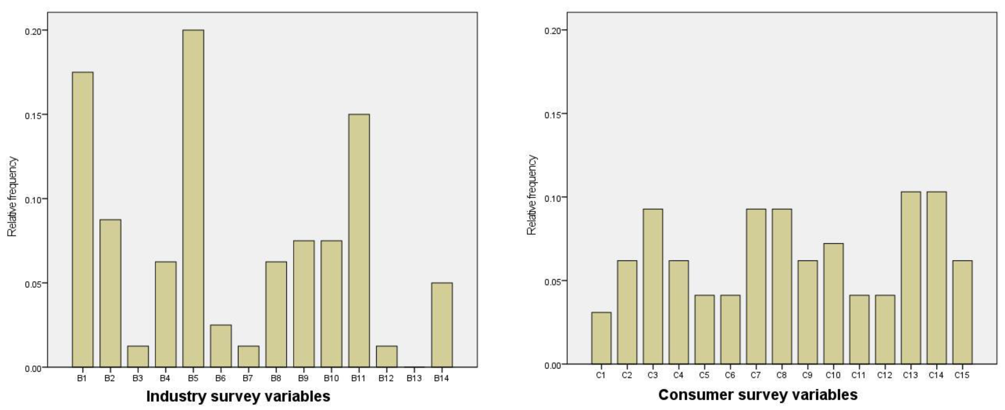
Regarding the lag structure, most variables tend to appear indistinctly lagged and contemporaneously, sometimes for the same country. In the case of the evolved consumer indicators, the financial and general economic situation over the last 12 months, as well as future unemployment expectations, mostly appear contemporaneously, in the same way as the observed production trend and new orders in recent months appear for the evolved industry indicators. The results of Table 1 and Table 2 are summarized in Figure 1.

In the bar chart, which shows the relative frequency with which each survey variable appears in the evolved expressions, we can observe that variable B5 from the industry survey (‘production expectations for the months ahead’) is the most frequent of the evolved industry confidence indicators. Regarding consumer expectations, variables C13 (‘intention to buy a car’) and C14 (‘intention to purchase a home in the next 12 months’) are the variables most frequently selected by the algorithm, both contemporaneously and lagged. We observe that the distribution of the industry survey variables shows less variance than that of the consumer survey variables, which is more flat-topped. It can be observed that each survey variable of the consumer survey appears at least 3 or 4 times in the evolved consumer confidence indicators; however, in the industry survey, production expectations appear 16 times, while other variables such as the ‘competitive position inside the EU’ do not appear for any country.

These obtained results suggest the predictive potential of production expectations in the industry. In the case of consumers, the intention to buy a car or a house are the variables with the highest informational content to capture economic growth dynamics. In [46], the authors found evidence of the predictive potential of variable B5 when evaluating the usefulness of expectations from the industry survey to improve the forecasting performance of time-series models in 26 European countries. It is also noteworthy that in spite of the leading properties of the variables contained in the consumer quarterly surveys, which are the most frequently selected variables by the algorithm, they have always been omitted by the EC in the construction of the official consumer confidence indicators.

4. Results

In this section, we examine the predictive performance of the proposed confidence indicators in tracking economic activity in a nowcasting exercise. We used the last 17 quarters (2016.Q1 to 2020.Q1) as the out-of-sample period, and the root mean square forecasting error (RMSFE) as a measure of forecast accuracy. First, we compared the forecasts obtained with the evolved confidence indicators (Exp.IND and Exp.CONS) to those obtained with the corresponding confidence indicators constructed by the EC, previously re-scaled (Cof.IND and Cof.CONS). Because the output of the evolved indicators is directly expressed as expected annual GDP growth rates, we re-scaled the indicators presented in expressions (1) and (2), by regressing the GDP growth of each country on the components of the indicators during the in-sample period (2003.Q1 to 2015.Q4).

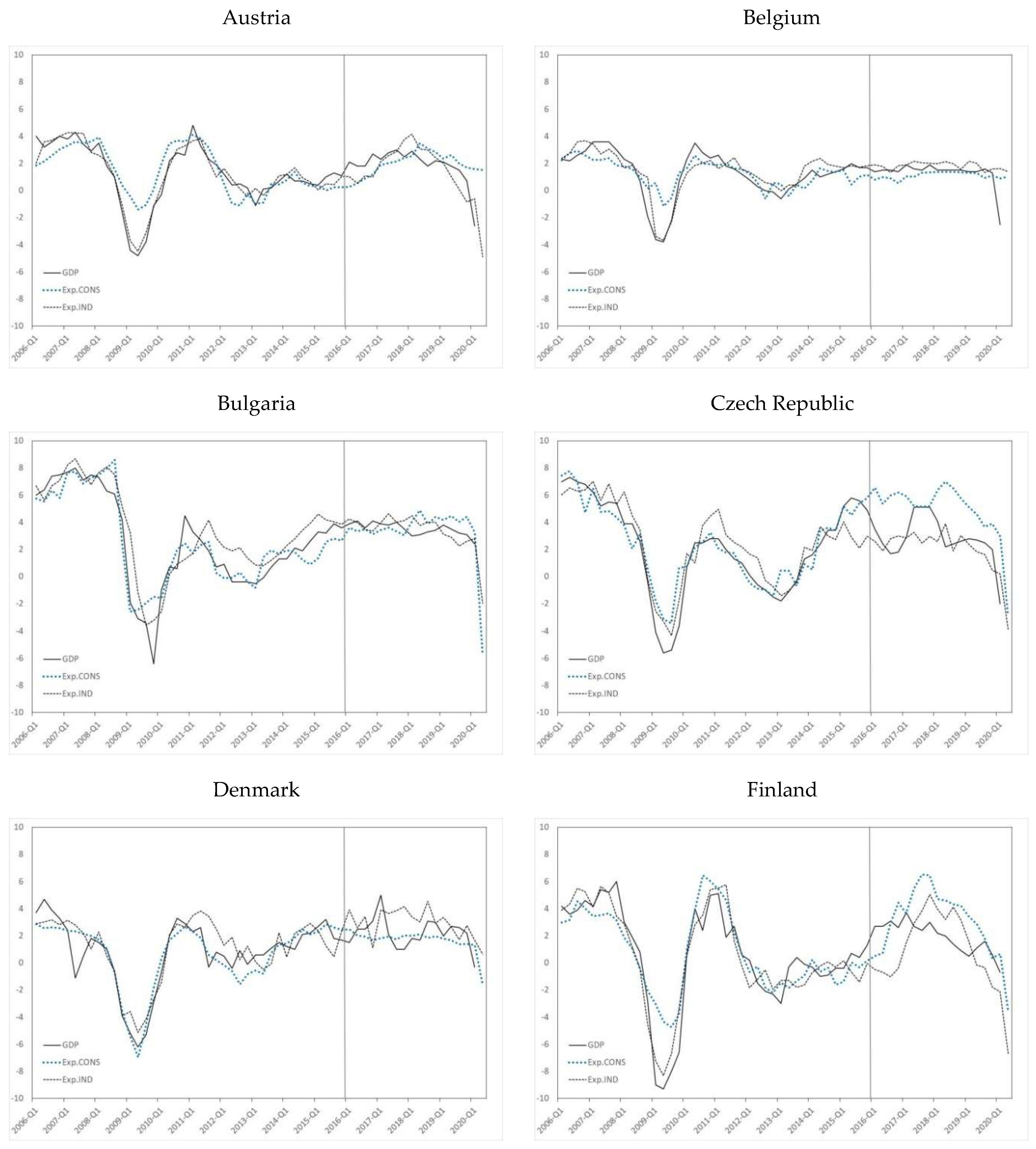
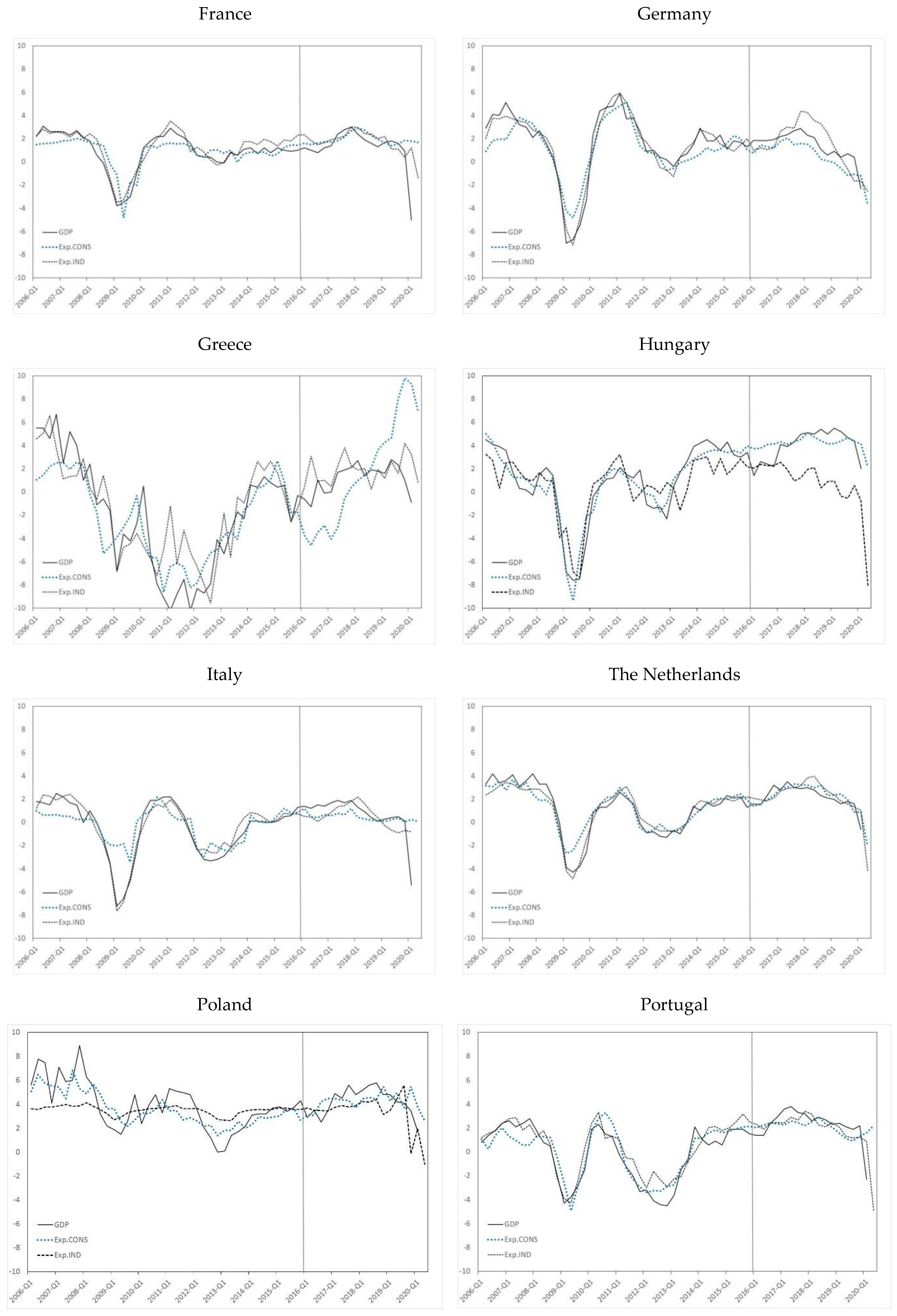
In Figure 2, we graphically compare the evolution of the two GP-generated indicators to that of the GDP of each country. The last seventeen quarters of the sample are used as the out-of-sample period, in which we use the results of the surveys to estimate the period-to-period economic growth prior to the publication of official data.

The EC publishes one composite indicator for the industry (ICI) and another one for households (CCI). Both indicators are obtained from the arithmetic mean of the balance series of a subset of questions.

$$IC{I}_t=\frac{B{2}_t+B{5}_t-B{4}_t}{3}$$

(1)

$$CC{I}_t=\frac{C{2}_t+C{4}_t+C{11}_t-C{7}_t}{4}$$

(2)

The in-sample OLS estimates of the weights of each of the components of the confidence indicators published by the EC allow us to compute the scaled confidence indicators that are directly comparable with the evolved confidence indicators. This experiment can be regarded as a nowcasting exercise, given that for each period, the indicators provide an estimation of the current state of the economy before the official figures are released, making exclusive use of the latest survey data published by the EC. For further discussion of nowcasting, one can refer to [47,48], and the references cited therein.

To test whether the reduction in accuracy is statistically significant, we computed the Harvey–Leybourne–Newbold (HLN) statistic [49], which is a modification for small samples of the Diebold–Mariano (DM) statistic [50]. Under the null hypothesis that there is no significant difference in precision, the statistic follows a Student’s-t distribution. A negative sign indicates that the second model has larger forecast errors. The results are presented in

Table 3. Forecast accuracy (RMSFE): Evolved indicators (Exp.) vs. Scaled indicators (Cof.)—Industry and consumer surveys and Aggregate expectations.

	Industry			Consumers			Aggregate
	Exp.IND	Cof.IND	HLN	Exp.CONS	Cof.CONS	HLN	Exp.Agg	Cof.Agg	Av.Cof.Agg	HLN(1)	HLN(2)
Austria	1.097	1.186	−0.324	1.383	1.651	−0.839	1.082	1.181	1.286	−0.370	−0.501
Belgium	1.089	0.954	−0.122	0.946	1.698	−4.978	0.994	0.937	1.085	−0.908	−3.151
Bulgaria	0.665	1.180	−2.611	0.851	0.918	−1.206	0.630	0.686	0.708	−0.253	−0.598
Czech Republic	1.393	1.639	−0.410	3.056	3.433	−0.392	1.489	1.580	1.910	0.046	−1.007
Denmark	1.643	1.516	0.272	1.189	1.084	0.686	1.147	1.120	1.235	0.463	−0.865
Finland	2.284	2.243	1.100	2.335	2.759	−1.391	2.087	2.241	2.366	0.196	−0.600
France	1.633	1.461	1.197	1.737	1.711	−1.137	1.648	1.448	1.485	0.576	0.204
Germany	1.244	1.808	−2.447	0.991	2.056	−2.120	0.943	1.653	1.655	−2.892	−3.219
Greece	1.838	1.757	0.334	4.386	4.248	0.799	2.472	2.733	2.839	−1.211	−1.734
Hungary	3.865	1.229	6.700	0.838	3.656	−6.518	0.870	3.547	2.237	−6.073	−4.721
Italy	1.373	1.167	0.711	1.522	1.568	−3.436	1.365	1.168	1.258	1.034	0.085
Netherlands	0.706	1.040	−2.311	0.592	2.265	−7.009	0.658	1.271	1.599	−3.196	−4.817
Poland	1.532	2.019	−2.469	1.116	2.486	−3.235	0.932	2.226	2.197	−5.065	−5.520
Portugal	1.009	1.113	−1.758	1.216	1.309	0.552	1.099	0.988	0.978	1.419	1.393
Romania	2.454	3.017	−1.349	1.506	1.268	1.325	1.517	1.884	1.921	−1.260	−1.612
Slovenia	1.505	1.355	0.425	3.989	2.203	2.606	1.505	2.203	1.408	−0.247	0.391
Spain	1.583	1.523	−1.235	2.357	1.629	0.973	1.677	1.493	1.494	0.139	0.010
Sweden	1.431	3.254	−3.018	0.952	1.520	−4.806	0.930	1.955	2.230	−4.150	−3.917
United Kingdom	0.895	1.232	−1.243	0.775	2.137	−6.045	0.747	1.425	1.467	−3.443	−3.912
Euro Area	1.025	1.093	−1.382	2.147	2.031	−0.329	1.238	0.804	0.981	0.598	−0.215

Notes: HLN denotes the Harvey–Leybourne–Newbold test statistic. Av.Cof.Agg denotes the average of the scaled confidence indicators for firms (Cof.IND) and consumers (Cof.CONS). HLN(1) compares Exp.Agg vs. Cof.Agg, while HLN(2) compares Exp.Agg vs. Av.Cof.Agg.

.

In Table 3, we can observe that in most countries, the lowest forecast errors are obtained using the evolved indicators contained in Table 1 and Table 2, although the difference in accuracy is not always statistically significant. For the industry, we obtained significantly lower forecast errors for Bulgaria, Germany, the Netherlands, Poland and Sweden; however, for consumers, we obtained these errors in Belgium, Germany, Hungary, Italy, the Netherlands, Poland, Sweden, and the UK. We also observed notable differences in accuracy between firms and households in countries such as the Czech Republic and Greece.

The EC weights the confidence indicators obtained for each of the surveys to calculate an aggregate index, the economic sentiment indicator (ESI). In [51,52], the authors showed that letting the aggregation weights of each component of the ESI be data-driven improves its forecasting performance. Hence, we next combined the estimations obtained from the evolved industry and consumer confidence indicators by means of constrained optimization. We used a generalized reduced gradient non-linear algorithm to minimize the summation of squared forecast errors and imposed the following two restrictions: (a) the sum of both weights must equal one, and (b) the weights must be equal to or larger than zero. The resulting weights are annexed in Appendix B (

Table A2. Relative weights of evolved expectations.

	Firms’ Expectations	Consumers’ Expectations		Firms’ Expectations	Consumers’ Expectations
Austria	0.948	0.052	Italy	0.824	0.176
Belgium	0.727	0.273	Netherlands	0.773	0.227
Bulgaria	0.389	0.611	Poland	0.441	0.559
Czech Republic	0.675	0.325	Portugal	0.464	0.536
Denmark	0.182	0.818	Romania	0.481	0.519
Finland	0.759	0.241	Slovenia	0.000	1.000
France	0.698	0.302	Spain	0.815	0.185
Germany	0.730	0.270	Sweden	0.343	0.657
Greece	0.541	0.459	UK	0.542	0.458
Hungary	0.037	0.963	EA	0.712	0.288

Notes: Relative weights computed with a generalized reduced gradient non-linear algorithm.

).

We applied the computed relative weights to combine firms’ and consumers’ expectations obtained from the evolved confidence indicators (Exp.Agg) and the scaled confidence indicators (Cof.Agg). We additionally computed Av.Cof.Agg as the average between the expectations obtained from the scaled confidence indicators. Results of the forecasting comparison are presented in the last five columns of Table 3.

Again, we can observe that in most cases, the lowest forecast errors are obtained with the aggregated expectations from the proposed confidence indicators (Exp.Agg), although the difference in accuracy is only statistically significant in seven countries (Belgium, Germany, Hungary, the Netherlands, Poland, Sweden, and the UK). We also found that data-driven weights improved the forecasting performance of the scaled confidence indicators.

This forecasting exercise addresses the question about the information content of business and consumer survey expectations, and whether more sophisticated aggregation schemes based on machine learning could provide composite indicators that can better track economic activity. Our findings are in line with recent research by [53], who found that the use of optimized news-based sentiment values yielded accuracy gains for forecasting US industrial production. For Switzerland and Germany, [54] obtained improvements in accuracy of one-step-ahead GDP forecasts by augmenting benchmark autoregressive models with variations in the recession-word index. Similarly, [55] found that accounting for consumer and business sentiments led to the improved forecast accuracy of consumption in Indonesia.

There is ample evidence that survey expectations are useful for predicting economic variables [56,57,58,59,60,61]. In this sense, the obtained results are consistent with recent research regarding the predictive content of survey expectations. In [62], the authors showed the usefulness of diffusion indexes from the Markit survey in nowcasting and forecasting GDP in emerging markets by means of machine-learning and dimensionality-reduction techniques. Using qualitative survey responses from the ifo’s World Economic Survey (WES), in [63], it was found that the respondents provided statistically significant directional forecasts. In [64], the authors used survey data from South Africa to investigate the accuracy of directional and point forecasts of investment, and found that for shorter horizons, survey forecasts enhanced by time-series data significantly improved point forecasting accuracy.

5. Iterative Forecasting Experiment

To further explore the potential of the proposed approach for short-term economic forecasting, we designed an iterative out-of-sample forecasting experiment in which we re-ran the evolutionary process for each period of the out-of-sample subset using a rolling estimation window. We compared the obtained results with autoregressive moving average (ARIMA) forecasts used as a benchmark. The selected models are displayed in

Table A3. Selected ARIMA models.

	ARIMA		ARIMA
Austria	(3,1,2)	Italy	(3,1,3)
Belgium	(4,1,4)	Netherlands	(4,1,4)
Bulgaria	(2,1,1)	Poland	(2,1,2)
Czech Republic	(3,1,4)	Portugal	(3,1,2)
Denmark	(2,1,3)	Romania	(4,1,4)
Finland	(3,1,3)	Slovenia	(4,1,4)
France	(3,1,3)	Spain	(3,1,3)
Germany	(3,1,3)	Sweden	(2,1,2)
Greece	(3,1,3)	UK	(1,1,1)
Hungary	(1,1,3)	EA	(3,1,3)

in the Appendix C.

In order to determine the number of lags that should be included in the model, we have selected the model with the lowest value of the Akaike information criterion (AIC), considering models with a minimum number of 1 lag up to a maximum of 4, including all the intermediate lags. In

Table 4. Forecast accuracy (RMSFE): Iteratively evolved expectations (Evo.Exp) vs. ARIMA.

		h = 1			h = 4
	Evo.Exp	ARIMA	HLN	Evo.Exp	ARIMA	HLN
Austria	0.474	0.883	−0.835	0.475	1.590	−2.103
Belgium	0.421	1.093	−2.729	0.555	1.139	−2.384
Bulgaria	0.650	0.316	2.190	0.928	0.688	0.668
Czech Republic	0.629	1.264	−1.493	0.929	2.578	−4.068
Denmark	0.599	1.410	−3.084	0.624	2.195	−4.073
Finland	0.657	0.832	−1.413	0.719	1.181	−1.193
France	0.908	1.541	−1.108	1.047	2.275	−1.599
Germany	0.530	0.905	−1.203	0.711	1.594	−2.581
Greece	0.523	0.952	−2.280	0.535	1.827	−3.175
Hungary	0.528	2.866	−4.146	1.829	2.845	−0.860
Italy	0.649	1.493	−1.447	1.055	1.849	−2.957
Netherlands	0.287	0.734	−1.773	1.107	1.182	0.402
Poland	0.419	2.774	−5.990	0.842	2.743	−2.458
Portugal	0.643	1.335	−1.157	1.502	1.802	−0.380
Romania	0.543	3.254	−8.019	2.326	3.329	−0.775
Slovenia	0.543	2.380	−5.018	2.048	2.574	−0.924
Spain	0.711	1.630	−0.929	0.685	1.862	−1.952
Sweden	0.274	0.955	−4.316	0.572	1.804	−6.157
United Kingdom	0.383	0.861	−2.978	0.609	1.465	−1.819
Euro Area	0.426	1.102	−0.867	0.853	1.705	−1.610

Notes: h denotes the forecasting horizon. Evo.Exp refers to the iterative forecasts obtained with the proposed GP-based SR approach, and ARIMA to the iterative time-series forecasts used as benchmark. HLN denotes the Harvey–Leybourne–Newbold test statistic.

, we present the results of comparing the out-of-sample forecasting performance of the proposed approach to rolling ARIMA forecasts used as a benchmark for two different forecast horizons (h).

We find that in all countries except Bulgaria, iterative sentiment indicators (Evo.Exp) produce lower RMSFE values than ARIMA models, regardless of the forecast horizon. This gain in forecast accuracy is significant in ten of the countries for one-quarter-ahead predictions (h = 1), and in nine economies for four-quarter-ahead forecasts (h = 4). Consequently, the iterative approach allows for the refining of the accuracy of the estimations obtained in the nowcasting exercise (Table 3). Compared to ARIMA predictions, the relative improvement of the proposed methodology increases along with the predictive horizon. Proof of this is that the RMSFE obtained for one- and four-quarter-ahead predictions is practically identical in most countries. The explanation lies fundamentally in the fact that the generated indicators tend to show stable behaviour over long periods.

These results show the predictive potential of the proposed procedure, and provide evidence regarding the ability of GP to solve optimization problems related to economic modelling and forecasting. In this sense, our study connects with previous research by [30], who incorporated GP in a vector error correction framework and obtained better forecasts of US imports than with ARIMA models. Using information from the ifo’s WES, in [65], the authors implemented GP to construct a leading indicator and a coincident indicator, obtaining more accurate forecasts with the latter. Similarly, in [66], the authors applied GP to develop a set of empirical models to forecast GDP, investment and loan rates in Poland, and found that the proposed approach outperformed artificial neural network models. Focusing on the EA, in [28], the usefulness of genetic algorithms to forecast quarterly GDP growth and monthly inflation was empirically demonstrated. Previous applications of evolutionary computing in finance have also shown the potential of GP for the prediction of exchange rates [7,8,39], and for stock price forecasting [35,36,37,38].

6. Conclusions

Economic sentiment indicators are key for monitoring the current state of the economy and providing forward-looking information regarding imminent economic developments. In this paper, we propose a machine-learning method for sentiment indicator construction. The proposed approach allows us to find optimal combinations of a wide range of qualitative survey expectations that minimize the loss function and generate quantitative estimates of economic growth. By means of genetic algorithms, we obtained country-specific industry and consumer confidence indicators that allow for the monitoring of the dynamics of economic activity in nineteen European countries and the EA.

First, when examining the obtained mathematical expressions, we observed that firms’ production expectations for the months ahead and consumers’ assessments about the general economic situation over the previous months are, respectively, the survey variables that most frequently appear in the evolved indicators, both lagged and contemporaneous. We also found that all questions of the consumer survey appeared in the indicators, while in the case of the industry survey, the distribution between variables is less uniform, with the two questions related to production being the most frequent. These results can be very useful when using data from business and consumer surveys for economic analysis.

Second, we assessed the forecasting performance of the proposed indicators. On the one hand, we compared them to the confidence indicators constructed by the EC in a nowcasting exercise and found that the evolved expressions outperformed the scaled confidence indicators in most cases. On the other hand, we designed a recursive out-of-sample forecasting experiment in which we iteratively re-computed the indicators to track economic growth. We found that the proposed approach significantly outperformed univariate time-series models in terms of accuracy.

The obtained results provide evidence regarding the ability of genetic programming to solve optimization problems related to economic modelling, and show the potential of the methodology as a predictive tool. Furthermore, the proposed indicators are easy to implement and help to monitor the evolution of the economy, from both the demand and the supply sides. This set of country-specific indicators can also be used to transform the qualitative expectations of firms and consumers into advanced estimates of national GDP growth, without making any assumptions regarding economic agents’ behaviours.

We want to note that due to the empirical nature of the proposed approach, the evolved expressions lack any theoretical background. In this sense, an issue left for further research is the introduction of restrictions in the design of the experiments with the objective of generating expressions that admit an economic interpretation. Another limitation of the proposed approach is that, as opposed to standard regression, the significance of the parameters obtained in symbolic regression cannot be assessed. Additionally, the evaluation of the stability of the evolved indicators through Monte Carlo simulations also remains to be explored. Other aspects left for further research are the implementation of the analysis using mixed-data sampling, as well as the extension of the analysis to other economic tendency surveys, such as the construction and retail trade surveys of the Joint Harmonised Programme of Business and Consumer Surveys conducted by the EC or the Consumer Survey of the University of Michigan.

References

- International Monetary Fund. A crisis like no other, an uncertain recovery. In World Economic Outlook; IMF: Washington, DC, USA, June 2020; Available online: https://www.imf.org/en/Publications/WEO/Issues/2020/06/24/WEOUpdateJune2020 (accessed on 4 February 2021).
- Abberger, K.; Graff, M.; Siliverstovs, B.; Sturm, J.E. Using rule-based updating procedures to improve the performance of composite indicators. Econ. Model. 2018, 68, 127–144. [Google Scholar] [CrossRef]
- Doornik, J.A. Autometrics. In The Methodology and Practice of Econometrics: A Festschrift in Honour of David F. Hendry; Castle, J.L., Shephard, N., Eds.; Oxford University Press: Oxford, UK, 2009; pp. 88–121. [Google Scholar] [CrossRef]
- Castle, J.L.; Doornik, J.A.; Hendry, D.F. Evaluating automatic model selection. J. Time Ser. Econom. 2011, 3, 8. [Google Scholar] [CrossRef] [Green Version]
- Lanzilotta, B.; Brida, J.B.; Rosich, L. Common Trends in Producers’ Expectations, the Nonlinear Linkage with Uruguayan GDP and Its Implications in Economic Growth Forecasting. RedNIE Working Papers. 2021. Available online: http://www.iecon.ccee.edu.uy/dt-28-19-common-trends-in-producers-expectations-the-nonlinear-linkage-with-uruguayan-gdp-and-its-implications-in-economic-growth-forecasting/publicacion/707/es/ (accessed on 1 September 2021).
- Harding, S.; Leitner, J.; Schmidhuber, J. Cartesian genetic programming for image processing. In Genetic Programming Theory and Practice X. Genetic and Evolutionary Computation; Riolo, R., Vladislavleva, E., Ritchie, M.D., Moore, J.H., Eds.; Springer: New York, NY, USA, 2013; pp. 31–44. [Google Scholar] [CrossRef] [Green Version]
- Álvarez-Díaz, M.; Álvarez, A. Forecasting exchange rates using genetic algorithms. Appl. Econ. Lett. 2003, 10, 319–322. [Google Scholar] [CrossRef]
- Álvarez-Díaz, M.; Álvarez, A. Genetic multi-model composite forecast for non-linear prediction of exchange rates. Empir. Econ. 2005, 30, 643–663. [Google Scholar] [CrossRef]
- Claveria, O.; Monte, E.; Torra, S. Using survey data to forecast real activity with evolutionary algorithms. A cross-country analysis. J. Appl. Econ. 2017, 20, 329–349. [Google Scholar] [CrossRef]
- Claveria, O.; Monte, E.; Torra, S. Empirical modelling of survey-based expectations for the design of economic indicators in five European regions. Empirica 2019, 46, 205–227. [Google Scholar] [CrossRef]
- Claveria, O.; Monte, E.; Torra, S. Economic forecasting with evolved confidence indicators. Econ. Model. 2020, 93, 576–585. [Google Scholar] [CrossRef]
- Katebi, J.; Shoaei-parchin, M.; Shariati, M.; Trung, N.T.; Khorami, M. Developed comparative analysis of metaheuristic optimization algorithms for optimal active control of structures. Eng. Comput. 2020, 36, 1539–1558. [Google Scholar] [CrossRef]
- Sattar, M.; Majid, A.; Kausar, N.; Bilal, M.; Kashif, M. Lung cancer prediction using multi-gene genetic programming by selecting automatic features from amino acid sequences. Comput. Biol. Chem. 2022, 98, 107638. [Google Scholar] [CrossRef]
- Ain, Q.U.; Al-Sahaf, H.; Xue, B.; Zhang, M. Genetic programming for automatic skin cancer image classification. Expert Syst. Appl. 2022, 197, 116680. [Google Scholar] [CrossRef]
- Gong, S.; Chen, J.; Jiang, C.; Xu, S.; He, F.; Wu, Z. Prediction of solitary wave attenuation by emergent vegetation using genetic programming and artificial neural networks. Ocean Eng. 2021, 234, 109250. [Google Scholar] [CrossRef]
- Londhe, S.N.; Kulkarni, P.S.; Dixit, P.R.; Silva, A.; Neves, R.; de Brito, J. Predicting carbonation coefficient using artificial neural networks and genetic programming. J. Build. Eng. 2021, 39, 102258. [Google Scholar] [CrossRef]
- Can, B.; Heavey, C. Comparison of experimental designs for simulation-based symbolic regression of manufacturing systems. Comput. Ind. Eng. 2011, 61, 447–462. [Google Scholar] [CrossRef]
- Wu, C.H.; Chou, H.J.; Su, W.H. Direct transformation of coordinates for GPS positioning using the techniques of genetic programming and symbolic regression. Eng. Appl. Artif. Intell. 2008, 21, 1347–1359. [Google Scholar] [CrossRef]
- Pan, X.; Uddin, M.K.; Ai, B.; Pan, X.; Saima, U. Influential factors of carbon emissions intensity in OECD countries: Evidence from symbolic regression. J. Clean. Prod. 2019, 220, 1194–1201. [Google Scholar] [CrossRef]
- Yang, G.; Li, X.; Wang, J.; Lian, L.; Ma, T. Modeling oil production based on symbolic regression. Energy Policy 2015, 82, 48–61. [Google Scholar] [CrossRef]
- Braune, R.; Benda, F.; Doerner, K.F.; Hartl, R.F. A genetic programming learning approach to generate dispatching rules for flexible shop scheduling problems. Int. J. Prod. Econ. 2022, 243, 108342. [Google Scholar] [CrossRef]
- Fan, Q.; Bi, Y.; Xue, B.; Zhang, M. Genetic programming for feature extraction and construction in image classification. Appl. Soft Comput. 2022, 118, 108509. [Google Scholar] [CrossRef]
- Barmpalexis, P.; Kachrimanis, K.; Tsakonas, A.; Georgarakis, E. Symbolic regression via genetic programming in the optimization of a controlled release pharmaceutical formulation. Chemom. Intell. Lab. Syst. 2011, 107, 75–82. [Google Scholar] [CrossRef]
- Alexandridis, A.K.; Kampouridis, M.; Cramer, S. A comparison of wavelet networks and genetic programming in the context of temperature derivatives. Int. J. Forecast. 2017, 33, 21–47. [Google Scholar] [CrossRef] [Green Version]
- Gao, K.; Liu, T.; Hu, B.; Hao, M.; Zhang, Y. Establishment of economic forecasting model of high-tech industry based on genetic optimization neural network. Comput. Intell. Neurosci. 2022, 2022, 2128370. [Google Scholar] [CrossRef] [PubMed]
- Koza, J.R. Genetic Programming: On the Programming of Computers by Means of Natural Selection; MIT Press: Cambridge, MA, USA, 1992; ISBN 978-0-262-11170-6. Available online: https://mitpress.mit.edu/books/genetic-programming (accessed on 4 February 2020).
- Kronberger, G.; Fink, S.; Kommenda, M.; Affenzeller, M. Macro-economic time series modeling and interaction networks. In Applications of Evolutionary Computation. EvoApplications. Lecture Notes in Computer Science, 6625; Di Chio, C., Brabazon, A., Caro, G.A., Drechsler, R., Farooq, M., Grahl, J., Greenfield, G., Prins, C., Romero, J., Squillero, G., et al., Eds.; Springer: Berlin, Germany, 2011; pp. 101–110. [Google Scholar] [CrossRef] [Green Version]
- Kapetanios, G.; Marcellino, M.; Papailias, F. Forecasting inflation and GDP growth using heuristic optimisation of information criteria and variable reduction methods. Comput. Stat. Data Anal. 2016, 100, 369–382. [Google Scholar] [CrossRef]
- Marković, D.; Petković, D.; Nikolić, V.; Milovančević, M.; Petković, B. Soft computing prediction of economic growth based in science and technology factors. Phys. A 2017, 465, 217–220. [Google Scholar] [CrossRef]
- Chen, X.; Pang, Y.; Zheng, G. Macroeconomic forecasting using GP based vector error correction model. In Business Intelligence in Economic Forecasting: Technologies and Techniques; Wang, J., Ed.; IGI Global: Hershey, PA, USA, 2010; pp. 1–15. [Google Scholar] [CrossRef]
- Claveria, O.; Monte, E.; Torra, S. Evolutionary computation for macroeconomic forecasting. Comput. Econ. 2019, 53, 833–849. [Google Scholar] [CrossRef] [Green Version]
- Chen, S.H.; Kuo, T.W. Evolutionary computation in economics and finance: A bibliography. In Evolutionary Computation in Economics and Finance. Studies in Fuzziness and Soft Computing (Studies in Fuzziness and Soft Computing, Vol. 100); Chen, S.H., Ed.; Physica-Verlag: Heidelberg, Germany, 2002; pp. 419–455. [Google Scholar] [CrossRef]
- Acosta-González, E.; Fernández, F. Forecasting financial failure of firms via genetic algorithms. Comput. Econ. 2014, 43, 133–157. [Google Scholar] [CrossRef] [Green Version]
- Thinyane, H.; Millin, J. An investigation into the use of intelligent systems for currency trading. Comput. Econ. 2011, 37, 363–374. [Google Scholar] [CrossRef]
- Kaboudan, M.A. Genetic programing prediction of stock prices. Comput. Econ. 2000, 16, 207–236. [Google Scholar] [CrossRef]
- Larkin, F.; Ryan, C. Good news: Using news feeds with genetic programming to predict stock prices. In Genetic Programming; O’Neil, M., Vanneschi, L., Gustafson, S., Isabel, A., De Falco, I., Della Cioppa, A., Tarantino, E., Eds.; Springer: Berlin/Heidelberg, Germany, 2008; pp. 49–60. [Google Scholar] [CrossRef]
- Wei, L.Y. A hybrid model based on ANFIS and adaptive expectation genetic algorithm to forecast TAIEX. Econ. Model. 2013, 33, 893–899. [Google Scholar] [CrossRef]
- Wilson, G.; Banzhaf, W. Prediction of interday stock prices using developmental and linear genetic programming. In Applications of Evolutionary Computing; Giacobini, M., Brabazon, A., Cagnoni, S., Caro, G.A., Ekárt, A., Esparcia-Alcázar, A.I., Farooq, M., Fink, A., Machado, P., Eds.; Springer: Berlin/Heidelberg, Germany, 2009; pp. 172–181. [Google Scholar] [CrossRef] [Green Version]
- Vasilakis, G.A.; Theofilatos, K.A.; Georgopoulos, E.F.; Karathanasopoulos, A.; Likothanassis, S.D. A genetic programming approach for EUR/USD exchange rate forecasting and trading. Comput. Econ. 2013, 42, 415–431. [Google Scholar] [CrossRef]
- Yu, T.; Chen, S.; Kuo, T.W. A genetic programming approach to model international short-term capital flow. In Applications of Artificial Intelligence in Finance and Economics (Advances in Econometrics, Vol. 19); Binner, J.M., Kendall, G., Chen, S., Eds.; Emerald Group Publishing Limited: Bingley, UK, 2004; pp. 45–70. [Google Scholar] [CrossRef]
- Drachal, K.; Pawłowski, M. A review of the applications of genetic algorithms to forecasting prices of commodities. Economies 2021, 9, 6. [Google Scholar] [CrossRef]
- Drake, A.E.; Marks, R.E. Genetic algorithms in economics and finance: Forecasting stock market prices and foreign exchange—A review. In Genetic Algorithms and Genetic Programming in Computational Finance; Chen, S.H., Ed.; Springer: Boston, MA, USA, 2002; pp. 29–54. [Google Scholar] [CrossRef]
- Nicolau, M.; Agapitos, A. Choosing function sets with better generalisation performance for symbolic regression models. Genet. Program. Evolvable Mach. 2021, 22, 73–100. [Google Scholar] [CrossRef]
- Hastie, T.; Tibshirani, R.; Friedman, J. The Elements of Statistical Learning: Data Mining, Inference and Prediction, 2nd ed.; Springer Series in Statistics: New York, NY, USA, 2009. [Google Scholar] [CrossRef]
- Fortin, F.A.; De Rainville, F.M.; Gardner, M.A.; Parizeau, M.; Gagné, C. DEAP: Evolutionary algorithms made easy. J. Mach. Learn. Res. 2012, 13, 2171–2175. Available online: https://www.jmlr.org/papers/v13/fortin12a.html (accessed on 20 June 2020).
- Klein, L.R.; Özmucur, S. The use of consumer and business surveys in forecasting. Econ. Model. 2010, 27, 1453–1462. [Google Scholar] [CrossRef]
- Caruso, A. Nowcasting with the help of foreign indicators: The case of Mexico. Econ. Model. 2018, 69, 160–168. [Google Scholar] [CrossRef]
- Giannone, D.; Reichlin, L.; Small, D. Nowcasting: The real-time informational content of macroeconomic data. J. Monet. Econ. 2008, 55, 665–676. [Google Scholar] [CrossRef]
- Harvey, D.I.; Leybourne, S.J.; Newbold, P. Testing the equality of prediction mean squared errors. Int. J. Forecast. 1997, 13, 281–291. [Google Scholar] [CrossRef]
- Diebold, F.X.; Mariano, R. Comparing predictive accuracy. J. Bus. Econ. Stat. 1995, 13, 253–263. [Google Scholar] [CrossRef]
- Gelper, S.; Croux, C. On the construction of the European economic sentiment indicator. Oxf. Bull. Econ. Stat. 2010, 72, 47–62. [Google Scholar] [CrossRef]
- Lukac, Z.; Cizmesija, M. (Re)Constructing the European Economic Sentiment Indicator: An optimization approach. Soc. Indic. Res. 2021, 155, 939–958. [Google Scholar] [CrossRef]
- Ardia, D.; Bluteau, K.; Boudt, K. Questioning the news about economic growth: Sparse forecasting using thousands of news-based sentiment values. Int. J. Forecast. 2019, 35, 1370–1386. [Google Scholar] [CrossRef]
- Iselin, D.; Siliverstovs, B. Using newspapers for tracking the business cycle: A comparative study for Germany and Switzerland. Appl. Econ. 2016, 48, 1103–1118. [Google Scholar] [CrossRef] [Green Version]
- Juhro, S.M.; Iyke, B.N. Consumer confidence and consumption in Indonesia. Econ. Model. 2020, 89, 367–377. [Google Scholar] [CrossRef]
- Claveria, O. A new consensus-based unemployment indicator. Appl. Econ. Lett. 2019, 26, 812–817. [Google Scholar] [CrossRef]
- Claveria, O. Forecasting the unemployment rate using the degree of agreement in consumer unemployment expectations. J. Labour Mark. Res. 2019, 53, 3. [Google Scholar] [CrossRef] [Green Version]
- Claveria, O. A new metric of consensus for Likert-type scale questionnaires: An application to consumer expectations. J. Bank. Financ. Technol. 2021, 5, 35–43. [Google Scholar] [CrossRef]
- Sorić, P. Consumer confidence as a GDP determinant in new EU member states: A view from a time-varying perspective. Empirica 2018, 45, 261–282. [Google Scholar] [CrossRef]
- Sorić, P.; Lolić, I.; Claveria, O.; Monte, E.; Torra, S. Unemployment expectations: A socio-demographic analysis of the effect of news. Labour Econ. 2019, 60, 64–74. [Google Scholar] [CrossRef]
- Sorić, P.; Škrabić Perić, B.; Matošec, M. Breaking new grounds: A fresh insight into the leading properties of business and consumer survey indicators. Qual. Quant. 2022, forthcoming. [Google Scholar] [CrossRef]
- Cepni, O.; Güney, I.E.; Swanson, N.R. Nowcasting and forecasting GDP in emerging markets using global financial and macroeconomic diffusion indexes. Int. J. Forecast. 2019, 35, 555–572. [Google Scholar] [CrossRef]
- Hutson, M.; Joutz, F.; Stekler, H. Interpreting and evaluating CESIfo’s World Economic Survey directional forecasts. Economic Modelling. 2014, 38, 6–11. [Google Scholar] [CrossRef]
- Driver, C.; Meade, N. Enhancing survey-based investment forecasts. J. Forecast. 2019, 38, 236–255. [Google Scholar] [CrossRef]
- Claveria, O.; Monte, E.; Torra, S. A new approach for the quantification of qualitative measures of economic expectations. Qual. Quant. 2016, 51, 2685–2706. [Google Scholar] [CrossRef] [Green Version]
- Duda, J.; Szydło, S. Collective intelligence of genetic programming for macroeconomic forecasting. In Computational Collective Intelligence. Technologies and Applications; Jędrzejowicz, P., Nguyen, N.T., Hoang, K., Eds.; Springer: Berlin/Heidelberg, Germany, 2011; pp. 445–454. [Google Scholar] [CrossRef]
- Sorić, P.; Lolić, I.; Čižmešija, M. European economic sentiment indicator: An empirical reappraisal. Qual. Quant. 2016, 50, 2025–2054. [Google Scholar] [CrossRef] [Green Version]
Figure 1.
Bar chart with relative frequency of variable selection (industry and consumer survey).
Figure 2.
GDP and firms’ and consumers’ evolved confidence indicators. Notes: the black line represents the evolution of GDP growth, the grey dotted line the evolution of consumer confidence (Exp.CONS), and the dashed black line the evolution of industrial confidence (Exp.IND). The vertical line in 2016.Q1 marks the beginning of the out-of-sample period.