Article

A Semi-empirical Approach Based on Genetic Programming for the Study of Biophysical Controls on Diameter-Growth of Fagus orientalis in Northern Iran

1
Research Institute of Forests & Rangelands (RIFR), Agricultural Research, Education and Extension Organization (AREEO), P.O. Box: 13185-116, Tehran, Iran
2
Department of Geography, Ludwig-Maximilians University, Luisenstraße 37, 80333 Munich, Germany
3
Cartography and Geodesy Department, Land Management Faculty, Vietnam National University of Agriculture, Hanoi 100000, Vietnam
4
Science and Research, Department of Forestry, Islamic Azad University, Tehran 1477893855, Iran
5
Institute of Research and Development, Duy Tan University, Da Nang 550000, Vietnam
6
Geographic Information System Group, Department of Business and IT, University of South-Eastern Norway, N-3800 Bø i Telemark, Norway
*
Authors to whom correspondence should be addressed.
Remote Sens. 2019, 11(14), 1680; https://doi.org/10.3390/rs11141680
Submission received: 9 May 2019 / Revised: 10 July 2019 / Accepted: 13 July 2019 / Published: 15 July 2019

Abstract

:
This paper examines the possible ecological controls on the diameter increment of oriental beech (Fagus orientalis Lipsky) in a high altitude forest in northern Iran. The main objectives of the study are computer-generated abiotic surfaces and associated plot estimates of (i) growing-season-cumulated potential solar radiation, (ii) seasonal air temperature, (iii) topographic wetness index in representing soil water distribution, and (iv) wind velocity generated from the simulation of fluid-flow dynamics in complex terrain. Plot estimates of the tree growth are based on averaged plot measurements of diameter at breast height increment during a growing period of nine years (2003–2012). Biotic variables related to the tree diameter increment involve averaged 2003 tree diameter and basal area measured in individual forest plots. In the modelling data (144 plots), the assemblage of modelled and observed site variables explained 75% of the variance in plot-level diameter increment. In the validation data (32 plots), the degree of explained variance was 77%. Mean tree diameter at breast height showed the strongest correlation with diameter increment, explaining 32% of the variation between-plot, followed by the configuration of topography and re-distribution of surface water (19.5%) and plot basal area (16.9%). On average, localised estimates of solar radiation and wind velocity potentially contribute to about 20% of the control on plot-level mean increment in oriental beech of the area. The results of the genetic programming showed that controlling the stand basal area and tree size by thinning and/or selective harvesting can have a favourable impact on the future distribution of mean diameter in oriental beech.

1. Introduction

The determination of tree growth in the forest is recognized as one of the most important information for long-term forest management [1] that plays an important role in future forest management decisions [2]. In fact, an accurate prediction of tree growth is of great importance in the quality of forest management. Tree growth models are divided into two broad categories: Experimental and process-based models. The first group predicts dimensions such as diameter at breast height (DBH) or volume through direct measurement or modelling, and the second group is based on tree physiology [3,4]. Diameter growth is a result of many factors, including the individual characteristics of the tree, the physical and non-physical properties of the studied area in which the abiotic factors include solar radiation, wind velocity, atmospheric temperature, soil temperature, soil water content, and soil nutrient composition [3], whereas the biotic factors, which describe competition and tree size, consist of vertical stand structure (layering), tree spacing and stand basal area (SBA) among other things. When the trees grow beyond a threshold size, i.e., ~80–90 cm in DBH for oriental beech (Fagus orientalis Lipsky), their annual growths start to decrease as a result of increased hydraulic resistance and lowered transpiration and photosynthetic capacity in larger trees [5].
In general, characterising stand conditions (under natural abiotic and biotic disturbances) over a large section of the landscape is very time consuming with field measurements only. Biotic variables describing forest circumstance (i.e., DBH distribution and I) have traditionally been taken sporadically across the landscape, although remote sensing techniques would facilitate obtaining continuous inventories of fundamental stand characteristics. Several forest monitoring networks have been established for forest studies, i.e., in Russia and North America, abiotic variables have been rarely considered in such networks (e.g., [5]). Thus, mapping the variability of the forest landscape at medium spatial resolutions is still a big challenge.
Relations between abiotic factors and measured tree growth data using the generalized additive model [6], spatial interpolation [7], and random forest methods [8] have been conducted previously.
Many studies have described the abiotic attributes of landscapes through numerical methods (e.g., artificial neural networks, finite-difference modelling, and spatial interpolation). Their outcomes have been related to the measured tree growth in the field. Some researcheres have related photo-interpreted forest cover descriptions or plot level tree growth to the modelled abiotic quantities [9,10]. Depending on the spatial resolution of the digital terrain model [DEM] (thermal emission, advanced space borne, and the reflection radiometer (ASTER) 30-m resolution global digital elevation model v. 2 were used to derive the DEM data) and the forest cover data, the difference between modelled and observed data can vary widely [8].
Genetic programming is one of the most flexible supervisory learning methods which is based on the survival of the fittest for a range of issues related to a specific problem [11]. This is an evolutionary computational method that allows the modeller to control the structure of the model. The evolutionary concepts of GP are the same as genetic algorithms (GA), with an exception in their application flexibility, in a sense that GP is more flexible than GA [12].
GP gives its solution to a particular problem in the form of computer code (e.g., C, Java, or Assembly) that can be translated and imported to existing source code as a subroutine. The fact that the solution is not given as a single equation, presents too many users a complication of GP. To convert the code into an equation (if it indeed exists) takes expertise that many users simply do not have. Notwithstanding its barriers, GP is versatile enough to be successfully employed in tackling complex problems, such as problems in pattern recognition, data mining, statistical modelling and function generation, and many other areas of application [13,14]
Despite the interest of field researchers in using new and flexible techniques such as GP, some research has been carried out on the widespread use and application of this technique, especially in forest science for example:
Bourque and Bayat [3] used GP for the study of biophysical controls on tree species richness’ in northern Iran and determined the best conditions for species richness’ with GP model. In another study, Bourque et al. [5] used GP to evaluate the relationship between height–diameter in Fagus orientalis-dominated forest and determined the most affecting factors. In these studies, the authors acknowledged the capability of GP for prediction tasks.
Fotakis et al. [15] reported that the genetic algorithm approach, along with the geographic information system (GIS), acts as a decision support tool, and this algorithm offers better results in solving the problems examined in forest management. Vinícius Oliveira Castro et al. [16] used MLP (multilayer perceptron) which is one of the most widely used artificial neural network models. They concluded that BAI (basal area index) as a competitive index has the highest correlation with the diameter growth and tree height, and also, the site indices and the individual characteristics of the tree are important factors. They also concluded that according to the accuracy criteria model, these models are accurate in the estimation of the diameter, height, and volume of trees, and are an appropriate alternative to traditional methods of estimating growth in forest modelling. Ashraf et al. [17] used a process-based gap model called JABOWA-3 to predict volumetric growth in the forest under climate change conditions with three different weather scenarios, and used the basal area (BA) as the input of the neural network, which is the tree competition index, stocking and environmental variables such as solar radiation energy, soil nutrients, water content and cumulative growing degree-days (GDD). The root mean squared error RMSE of this model showed an acceptable accuracy in predicting the growth in different weather scenarios. They concluded that this approach could reduce the inaccuracy of traditional models to for predicting forest growth. Vafaei et al. [18] used four machine learning methods, including random forest (RF), support vector regression (SVR), MPL neural nets and gaussian process (GP) to estimate the aboveground biomass (AGB) in the Hyrcanian forests of Iran and used the Sentinel-2 image for this purpose. The results showed that model SVR had the most accuracy among others.
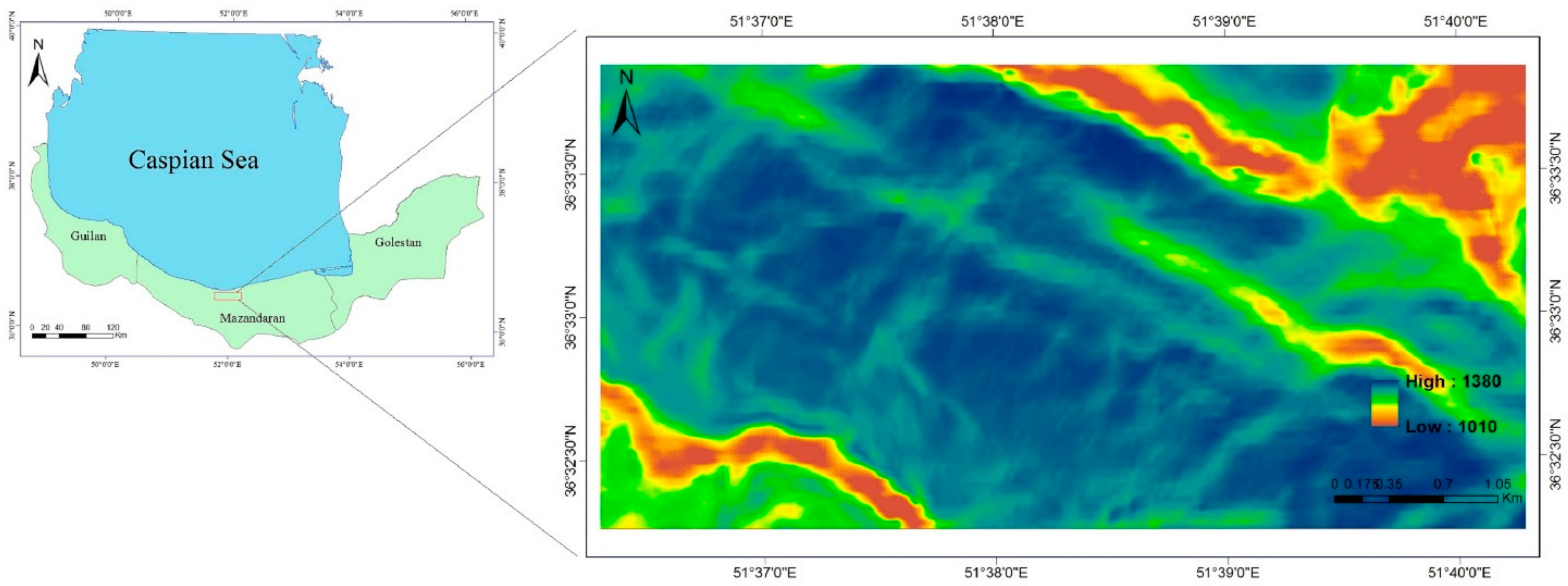
Therefore, in our research, we have used GP to study the biophysical controls on diameter-growth of Fagus orientalis in northern Iran. To this end, we have developed numerical surfaces describing the physical (abiotic) environment for a high-elevation oriental beech-dominated forest near to the Caspian Sea in northern Iran. Spatial patterns in beech development (i.e., mean DBH increment) during a nine-year growing period are related to (i) point-extractions of surfaces of growing-season-cumulated potential solar radiation (MJ m−2) obtained by computer, topographic wetness index (TWI, representing soil water and, to some extent, soil nutrient distribution), air temperature (°C), and wind velocity (ms−1) founded on principles of computational fluid dynamics (CFD), and (ii) associated field measurements of plot basal area (BA, m2 ha−1) and normalised initial mean tree DBH in individual research plots (based on 2003 data) using genetic programming.

2. Materials and Methods

2.1. Study Area and Plot Network

Hyrcanian (Caspian) forest which is located in northern Iran has an area of about 1.85 million ha. (Figure 1). This region is highly productive due to its humid, temperate climate and fertile soils. However, large portions of lowlands in this forest are void of forest cover due to the excessive human settlement, as early as 1100 AD, in these regions [5].
Figure 1 shows the Hyrcanian forest in northern Iran central to the current beech-growth study. The Caspian Sea is located in north-northeast of the study area.
Beech forests in this region contain Acer velutinum, Alnus subcordata, Carpinus betulus, and various other species of trees and shrubs. With the exception of the presence of Taxus bacata and Cupressus at certain sites, most forests in this region are broadleaved [19]. The harvesting method currently employed in the region is close-to-nature silviculture (a management system based on small-scale interference and group selection). This forest-management approach is best suited for establishing and maintaining mixed forests [20] and permanent forest cover [21]; it is similar to the approach practiced in North America.
Kheyrud forest was the experimental forest, an 80-km2 unmanaged section of the greater Hyrcanian forest, located approximately 7 km east of the port city of Noushahr (36° 39′ N, 51° 30′ E; datum WGS84). The Gorazbon section, in which the plot network is located, is one of eight sections of the Kheyrud forest (Figure 1). The northern, lower boundary of this section is situated at an elevation of 1010 m above mean sea level AMSL, while the highest elevation of this section is at 1380 m AMSL. About 80 tree species and 50 shrub species exist in the Kheyrud forest [22]. Based on the climate data from 1977–2005, the average annual precipitation in this area is 1397 mm (758 mm during the growing season) with October being the wettest (258 mm) and July the driest (33 mm) month. The average annual temperature is 15.5 °C, with February being the coldest (7.4 °C) and August the warmest (25.4 °C) month. The mean annual evaporation at the city of Noushahr is approximately 1031 mm, with the average monthly evaporation being the highest in August (155 mm) and the lowest in January (26 mm) [3].
A rectangular grid (150 m × 200 m) was employed to design the plot network in the Gorazbon section and it consisted of 258 fixed-area plots of 0.1 ha each. In 2003 and 2012, all living stems greater than 7 cm in DBH were measured using a caliper. The overall plot BA was the total basal area of all species. The total number of plots containing oriental beech was 176.
In this study, we estimated the distribution of BA and DBH outside the plots by kriging which is an interpolation method based on the spatial correlation of data points in which one can obtain the value of a quantity at points with known coordinates using the same quantity elsewhere with the specified coordinates [23,24]. In fact, this method applies for irregular data distributed, which produces new data with minimum variance and is estimated in two general ways: Ordinary and universal [25].

2.2. Data Used

2.2.1. Computational Fluid Dynamics

Computational fluid dynamics (CFD) is a numerical modelling technique which allows the use of fluid motion equations to solve three-dimensional and time dependent complex problems. This technique can be used as a precise tool for measuring various environmental variables in a virtual environment. The nature of this method is suitable for most parametric studies or flow-physics research. Additionally, it is used in many fields of engineering such as agriculture and forestry [26].

2.2.2. Development of Abiotic Surface

The key factor of spatial calculation of abiotic surfaces is the digital elevation model (DEM) describing part of the experimental forest-landscape terrain involving the plot network. The DEM of the study area was obtained from the advanced space borne thermal emission and reflection radiometer (ASTER) 30-m resolution Global Digital Elevation Model v. 2 (http://asterweb.jpl.nasa.gov/gdem.asp, last accessed in November, 2016). Descriptions of individual abiotic (environmental) surfaces and their derivations follow below.
Figure 2A shows growing-season distributions of abiotic variables; different colours indicate the spatially varying intensity of the variable. Distributions include (A) cumulated incident solar radiation (MJ m-2), (B) near-surface air temperature (°C), (C) topographic wetness index (unitless), and (D) wind velocity (m s−1). The network of forest plots is located at the centre of each image, given for reference. Intensity of solar radiation varies from dark purple (low intensity; ~1700 MJ m−2) to lighter purples (high intensity; ~4500 MJ m−2). Air temperature decreases from mean sea level (~21.1 °C) to ~2200 m AMSL as a function of environmental lapse rate (i.e., 6.5 °C km−1). The greens in (C) represent wetter areas of the landscape, either as a result of the presence of wetlands, pools, or low-ordered streams. The blues represent dryer areas. The cyan and yellows in (D) represent areas of the landscape that experience low (~0.1 m s−1) and high wind velocities (~13 m s−1), respectively.

2.2.3. Solar Radiation

Tree growth and tree distribution are altered differently for different species by solar radiation. Shade-intolerant species such as red maple (Acer rubrum L.) and white birch (Betula papyrifera Marsh.) exploit low light levels less efficiently than shade-tolerant species like sugar maple (Acer saccharum Marsh.) and American beech (Fagus grandifolia Ehrh.) [27]. Due to maximizing light interception and minimizing respiration, shade-intolerant species tend to show lower growing potentials in regions naturally low in sunlight [28,29]. Oriental beech seedlings and saplings alter their sensitivity to incident solar radiation as they mature [30].
In this study, incoming solar radiation was evaluated as a function of (i) DEM-based calculations of slope, view factor, terrain configuration factors, aspect, and horizon angle; (ii) solar-illumination angles and sun-earth geometry; and (iii) solar-flux calculations at the top of the atmosphere, based on calculations from the LanDSET (landscape distribution of soil moisture, energy and temperature) model of Bourque et al. [6] (Figure 2A) Sunlight penetrating the top of the earth’s atmosphere is divided into direct and diffused components, as a function of the angle of incidence. Both of these radiation components react differently as they pass through the atmosphere and come into contact with the underlying terrain [28]. Many geographic information systems (e.g., ArcGIS, and the Environmental Systems Research Institute ESRI GIS product) contain subroutines to spatially calculate cloud-free and potential solar radiation.

2.2.4. Seasonal Air Temperature

Plant growth often correlates with indices of annual heat inputs, since increasing temperature induces an increase in plant metabolism and growth [31]. In the present study, we have used the mean air temperature during the growing-season as an index of growing-period heat input.
The seasonal distribution of air temperature is based on decreasing the growing-season mean air temperature (April–October) at Noushahr station (i.e., 21.2 °C; based on data collected between 1977 and 2005) as a function of elevation and an assumed mean environmental lapse rate of 6.5°C km-1 over land (Figure 2B). The environmental lapse rate is an indicator of the long-term average air temperature gradient, which is inversely proportional to elevation. In general, a lapse rate is the negative of the rate of temperature change with altitude change, [3,32].

2.2.5. Topographic Wetness Index

Tree species differ regarding soil water requirements and tolerances. Since soil characteristics information and precipitation patterns were not available, we represented the soil water distribution solely as a function of TWI. Topographic wetness index (TWI) is a common and useful tool for describing the basin’s humidity conditions, which is usually used in determining the topographic control in hydrological processes and is calculated as follows:
TWI= Ln (As/tanβ)
where As is the surface area of the basin that is based on the cumulative upstream area and β is the local slope. This index has been used in many studies [33] to estimate the physical, hydrological, and chemical properties of soil, and also for biological descriptions, plant distributions, forest habitat and etc. [34]. (Figure 2C). This is reasonable that precipitation and thus soil water are spatially distributed by topography. Thus, spatial TWI data can be developed from DEM height data [35]. Topographic wetness index assumes steady-state (long-term) conditions and uniform soil-water infiltration and transmissivity. Several methods can be used to calculate TWI In the present study, the upslope contribution area in TWI was calculated by the mass-flux method in RiverTools.

2.2.6. Wind

Wind velocity is another important abiotic variable which affects plant production. Wind velocities impact on plants can be positive and negative, in terms of both physiological and physical properties. At low wind velocities, the transfer of carbon dioxide gas to the plant cells is prevented due to the large boundary-layer resistances between the surrounding air and leaf surface, which lowers the ability of the plant to grow [36]. At high wind velocities, the growing pattern of plants is distorted by exerting a constant bending-pressure on all parts of the plant, especially the main stem, which leads to breakage and possibly permanent deformation. High wind velocities also contribute to the rapid perspiration of the plants (i.e., losing water content to the atmosphere) and trigger closure of the stomata to prevent desiccation, which reduces the uptake of carbon dioxide. Optimal growing conditions have been observed regarding to wind velocity to occur somewhere in between these two extremes [37]. (Figure 2D).
Given the complexity associated with the calculation of wind velocity and direction, this variable has been rarely used in plant growth studies. In this study, a CFD simulator was employed to model wind flow over complex terrain based on the DEM.
The effects of atmospheric turbulence and thermal processes were included in this model, which solves the full 3-dimensional Navier–Stokes equations [5]. The model calculations were based on a boundary-fitted coordinate system, with initial conditions specified by (i) mean surface air temperature of the growing season (same as before) and wind velocity and direction (i.e., 1.7 m s−1 and 333° from true North) based on the Noushahr station climate records (1977–2005), and (ii) an assumed wind velocity at 500 m from ground level (i.e., 6 m s−1). The atmospheric temperature gradient was assumed to be 9.86 °C km−1), which is common for windy and cloudy conditions during the day [3].

3. The Principles of the GP

As mentioned before, the GP technique derives from the theory of “survival of the fittest” and biological evolution. The most important components of GP are firstly the functional and terminal sets. The first set includes any mathematical function (the choice of function determines the degree of complexity). The latter set contains variables (program inputs), numerical constants, and random input. Secondly, the GA involves fitness function and different operators, such as crossover, mutation, reproduction, and so on. Different fitness functions that determine the fitness of an objective function within a particular search space, depend on the nature of the problem. Thirdly, the GA has patterns of learning. Terminals and mathematical functions are combined to create a computer-based tree structure model. The tree structure consists of a node in each root, and branches, that are expelled from each function and end in a terminal. 
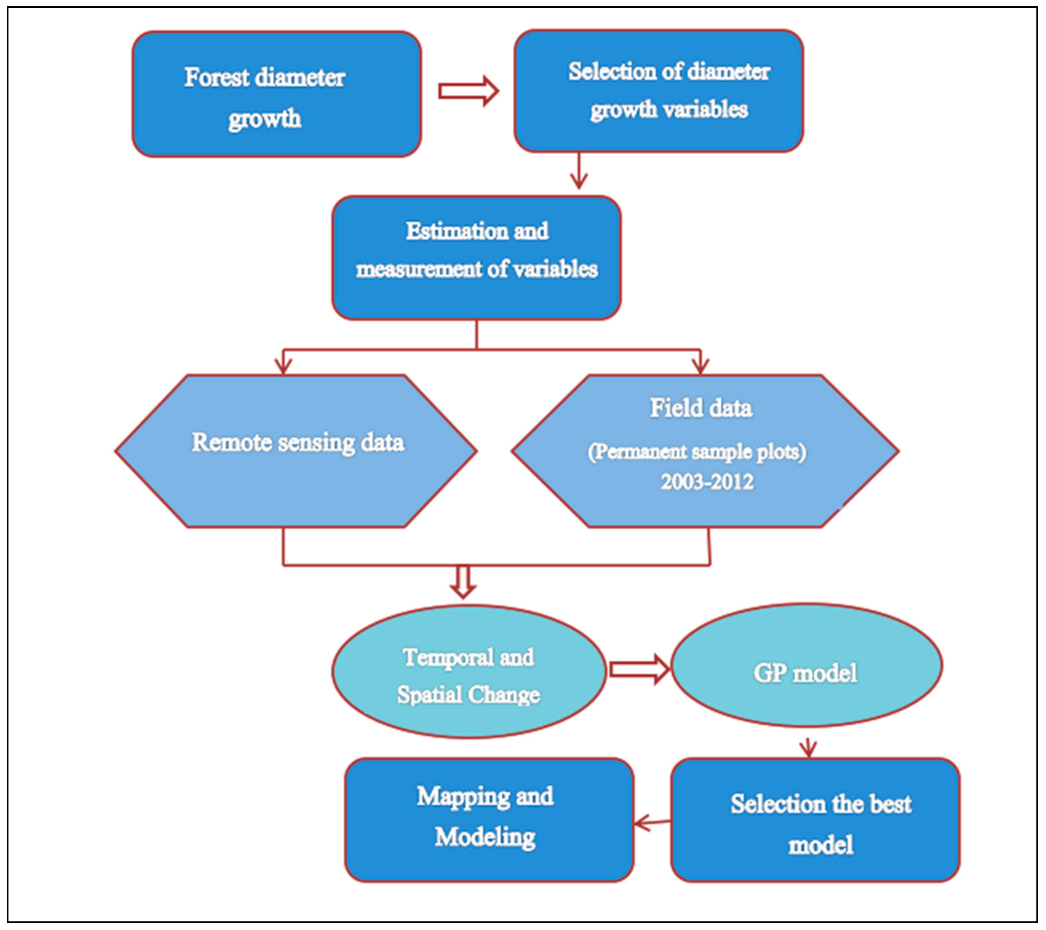
Figure 3 gives a general workflow of the GP method.
In general, to solve a problem, the GA forms a basic population (each individual in the GP plays a possible solution to solve the problem and has a fitness) which is created randomly from the combination of functions and terminals, as previously described. Then a new population (computer program) is formed based on the fitting theory of choice and the fitness score, which is actually generated through reproduction, mutation and crossover. In the next step, each individual is evaluated for the solution of the problem. The best individuals are selected and are used to produce a new population. This process is repeated until the stopping criterion is met.
There are several ways to present a computer program in GP such as gene expression programming (GEP), aka GP variants, monolithic GP and linear GP (LGP) [12,38,39].

Proposed Genetic Programming for the Study of Biophysical Controls on Diameter-growth of Fagus orientalis

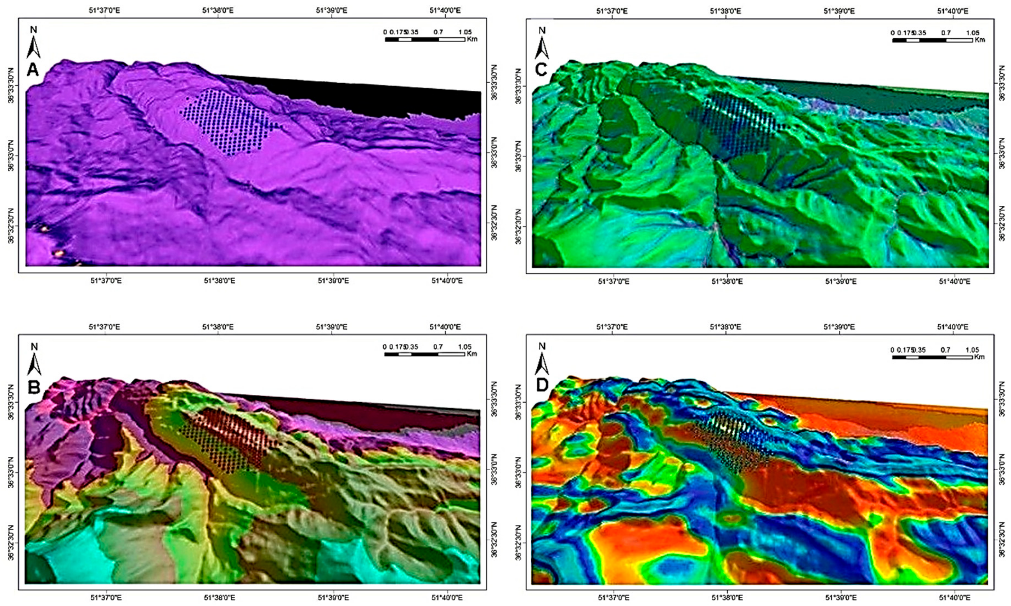
Abiotic conditions (
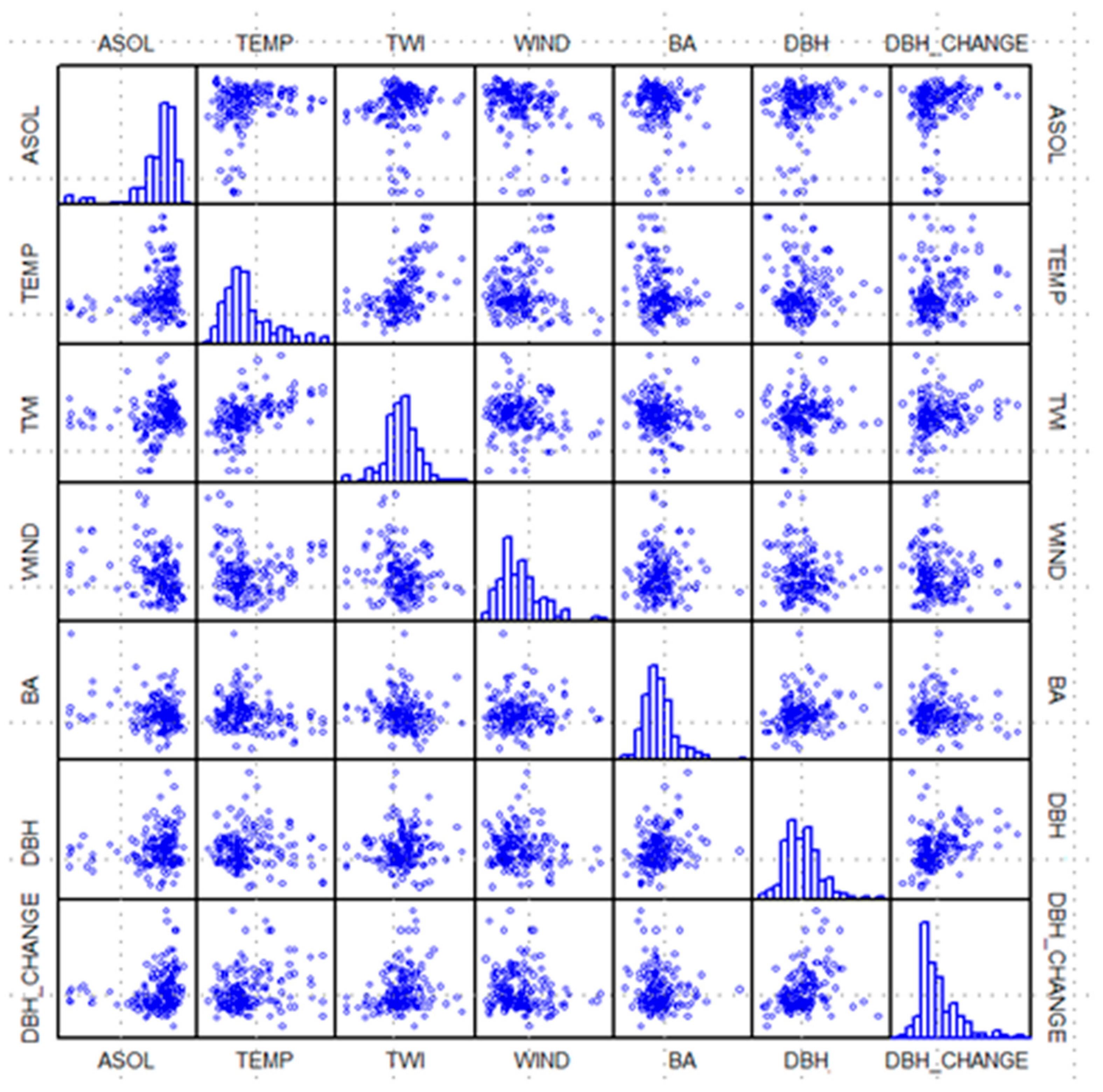
Figure 2) at forest-plot locations were averaged within each 0.1-ha plot. For every plot containing beech (in total 176), plot records comprised the mean values of all abiotic and biotic variables (six predictors) and 9-year DBH increment (predicted variable). Comparative scatter plots of plot values for the seven variables are provided in Figure 4. Four abiotic (ASOL = average growing-season-cumulated incident solar radiation, TEMP = air temperature, TWI, and WIND) and two biotic independent variables (BA and DBH), and one dependent variable (DBH_CHANGE = 9-year mean DBH increment). Histograms along the diagonal, give the distribution of values for each of the seven variables.
The initial DBH (2003) was normalised by dividing its value by the maximum diameter (i.e., DBHmax) oriental beech is known to grow in the Hyrcanian forest (~200 cm) ecosystem [40] and subtracting the quotient from one, i.e., 1.0-DBH/DBHmax; hereafter, DBH-factor. The DBH-factor describes the influence of DBH on 9-year DBH increment as diameter approaches DBHmax.
Basal area is included in the list of independent variables to incorporate the effects of inner-plot tree competition on mean DBH increment [41]. 
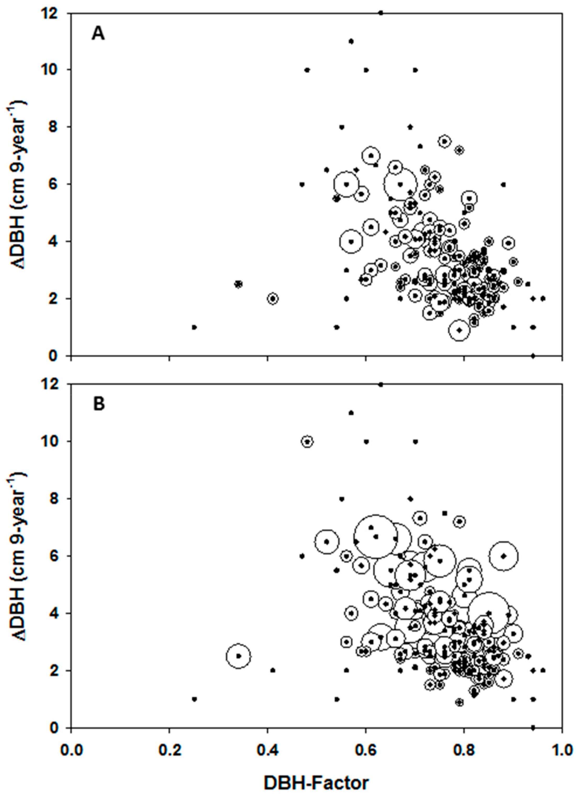
Figure 5 displays plot-level DBH increment (i.e., DBH, y-axes) as a function of the DBH-factor (x-axes). The same data is displayed spatially over calculations of habitat suitability index (HSI) for oriental beech (Figure 6), according to the procedures given by Bourque et al. [6] and Baah–Acheamfour et al. [42]. The index only accounts for variation in abiotic conditions and not for inter- and intra-species competition (i.e., BA) and tree growth potential (DBH-factor).
Calculation of HSI was revised in this study to use mean air temperature and TWI instead of growing degree-days (GDD) and soil water content, as was originally done in Bourque et al. [6] and Baah-Acheamfour et al. [42]. Also, a new element was added to the calculation of HSI to account for the effect of wind on species performance and distribution. The species response to wind was modelled as a beta function (6) with the minimum and maximum wind velocity at zero and 14 m s−1, giving zero response (0.0), and 2.4 m s−1, optimal response (1.0). Threshold values for the environmental-response function for air temperature, TWI, and wind velocity were based on the upper envelop created by the distribution of abiotic values (x-axis) to DBH increment (y-axis) plotted in Figure 4; in particular, the graphs along the bottom row. Response to solar radiation was handled in the same manner as given by Bourque et al. [6]. Relating DBH increment to the abiotic and biotic variables is achieved with the benefit of GP. As the number of plots was limited, the dataset was partitioned into two parts: 144 plots selected randomly for training and the remaining 32 plots for validating the GP-generated code. A larger subdivision of the dataset was needed for training in order to capture the greatest amount of spatial variability associated with differences in elevation. Validation was done to ensure that the code created with GP had the ability to simulate mean growing conditions of oriental beech in plots not used in training.
We subsequently used the validated code to examine the impact of changing current distributions of BA and initial DBH with a spatially-uniform distribution of mean-values of BA (37.4 m2 ha−1) and DBH-factor (0.75, based on the average of current plot values) on the 9-year mean increment in DBH across the study stand, as an illustration of model application. A uniform DBH-factor distribution of 0.75 implies that all beech trees in the area have an effective DBH of 50.6 cm or 25% of DBHmax. Development of the current DBH-increment surfaces requires the plot-level BA and initial DBH to be interpolated at the appropriate spatial resolutions (i.e., 30 m) for input into the –spatial diameter-increment model. The nine-year mean increment in oriental beech (from 2003 to 2012) as a function of DBH-factor, i.e., 1.0-DBH/DBHmax; the DBH-factor is calculated from 2003 DBH as seen in Figure 5. Standard deviations in DBH increment were normalised as a function of largest mean DBH increment (i.e., 12 cm 9-year-1) in order that related bubbles fit on the graph (B). Closed circles in both graphs without bubbles represent plots with a single beech tree.
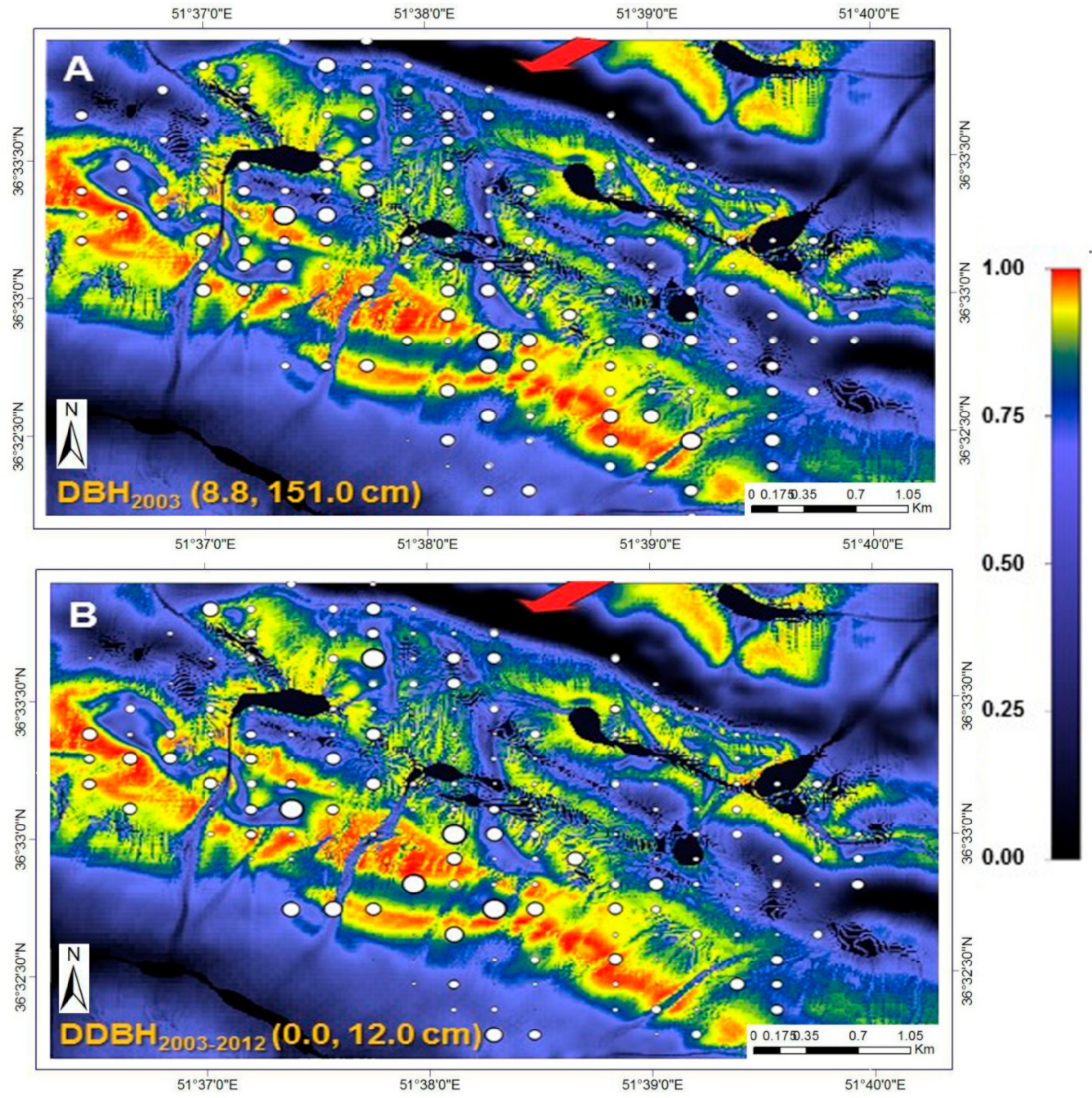
The size of the circles in Figure 6 varies according to actual DBH (2003) and mean DBH increment; their ranges are specified at the bottom left of their respective illustrations. Background colours are calculated habitat suitability index (HSI; see colour bar). Black areas in the high-elevation portion of the study area (top-to-central portion of the plot network) are associated with landscape depressions that regularly fill with water. The red arrows indicate the prevailing wind direction on the windward and high-elevation ridge of the study area, modelled with the CFD wind-flow simulator [43].

4. Results

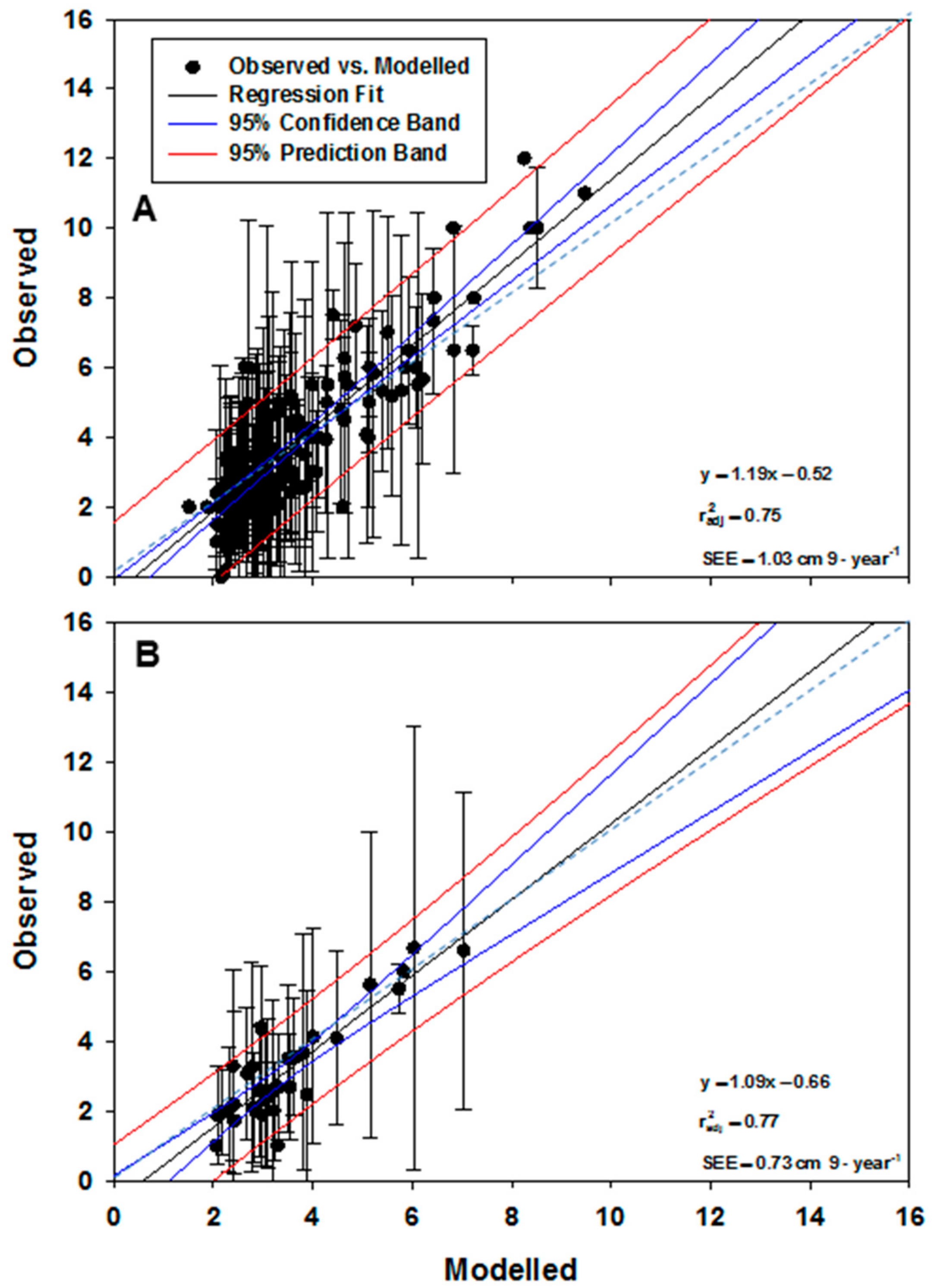
Figure 7 illustrates the performance of the GP-generated model using the training (Figure 7A) and validation (Figure 7B) data sets. The overall degree of explained variance was 75% in the training data set and 77% in the validation data set. Some under prediction is evident during training; plotted modelled vs. averaged growth summaries gave a regression slope > 1.0 and a standard error of estimate (SEE) = 1.03 cm 9-year−1 (Figure 7A). Under prediction was less apparent during validation; slope = 1.09 compared to 1.19 for training and SEE=0.73 cm 9-year−1. Overall mean offset for both cases was < 0.7 cm 9-year−1. Given the disproportionate amount of variation in individual-tree DBH increment (for both training and validation datasets) suggests that, although not perfect, the GP-generated code is most likely the best possible explanation of mean DBH increment in oriental beech, notwithstanding the possible imprecision in abiotic surfaces.
In Figure 7, in both instances, plot variation in actual DBH increment is specified as vertical error bars (first standard deviation). The closed circles without bars represent plots with a single beech tree. The diagonal dashed line (in dark cyan) specifies a 1:1 data correspondence. Regression statistics apply to the lines fitted to the average DBH increment in individual plots; SEE is the standard error of estimate. The dark blue lines give the 95% confidence band and the red lines, the 95% prediction band.
Multivariate analysis with GP reveals that averaged DBH increment over the 9-year period was potentially equally controlled by the four abiotic factors, together contributing to about 50.8% of the total control, and the two biotic factors (49.2%; Table 1). The DBH-factor (potential tree growth factor) provided the greatest influence on plot-level tree growth (32.3%), followed by topography and the re-distribution of soil water (via TWI; 19.5%), and plot BA (16.9%). On average, long-term solar radiation together with wind velocity likely controlled 20.1% of plot-level mean growth in oriental beech (Table 1). DBHmax was set equal to the maximum allowable DBH (i.e., 200 cm) for oriental beech, based on existing data and literature [5,44].
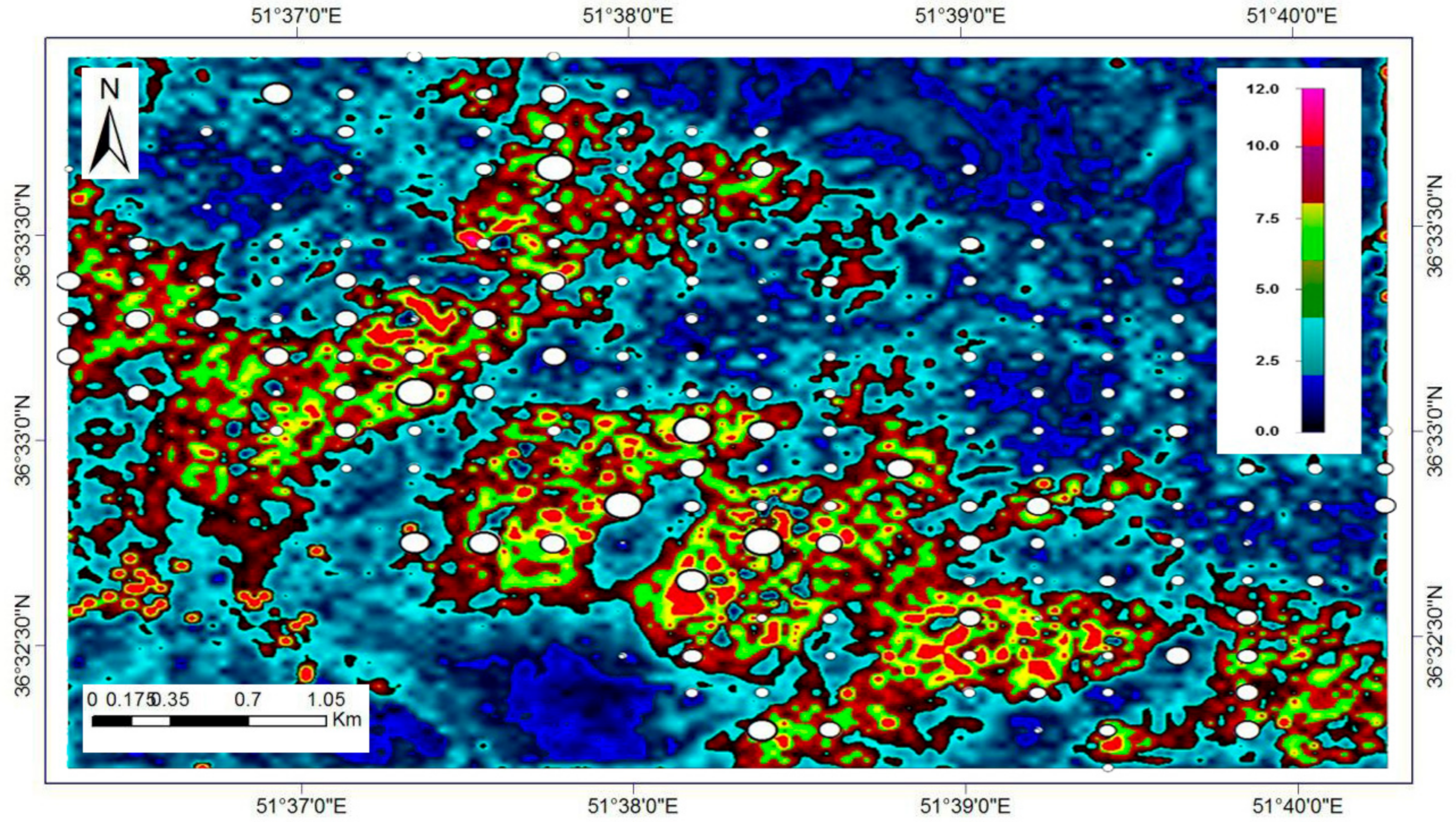
Figure 8 describes the growing conditions of oriental beech for the entire study area. The colours express variation in beech DBH increment over the nine-year period. Superimposed are the actual mean growing conditions for individual plots. Generally, beech plots in high wind velocity (>9 m s−1) and high TWI (<−4.0, indicative of high soil moisture; dark blue areas) tended to exhibit low growth (≤1.3 cm 9-year−1). The least amount of growth occurred in plots found in landscape depressions (Figure 6) that regularly fill with water during the spring-melt and winter seasons. Excessive soil moisture for extended periods contributes to unfavourable conditions for the growth of beech. The adverse effects of “high wind velocities” and “soil moisture” (TWI) on mean tree growth can be demonstrated both in terms of the initial mean DBH (for those plots in high wind velocity and “soil moisture” areas) and 9-year mean DBH increment (Figure 6 and Figure 8). The best growth (>10.0 cm year−1) is shown to occur where all abiotic and biotic attributes (low BA and medium DBH) are retained in the best (red to pink colours). Plots with high BA (high intra- and inter-species competition) and larger trees (low growing potential and, thus, low DBH-factor) are expected to grow more slowly, irrespective of the prevailing site environmental (abiotic) conditions.
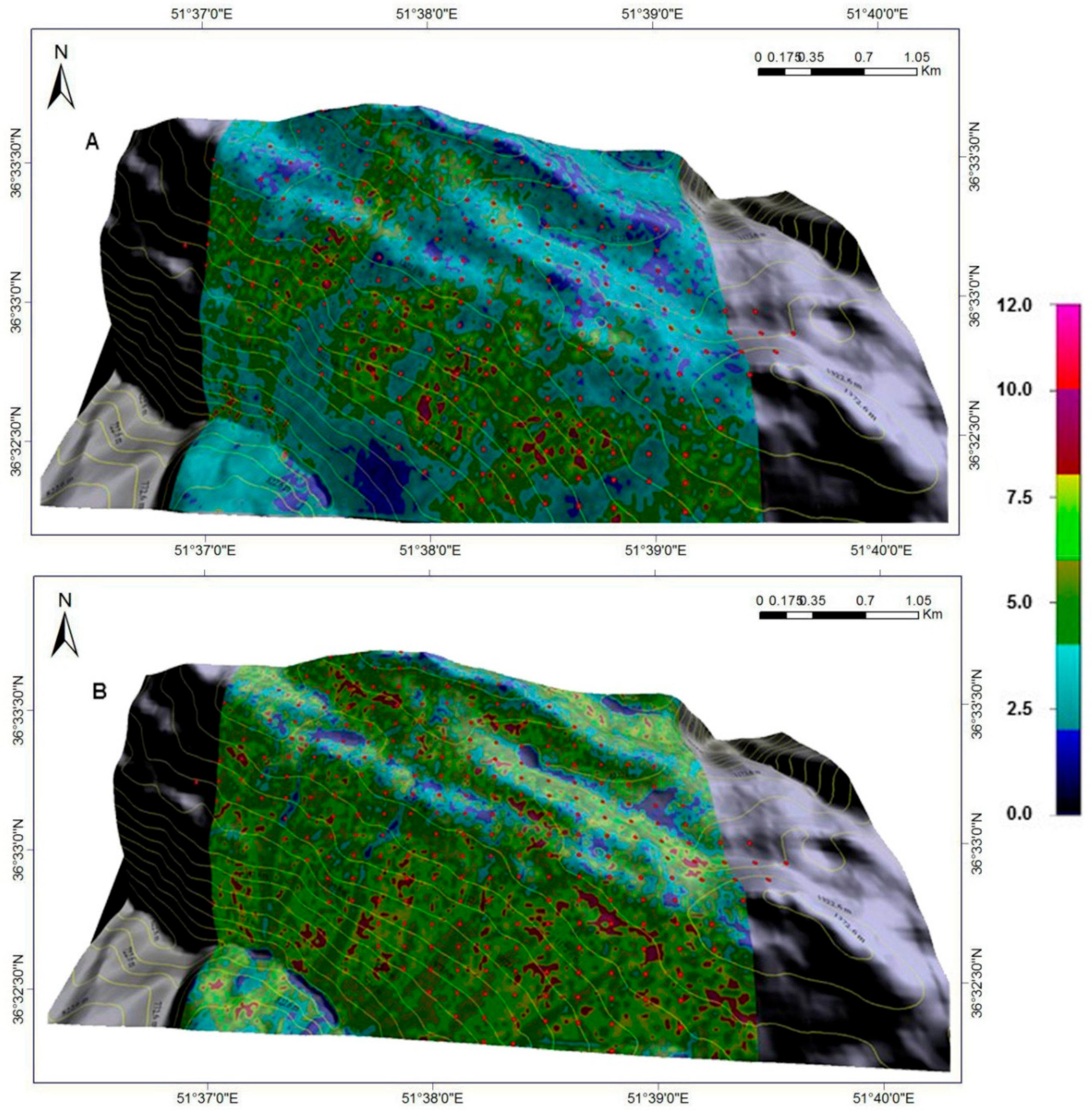
Figure 9 provides a comparison of beech DBH increment over the 9-year period for current and assumed spatially-uniform BA (37.4 m2 ha−1) and initial DBH (50.6 cm, or 0.75 in its normalised form) for similar abiotic conditions. By reducing BA and initial DBH (increasing tree-growing potential), the effect on the 9-year DBH increment increased throughout the study area (Figure 9B), except in areas predisposed to high wind velocities (windward, high-elevation side of the plot network; Figure 2D and Figure 5), low incident radiation, and elevated soil moisture (black areas in the top-to-central portion of the plot network; Figure 6). In general, management of these forests, by reducing BA and DBH by thinning and/or selective harvesting, can have a pronounced positive effect on the distribution of DBH in the future (Figure 9B).

5. Discussion

In this paper, we used an artificial intelligence method, i.e., GP, to study the factors affecting diameter growth. The advantage of this method in comparison with other empirical methods is that GP is highly flexible with the ability to solve many management problems associated with forest management. Using this method, a modeller can design a flexible framework to analyse the problem efficiently [12,38]. Our results demonstrated the capability of GP to study the biophysical controls on diameter-growth of Fagus orientalis in northern Iran and to identify the predictors (WIND, TWI, BAL, diameter, and temperature) that contribute the most to growth rate. This can be attributed to the nature of GP that can handle manifold information of environmental variables to significantly improve the quality of the results. In contrast to MLR and other statistical-based methods, GP and other machine learning methods extract knowledge directly from data without any pre-defined assumptions of the phenomenon being [15].
Verification of computer-generated surfaces at enhanced spatial resolution needs a large amount of field data, which is rarely conducted (Figure 2). Satellite data can be employed for verifying some of these images (especially air temperature and incident solar radiation), but this is not feasible at the utilized spatiotemporal resolution (i.e., at 30-m resolution and over the long term) without extensively processing the data from the images. TWI and wind velocity are difficult to ascertain without broad assumptions being made, since they are difficult to measure at a small and consistent scale. TWI can be verified by satellite-derived soil water distribution, however, the forest canopy obscures the ground surface from a satellite view. Even with these necessary assumptions, the physical conditions of the Gorazbon section are meaningfully represented by our modelled abiotic surfaces. Since abiotic data are rarely collected at the plot level, plot-level abiotic conditions estimated from numerically-derived surfaces can serve as reasonable alternatives in the prediction of beech growth over both space and time. Computational methods used in the generation of these data at appropriate resolutions decreased the need to collect this information in the field and, thus, helped curb costs. Numerical estimates of abiotic conditions at the plot level (based on 30-m resolution calculations), along with two simple forest-state descriptors, are shown to explain a significant portion of the plot-level variability (>75%) in mean DBH increment (in the training and validation data; Figure 4) after 65 h of continuous searching for an optimal solution with GP. Conceivably, the results could have been improved with the application of more advanced GIS-based operations [45] and LiDAR (light detection and ranging)-based DEMs at sub-metre resolution in the production of plot-level estimates of the physical (abiotic) environment. As beech growth is influenced by the actual state of the forest, i.e., crowding and level of competition among member trees and their dimensions, the method requires that plot-level BA and DBH distribution be made available for input. This information is routinely collected by most forest-monitoring networks. In the absence of BA and DBH measurements, there are LiDAR-based and data-processing techniques that can be used to generate the required information at enhanced spatial resolutions [46,47,48]. The machine learning methods have been proven to be effective methods for different types of environmental research. For example, Vafaei et al. [18] showed the ability of random forest (RF), support vector regression (SVR), MPL neural nets and Gaussian process (GP) to estimate the aboveground biomass in the Hyrcanian forest of Iran. In another study, Castelli et al. [49] used the GP for the prediction of forest fire and showed that GP can significantly outperformed the other methods and has a higher ability to predict than other machine learning methods.
For this study, we estimated the distribution of BA and DBH outside the plots by kriging. Accuracy of interpolation with kriging and with other single-input spatial interpolators is widely known to decline with increased distance from the input-data source (in this case, the plot network). We use kriging here solely to illustrate the computational attributes of the modelling system. More precise estimates of outer-plot BA and DBH would have helped to reduce uncertainty in calculations outside the plot network (Figure 2B).
While this model was created for a certain area at a specific time, it could be used for greater areas and time scales by scaling up to entire landscapes. With data from multiple measurement periods (e.g., every 5 years over the lifetime of forests) and revised model formulation by means of GP, this same process could be used to evaluate the state of forests at multiple times throughout the normal lifetime of forests, including after catastrophic disturbance [3,5]. If the data from forest plots are combined with the computer-generated abiotic variable results that are obtained from evolutionary algorithms, our assessment and predictive capability of forest growth in variable landscapes will become advanced at medium spatial resolutions (<100 m). Moreover, the effects of climate change on forest development is quantifiable, if the output of existing global or regional climate models can be used to quantify the change to abiotic variables, since the growth of forests and abiotic conditions are connected. Climate is one of the major forces shaping the forest landscape dynamics in terrestrial forest ecosystems. Responses of tree growth to climate factors were spatially dependent because of spatial variability (e.g., topographic heterogeneity, environmental site conditions, and species interactions) [50]. Moreover, increased frequency and intensity of environmental perturbations could cause physiological disorders, resulting in large-scale increases of die-off events [49]. Decreased growth rates in plots are frequently seen in areas of the landscape under higher wind velocities and elevated soil moisture (TWI) content, especially in large, frequently saturated depressions on the landscape.
The interactions between wind and trees and forest stands occur at a broad range of temporal and spatial scales. Wind direction and velocity can have both positive and negative impacts on plant growth and performance, both physiologically and mechanically. At low wind speeds, a thick boundary-layer between the leaf surface and surrounding air reduce the water vapor and carbon dioxide fluxes to and from inside of the leaf, resulting in growth in plants to proceed at reduced values [51]. At higher wind speeds and strong wind conditions, however, developmental patterns of the plants could be affected in different ways such as shoot (stem, branches, leaves, crowns, twigs, etc.) breakage, uprooting of whole tress, triggering closure of stomatal pores, reducing the absorption of carbon dioxide, consequently, diminishing plant growth [51].
Presence and dominance of oriental beech in the wetter areas of the forest are compatible with the preference of this species for such conditions [5]. In forests, incoming solar radiation is fundamental for different physical, physiological and biochemical processes (e.g., air and soil heating, carbon cycling, photosynthesis, growth and development, evapotranspiration, winds, temperature regimes and snow melt) at the earth’s surface due to its key role in energy and water balance [52]. Notwithstanding this important role, solar radiation has received comparatively less attention with regards to other abiotic environmental factors such as wind, temperature and precipitation, mostly due to the difficulties of measuring solar radiation. Nevertheless, it has been acknowledged that differences exist among the stands in terms of their tolerance/sensitivity degrees to shade. While shade-intolerant trees are typically pioneers in terrestrial ecosystems, shade-tolerant species of trees (e.g., oriental beech) establish later in ecosystem development since they can grow under the dense stand canopies and/or at least survive until a gap formation. Favorable light regime variability is fundamental for tree growth, establishment and productivity; therefore, optimizing light distribution for seedlings and saplings is an important aspect of forest management practices.
Understanding forest ecosystems is important given current forest-management needs and climate change. Studies such as this one are necessary to sustaining natural resources.

6. Conclusions

The current manuscript provides a semi-empirical approach based on GP for analyzing biophysical controls on diameter increment of oriental beech in a subsection of the Hyrcanian forest in northern Iran. It relates diameter increment in oriental beech to plot-values of computer-generated abiotic and field-based biotic variables, explaining >75% of the variation in plot-level DBH increment. Multivariate analysis with GP showed that the control on beech diameter increment is most likely evenly split between abiotic and biotic variables, with the greatest control attributed to the initial (2003) DBH or tree-growing potential. Large trees grew at a lower rate, irrespective of other site variables. Also, intra- and inter-species competition had some control (16.9%) on the rate beech can grow. Reduced growth rates in plots were usually seen in areas with high wind velocities (e.g., the windward and high-elevation ridge of the study area), as well as in elevated soil moisture (TWI) areas (i.e., large, frequently saturated depressions in the landscape). Management of biotic factors with favorable expectations can have a positive quantifiable impact on DBH-distribution in the future. Improved calculations are possible with the incorporation of enhanced LiDAR-based DEMs and landscape-assessments of forest state. The GP modelling system provides forest managers with an initial limited tool to evaluate different management strategies on the state of the forest over a small portion of the Hyrcanian forest and over a specified time interval. The methodology can be used in support of close-to-nature silvicultural practices by providing forest managers a means to describe the short-term functional response of oriental beech, particularly with respect to variable physiography. The current modelling system is sufficiently general to be employed for the analyzing of growth patterns of species of trees not included in this study and forest-development patterns in forested areas around the world.

Author Contributions

M.B. conceived and designed the experiments; M.B. and D.T.B. performed the experiments and analyzed the data; P.T. and R.Z. contributed reagents/materials/analysis tools; M.B., D.T.B, P.T.N. and R.Z. wrote the paper.

Funding

This research received no external funding.

Acknowledgments

We are particularly grateful to: (i) Charles P.-A. Bourque of the Faculty of Forestry and Environmental Management, University of New Brunswick, Canada, for his comprehensive examination of the paper with respect to both its scientific content and presentation and help to authors in the generation of abiotic surfaces; (ii) the Natural Resources Faculty, University of Tehran, Karaj, Iran, for our use of the Kheyrud Experimental Forest and for logistical and financial support to MB; (iii) We acknowledge the USA National Aeronautics and Space Administration for providing ASTER GDEM v. 2 and Landsat-8 data free of charge. We also thank anonymous reviewers who provided many helpful comments and suggestions for improving this manuscript.

Conflicts of Interest

The authors declare no conflict of interest.

References

  1. Ashraf, M.I.; Zhao, Z.; Bourque, C.P.A.; MacLean, D.A.; Meng, F.R. Integrating biophysical controls in forest growth and yield predictions with artificial intelligence technology. Can. J. For. Res. 2013, 43, 1162–1171. [Google Scholar] [CrossRef]
  2. Bohora, S.; Cao, Q. Prediction of tree diameter growth using quantile regression and mixed-effects models. For. Ecol. Manag. 2014, 319, 62–66. [Google Scholar] [CrossRef]
  3. Bourque, C.P.A.; Bayat, M. Landscape Variation in Tree Species Richness in Northern Iran Forests. PLoS ONE 2015, 10, e0121172. [Google Scholar] [CrossRef] [PubMed]
  4. McPherson, E.; Peper, P. Urban Tree Growth Modeling. Arboric. Urban For. 2012, 38, 172–180. [Google Scholar]
  5. Bourque, C.P.A.; Bayat, M.; Zhang, C. An assessment of height–diameter growth variation in an unmanaged Fagus orientalis-dominated forest. Eur. J. For. Res. 2019, 138, 607–621. [Google Scholar] [CrossRef]
  6. Bourque, C.P.A.; Meng, F.R.; Gullison, J.J.; Bridgland, J. Biophysical and potential vegetation growth surfaces for a small watershed in northern Cape Breton Island, Nova Scotia, Canada. Can. J. For. Res. 2000, 30, 1179–1195. [Google Scholar] [CrossRef]
  7. Liu, Z.; Jianga, F.; Zhua, Y.; Li, F.; Jin, G. Spatial heterogeneity of leaf area index in a temperate old-growth forest: Spatial autocorrelation dominates over biotic and abiotic factors. Sci. Total Environ. 2018, 634, 287–295. [Google Scholar] [CrossRef] [PubMed]
  8. Ma, P.; Hana, X.; Lina, Y.; Moore, J.; Guo, Y.; Yue, M. Exploring the relative importance of biotic and abiotic factors that alter the self-thinning rule: Insights from individual-based modelling and machinelearning. Ecol. Model. 2019, 397, 16–24. [Google Scholar] [CrossRef]
  9. Byun, J.G.; Lee, W.K.; Kim, M.; Kwak, D.A.; Kwak, H.; Park, T.; Byun, W.H.; Son, Y.; Choi, J.K.; Lee, Y.J.; et al. Radial growth response of Pinus densiflora and Quercus spp. to topographic and climatic factors in South Korea. J. Plant Ecol. 2013, 6, 380–932. [Google Scholar] [CrossRef]
  10. Lawrencea, A.; Escobedoa, F.; Staudhammera, C.H.; Zipperer, W. Analyzing growth and mortality in a subtropical urban forest ecosystem. Landsc. Urban Plan. 2012, 104, 85–94. [Google Scholar] [CrossRef]
  11. Silva, S.; Vanneschi, L.; Cabral, A.; Vasconcelos, M. A semi-supervised Genetic Programming method for dealing with noisy labels and hidden overfitting. Swarm Evol. Comput. 2017, 39, 323–338. [Google Scholar] [CrossRef]
  12. Mehr, A.; Nourani, V.; Kahya, E.; Hrnjica, B.; Sattar, A.; Yaseen, Z. Genetic programming in water resources engineering: A state-ofthe- art review. J. Hydrol. 2018, 566, 643–667. [Google Scholar] [CrossRef]
  13. Tran, B.; Xue, B.; Zhang, M. Genetic Programming for Multiple-Feature Construction on High-Dimensional ClassiÞcation. Pattern Recognit. 2019, 93, 404–417. [Google Scholar] [CrossRef]
  14. Langdon, W.B.; Poli, R. Foundations of Genetic Programming; Springer Science & Business Media: Berlin, Germany, 2013. [Google Scholar]
  15. Fotakis, D.; Sidiropoulos, E.; Myronidis, D.; Ioannou, K. Spatial genetic algorithm for multi-objective forest planning. For. Policy Econ. 2012, 21, 12–19. [Google Scholar] [CrossRef]
  16. Castro, R.; Soares, C.; Leite, H.; Souza, A.; Nogueira, G.; Bolzan Martins, F. Individual Growth Model for Eucalyptus Stands in Brazil Using Artificial Neural Network. Int. Sch. Res. Not. For. 2013, 2013, 1–12. [Google Scholar]
  17. Ashraf, M.; Meng, F.; Bourque, C.; MacLean, D. A Novel Modelling Approach for Predicting Forest Growth and Yield under Climate Change. PLoS ONE 2015, 10, e0132066. [Google Scholar] [CrossRef]
  18. Vafaei, S.; Soosani, J.; Adeli, K.; Fadaei, H.; Naghavi, H.; Pham, T.; Bui, D. Improving Accuracy Estimation of Forest Aboveground Biomass Based on Incorporation of ALOS-2 PALSAR-2 and Sentinel-2A Imagery and Machine Learning: A Case Study of the Hyrcanian Forest Area (Iran). Remote Sens. 2018, 10, 172. [Google Scholar] [CrossRef]
  19. Mohammadi, J.; Shataee, S. Possibility investigation of tree diversity mapping using Landsat ETM+ data in the Hyrcanian forests of Iran. Remote Sens. Environ. 2010, 114, 1504–1512. [Google Scholar] [CrossRef]
  20. Patry, C.; Kneeshaw, D.; Wyatt, S.; Grenon, F.; Messier, C. Forest ecosystem management in North America: From theory to practice. For. Chron. 2013, 89, 525–537. [Google Scholar] [CrossRef] [Green Version]
  21. Lindenmayer, D.; Franklin, J.F.; Lohmus, A.; Baker, S.C.; Bauhus, J.; Beese, W.; Brodie, A.; Kiehl, B. A major shift to the retention approach for forestry can help resolve some global forest sustainability issues. Conserv. Lett. 2012, 5, 421–431. [Google Scholar] [CrossRef] [Green Version]
  22. Bayat, M.; Pukkala, T.; Namiranian, M.; Zobeiri, M. Productivity and optimal management of the uneven-aged hardwood forests of Hyrcania. Eur. J. For. Res. 2013, 132, 851–864. [Google Scholar] [CrossRef]
  23. Oliver, M.A.; Webster, R. Kriging; a method of interpolation for geographic information system. Geogr. Inf. Syst. 2007, 4, 313–332. [Google Scholar]
  24. Zhang, T.; Xu, X.; Xu, S. Method of establishing an underwater digital elevation terrain based on kriging interpolation. Measurement 2015, 63, 287–298. [Google Scholar] [CrossRef]
  25. Gomroki, M.; Jafari, M.; Sadeghian, S.; Azizi, Z. Application of Intelligent Interpolation Methods for DTM Generation of Forest Areas Based on LiDAR Data. PFG 2017, 85, 227–241. [Google Scholar] [CrossRef]
  26. Norton, T.; Sun, D.; Grant, J.; Fallon, R.; Dodd, V. Applications of computational fluid dynamics (CFD) in the modelling and design of ventilation systems in the agricultural industry: A review. Bioresour. Technol. 2007, 98, 2386–2414. [Google Scholar] [CrossRef] [PubMed]
  27. Dong, S.H.; Davies, S.; Ashton, P.; Bunyavejchewin, S.; Supardi, M.N.; Kassim, A.; Tan, S.; Moorcroft, P. Variability in solar radiation and temperature explains observed patterns and trends in tree growth rates across four tropical forests. Proc. R. Soc. B 2012, 279, 3923–3931. [Google Scholar] [CrossRef] [PubMed]
  28. Duursma, R. Physiological ecology of forest production: Principles, processes, and models. Tree Physiol. 2011, 31, 680–681. [Google Scholar] [CrossRef]
  29. Weiskittel, A.R.; Hann, D.W.; Kershaw, J.A.; Vanclay, J.K. Forest Growth and Yield Modeling, 2nd ed.; Wiley-Blackwell: Chicester, UK, 2011. [Google Scholar]
  30. Petritan, A.; Lüpke, B.; Petritan, I. Effects of shade on growth and mortality of maple (Acer pseudoplatanus), ash (Fraxinus excelsior) and beech (Fagus sylvatica) saplings. Forestry 2007, 80, 397–412. [Google Scholar] [CrossRef]
  31. Wahid, A.; Gelani, S.; Ashraf, M.; Foolad, M.R. Heat tolerance in plants: An overview. Environ. Exp. Bot. 2007, 61, 199–223. [Google Scholar] [CrossRef]
  32. Hatfield, J.; Prueger, J. Temperature extremes: Effect on plant growth and development. Weather Clim. Extrem. 2015, 10, 4–10. [Google Scholar] [CrossRef] [Green Version]
  33. Bui, D.; Thi Ngob, P.; Pham, T.; Jaafari, A.; Quang Minh, N.; Hoaf, P.; Samui, P. A novel hybrid approach based on a swarm intelligence optimized extreme learning machine for flash flood susceptibility mapping. Catena 2019, 179, 184–196. [Google Scholar] [CrossRef]
  34. Sørensen, R.; Zinko, U.; Seibert, J. On the calculation of the topographic wetness index: Evaluation of different methods based on field observations. Hydrol. Earth Syst. Sci. 2006, 10, 101–112. [Google Scholar] [CrossRef]
  35. Sørensen, R.; Seibert, J. Effects of DEM resolution on the calculation of topographical indices: TWI and its components. J. Hydrol. 2007, 347, 79–89. [Google Scholar] [CrossRef]
  36. Gardinera, B.; Berryd, P.; Mouliae, B. Review: Wind impacts on plant growth, mechanics and damage. Plant Sci. 2016, 245, 94–118. [Google Scholar] [CrossRef] [PubMed]
  37. Konôpka, B.; Zach, P.; Kulfan, J. Wind–An important ecological factor and destructive agent in forests. Lesn. Cas. For. 2016, 62, 123–130. [Google Scholar] [CrossRef]
  38. Khan, A.; Qureshi, A.; Wahab, N.; Hussain, M.; Yousaf Hamza, M. A Recent Survey on the Applications of Genetic Programming in Image Processing. arXiv 2019, arXiv:1901.07387. [Google Scholar]
  39. Mehr, A.; Kahya, E.; Olyaie, E. Streamflow prediction using linear genetic programming in comparison with a neuro-wavelet technique. J. Hydrol. 2013, 505, 240–249. [Google Scholar] [CrossRef]
  40. Coomes, D.A.; Allen, R.B. Effects of size, competition and altitude on tree growth. J. Ecol. 2007, 95, 1084–1097. [Google Scholar] [CrossRef]
  41. Tabari, M.; Fayaz, P.; Espahbodi, K.; Staelens, J.; Nachtergale, L. Response of oriental beech (Fagus orientalis Lipsky) seedlings to canopy gap size. Forestry 2005, 78, 443–450. [Google Scholar] [CrossRef]
  42. Baah-Acheamfour, M.; Bourque, C.P.A.; Meng, F.R.; Swift, D.E. Classifying forestland from model-generated tree species habitat suitability in the Western Ecoregion of Nova Scotia, Canada. Can. J. For. Res. 2013, 43, 517–527. [Google Scholar] [CrossRef]
  43. Bahlouli, A.; Rautenberg, A.; Schön, M.; Berge, K.; Bange, J.; Knaus, H. Comparison of CFD Simulation to UAS Measurements for Wind Flows in Complex Terrain: Application to the WINSENT Test Site. Energies 2019, 12, 1992. [Google Scholar] [CrossRef]
  44. Eslami, A. Determination the structure of oriental beech, Fagus orientalis Lipsky stands (Case study: Asalem watershed forests, north of Iran). Casp. J. Environ. Sci. 2017, 15, 57–66. [Google Scholar]
  45. Amade, N.; Painho, M.; Oliveira, T. Geographic information technology usage in developing countries–A case study in Mozambique. Geo Spat. Inf. Sci. 2018, 21, 331–345. [Google Scholar] [CrossRef]
  46. Jiang, X.; Huang, J.G.; Philip, K.J.S.; Comeau, G.; Chen, H.Y.H. Spatial climate-dependent growth response of boreal mixedwood forest in western Canada. Glob. Planet. Chang. 2016, 139, 141–150. [Google Scholar] [CrossRef]
  47. Allen, C.D.; Macalady, A.K.; Chenchouni, H.; Bachelet, D.; McDowell, N.; Vennetier, M.; Kitzberger, T.; Rigling, A.; Breshears, D.D.; Hogg, E.T. A global overview of drought and heat-induced tree mortality reveals emerging climate change risks for forests. For. Ecol. Manag. 2010, 259, 660–684. [Google Scholar] [CrossRef] [Green Version]
  48. Mohammadi, Z.; Mohammadi Limaei, S.; Lohmander, P.; Olsson, L. Estimation of a basal area growth model for individual trees in uneven-aged Caspian mixed species forests. J. For. Res. 2018, 29, 1205–1214. [Google Scholar] [CrossRef]
  49. Castelli, M.; Vanneschi, L.; Popovič, A. Predicting burned areas of forest fires: An artificial intelligence approach. Fire Ecol. 2015, 11, 106–118. [Google Scholar] [CrossRef]
  50. McDowell, N.; Pockman, W.T.; Allen, C.D.; Breshears, D.D.; Cobb, N.; Kolb, T.; Plaut, J.; Sperry, J.; West, A.; Williams, D.G.; et al. Mechanisms of plant survival and mortality during drought: Why do some plants survive while others succumb to drought? New Phytol. 2008, 178, 719–739. [Google Scholar] [CrossRef]
  51. Willoughby, I.; Stokes, V.; Kerr, G. Side shelter on lowland sites can benefit early growth of ash (Fraxinus excelsior L.) and sycamore (Acer pseudoplatanus L.). Forestry 2009, 82, 199–210. [Google Scholar] [CrossRef]
  52. Paquette, A.; Bouchard, A.; Cogliastro, A. Survival and growth of under-planted trees: A meta-analysis across four biomes. Ecol. Appl. 2006, 16, 1575–1589. [Google Scholar] [CrossRef]
Figure 1. Location map of the study area.
Remotesensing 11 01680 g001
Figure 2. (A) Cumulated incident solar radiation (MJ m−2), (B) near-surface air temperature (°C), (C) topographic wetness index (unitless), and (D) wind velocity (m s−1).
Remotesensing 11 01680 g002
Figure 3. The workflow the Gaussian process (GP) model showing different inputs, processes, variables, and output.
Remotesensing 11 01680 g003
Figure 4. Comparative plots for the seven variables; four abiotic (ASOL = growing-season-cumulated incident solar radiation, TEMP = air temperature, topographic wetness index (TWI), and WIND) and two biotic independent variables (BA and diameter at breast height (DBH)), and one dependent variable (DBH_CHANGE = 9-year mean DBH increment). Histograms along the diagonal, give the distribution of values for each of the seven variables [5,6].
Remotesensing 11 01680 g004
Figure 5. Bubbles around individual closed circles vary proportionally to the plot standard deviations for DBH-factor (A) and mean increment (DBH; B), respectively. Standard deviations in the DBH increment were normalised as a function of largest mean DBH increment (i.e., 12 cm 9-year−1) in order that related bubbles fit on the graph (B). Closed circles in both graphs without bubbles represent plots with a single beech tree.
Remotesensing 11 01680 g005
Figure 6. Mean DBH (A) and DBH increment (B) as a function of plot location (open circles). The size of the circles varies according to actual DBH (2003) and mean DBH increment; their ranges are specified at the bottom left of their respective illustrations. Background colours are calculated habitat suitability index (HSI; see colour bar).
Remotesensing 11 01680 g006
Figure 7. Modelled vs. observed data summaries after training with genetic programming (A) and code validation (B). In both instances, plot variation in actual DBH increment is specified as vertical error bars (first standard deviation). The closed circles without bars represent plots with a single beech tree. The diagonal dashed line (in dark cyan) specifies 1:1 data correspondence.
Remotesensing 11 01680 g007
Figure 8. Plot-level and modelled mean DBH increment as open circles (same as in Figure 5B) and background colours (refer to colour bar). The best growth (>10.0 cm year−1) is shown to occur where all abiotic and biotic attributes (low BA and medium DBH) are retained in the best (red to pink colours).
Remotesensing 11 01680 g008
Figure 9. Comparison of mean DBH increment under current abiotic and biotic conditions (A) and assumed spatially-constant BA (37.4 m2 ha−1) and DBH-factor (0.75) for similar abiotic conditions (B).
Remotesensing 11 01680 g009
Table 1. Percent impact of individual and grouped variables on GP-based calculations of DBH-increment in oriental beech over a nine-year growing period (2003–2012).
Impact (%)Solar RadiationAir TemperatureTWIWind VelocityPlot Basal Area 1 D B H D B H m a x
Maximum40.225.342.728.142.339.6
Average11.28.319.511.816.932.3
Total Average50.849.2
Abbreviations: Wind: Wind velocity and direction; DBH: Diameter at breast height; D: Diameter; TWI: topographic wetness index.

