Spatial Downscaling of MODIS Chlorophyll-a with Genetic Programming in South Korea


Department of Civil Engineering, ERI, Gyeongsang National University, 501 Jinju-daero, Jinju, Gyeongnam 52828, Korea
*
Author to whom correspondence should be addressed.
Remote Sens. 2020, 12(9), 1412; https://doi.org/10.3390/rs12091412
Submission received: 20 March 2020
/
Revised: 24 April 2020
/
Accepted: 28 April 2020
/
Published: 30 April 2020
(This article belongs to the Special Issue Remote Sensing of Hydro-Meteorology)
Abstract
:Chlorophyll-a (Chl-a) is one of the major indicators for water quality assessment and recent developments in ocean color remote sensing have greatly improved the ability to monitor Chl-a on a global scale. The coarse spatial resolution is one of the major limitations for most ocean color sensors including Moderate Resolution Imaging Spectroradiometer (MODIS), especially in monitoring the Chl-a concentrations in coastal regions. To improve its spatial resolution, downscaling techniques have been suggested with polynomial regression models. Nevertheless, polynomial regression has some restrictions, including sensitivity to outliers and fixed mathematical forms. Therefore, the current study applied genetic programming (GP) for downscaling Chl-a. The proposed GP model in the current study was compared with multiple polynomial regression (MPR) to different degrees (2nd-, 3rd-, and 4th-degree) to illustrate their performances for downscaling MODIS Chl-a. The obtained results indicate that GP with R2 = 0.927 and RMSE = 0.1642 on the winter day and R2 = 0.763 and RMSE = 0.5274 on the summer day provides higher accuracy on both winter and summer days than all the applied MPR models because the GP model can automatically produce appropriate mathematical equations without any restrictions. In addition, the GP model is the least sensitive model to the changes in the input parameters. The improved downscaling data provide better information to monitor the status of oceanic and coastal marine ecosystems that are also critical for fisheries and fishing farming.
1. Introduction
Coastal marine ecosystems are the most important habitats for species that live in the world’s most productive ecosystems, such as fish and marine mammals [1]. The influences of the proximity to land, large quantities of nutrients delivered via streams, and sewage discharge lead to increased susceptibility of these ecosystems to rapid changes in water quality through both anthropogenic and natural mechanisms. Therefore, it is essential to monitor water quality in coastal ecosystems to mitigate the adverse impacts of human-related activities in these environments [1,2].
A phytoplankton cell is a planktonic photosynthesizing organism [3], and phytoplankton biomass can serve an index to provide information about marine ecosystem health. Coastal ecosystems throughout the world are affected by the fast growth of the phytoplankton population, often resulting from water column stratification or increases in nutrients [2]. Harmful algal blooms, like dinoflagellate, Gymnodinium breve (commonly referred to as “red tide”) produce neurotoxins such as saxitoxin and gonyautotoxin that cause water quality degradation, which have considerable consequences for marine environments such as fish death [4,5,6,7]. The chlorophyll-a (Chl-a) concentration has been recognized as a direct indicator of phytoplankton biomass because all phytoplanktons contain Chl-a and high Chl-a concentrations show more desirable environmental conditions for phytoplankton growth [3]. Therefore, by monitoring changes in the Chl-a concentration distribution, long-term trends in the water quality of coastal and oceanic systems can be assessed to a point where the negative effects can be mitigated [2,8,9]. However, traditional techniques such as in situ field sampling, moored instruments, drifting instruments, and fluorometry used for Chl-a measurement are expensive laboratory-based instruments and have some spatiotemporal limitations.
Over the last two decades, there has been an increase in remote sensing applications as a substitute for traditional techniques for near-real-time measurements of global phytoplankton biomass, including both qualitative and quantitative estimates [10,11]. However, there are two major challenges associated with extracting information from remote sensing data: 1) the sheer amount of data, and 2) variable precision and continuity among remote sensing-derived products. [12]. To solve such issues, many techniques have been developed, such as reflectance-based classification algorithms [13], spectral band ratios [14,15,16], spectral band-difference algorithms [17,18,19], bio-optical models [20,21], and analytical techniques [22,23].
The retrieval of Chl-a concentrations in coastal areas by the abovementioned techniques is performed using coarse spatial resolution ocean color sensors such as Moderate Resolution Imaging Spectroradiometer (MODIS), Coastal Zone Color Scanner (CZCS), MEdium Resolution Imaging Spectrometer (MERIS), and Sea-viewing Wide Field-of-view Sensor (SeaWiFS). Although the high temporal resolution of these sensors (e.g., 1–2 days for MODIS, 3 days for MERIS, and 1 day for SeaWiFS) makes them suitable for continuous monitoring, their spatial resolution (e.g., 4 km for MODIS, 300 m for MERIS, and 1.1 km for SeaWiFS) is not satisfactory due to their orbital characteristics and technical configurations.
Recent studies have introduced spatial downscaling algorithms as an alternative solution to the coarse spatial resolution of ocean color sensors. Spatial downscaling has been widely used for downscaling coarse spatial resolution data by utilizing the high-resolution remote sensing reflectance measurements, for instance for land surface temperature [24,25,26], precipitation [27,28,29,30], and soil moisture [31,32]. Fu, et al. [33] combined coarse spatial resolution MODIS Chl-a measurements with high spatial resolution Landsat 8 OLI band combinations using a polynomial regression model (fourth-order polynomial regression) to downscale MODIS Chl-a maps from 4 km to 30 m spatial resolution. However, polynomial regression models have some restrictions, such as sensitivity to outliers and the use of fixed mathematical forms to define the relationship between the predictor and predictand variables. Machine learning (ML) approaches have been suggested to deal with these restrictions and have received increasing attention for downscaling studies as powerful alternative tools, but only limited applications for downscaling of Chl-a [34,35,36].
Among ML models, genetic programming (GP) have recently received much attention in a number of fields including water resource management studies [37]. The idea behind the GP was inspired by biological evolution that makes it a collection of techniques for finding the best solution in the space of possible solutions. This unique feature of GP made it a suitable technique for various water resource management applications, including ocean engineering and hydrology, hydrological forecasts, and groundwater modeling [37]. Therefore, the current study assessed the accuracy of GP for Chl-a downscaling and compared its results with the results of three multiple polynomial regression (MPR) models, including second-order (2nd), third-order (3rd), and fourth-order (4th) polynomials. The developed models were utilized for Chl-a downscaling over the western coast of South Korea.
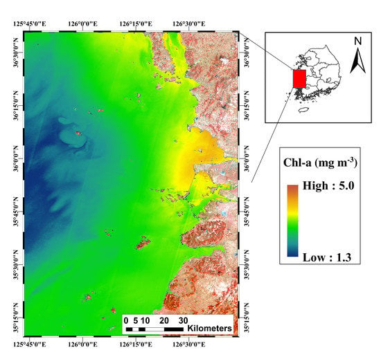
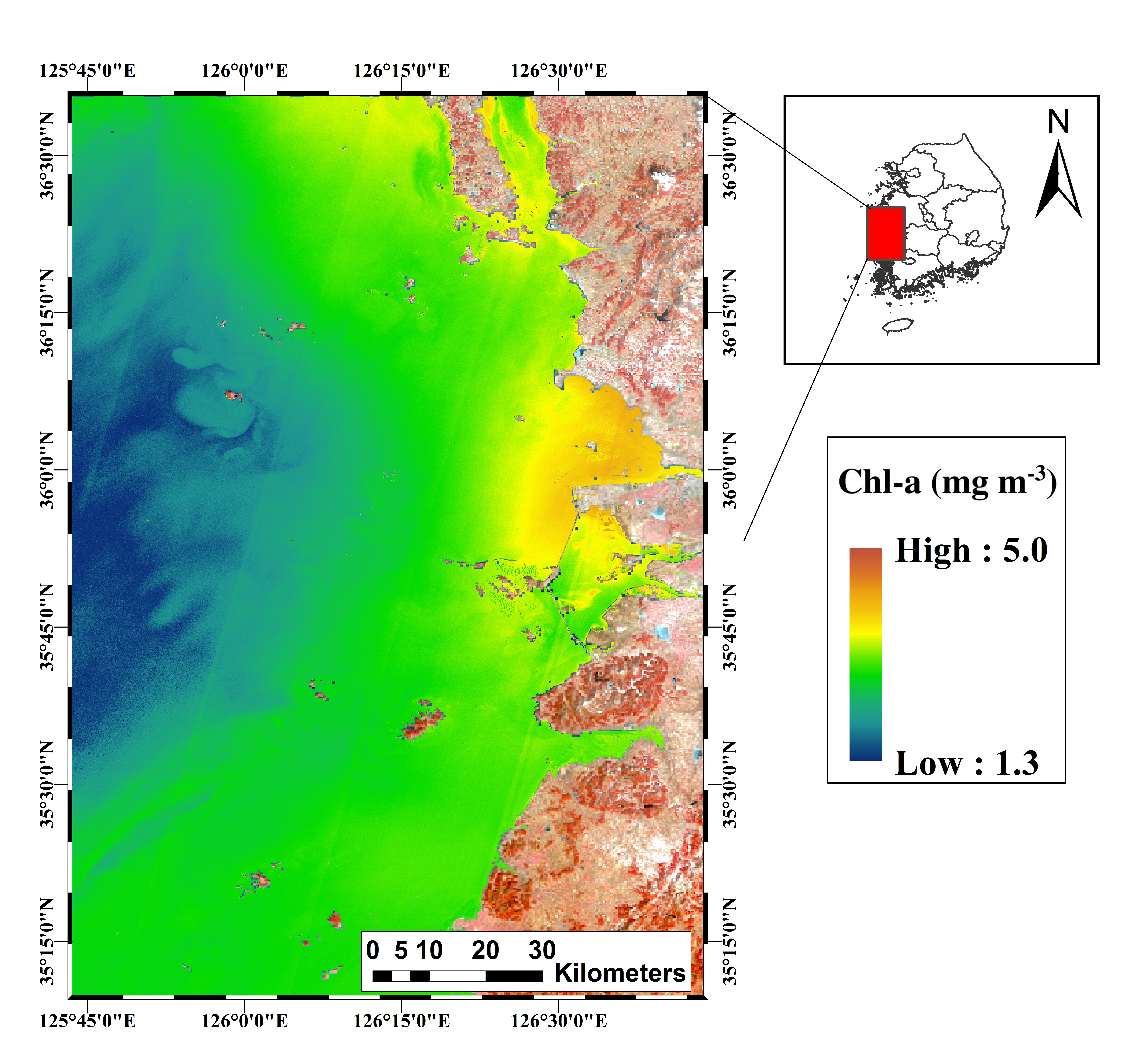
2. Study Area
The study area was part of the Korean West Sea, which is located in the eastern part of the Yellow Sea ( N, E; area of 10,705 km2) (Figure 1). The Yellow Sea is a shallow marine ecosystem with the average and maximum water depths of 44 m and 103 m, respectively [38]. There is clear seasonality in sea surface temperature (SST) over the Yellow Sea, where January is the coldest month with an average SST of 4–7 °C and July is the warmest, with an average SST of 26–27 °C [39]. There are a total of 339 fish species in the Korean West Sea [40]. Over the past few years, some fish species, such as small yellow croaker, hairtail, large yellow croaker, and flatfish have exhibited continuous declines due to overharvesting, degraded marine ecosystem quality, and several unknown factors [41].
The increase in the level of the eutrophication, as a result of human activities such as dense agricultural practices along the coastal area, is another reason for environmental pollution over the study area that have significant negative effects on marine ecosystems, such as fish death, and a loss of important protein for the people dependent upon them [1]. Furthermore, in the Yellow Sea waters, there are other constituents than phytoplankton, such as inorganic particles and dissolved organic matter that are the major obstacle for simple empirical algorithms to determine the statistical relationship between Chl-a concentration and spectral bands [42]. Additionally, a very limited number of studies have attempted to investigate the optical properties of the Yellow Sea, such as phytoplankton, from the ocean color images. As a result, monitoring the Chl-a concentration, as an important index to evaluate the extent of eutrophication, at fine resolution is a crucial task in this area.
3. Materials and Methods
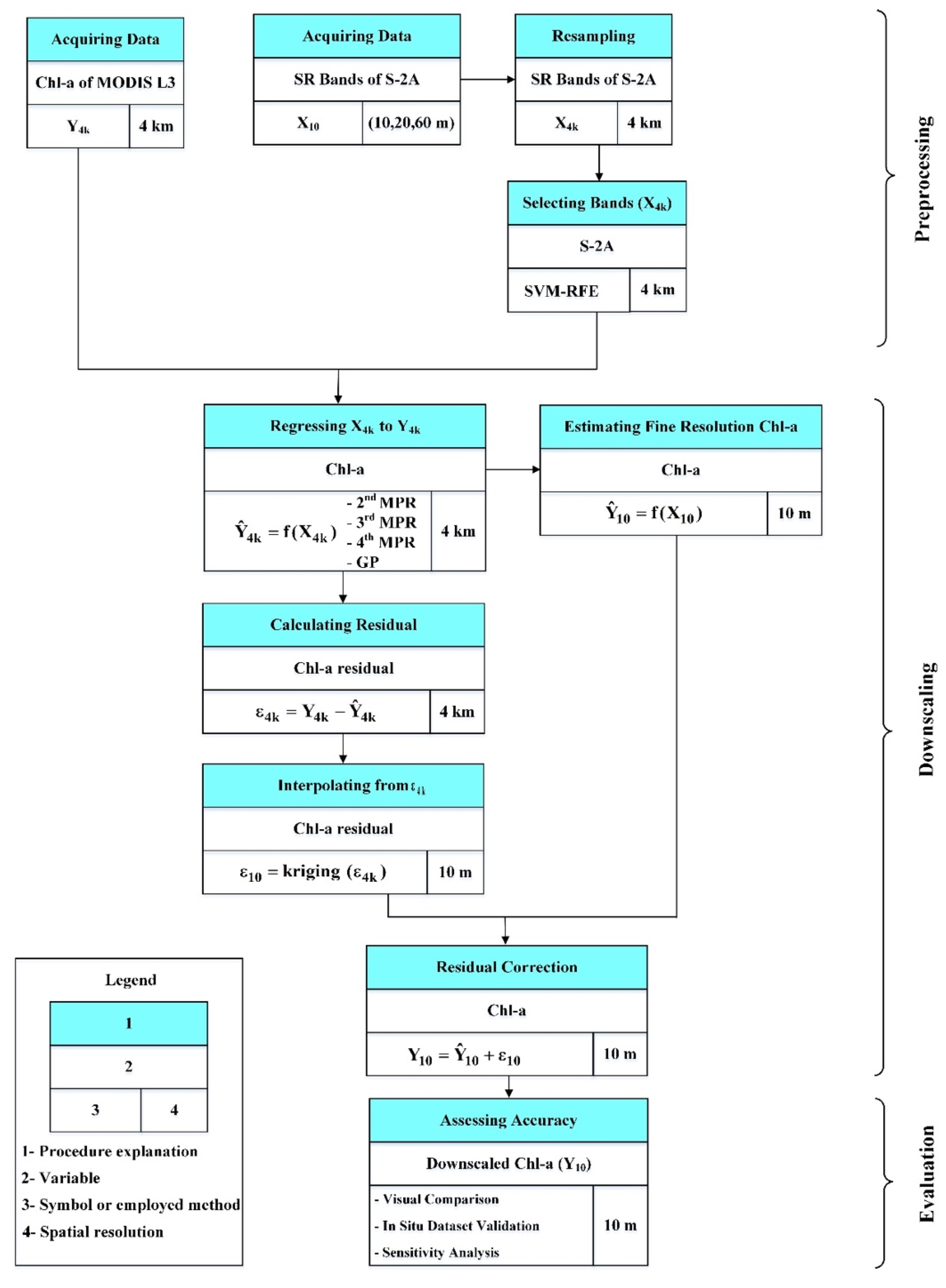
The main objective of this research was to develop an approach for MODIS Chl-a downscaling and produce Chl-a concentration maps for complex coastal regions. Figure 2 displays the detailed explanation of the procedure used. The downscaling approach was accomplished in four steps: (1) remote sensing data, including MODIS Chl-a at 4 km (defined as Y4k) and S-2A at 10 m (defined as X10), were acquired, and S-2A data were resampled to 4 km MODIS resolution (denoted as X4k); (2) the most important S-2A band combinations (X4k) were chosen by utilizing the support vector machine recursive feature elimination (SVM-RFE) method; (3) MODIS Chl-a downscaling from 4 km to 10 m was performed by regressing X4k to Y4k, calculating the residual at 4 km (), and adding the interpolated residual () to the estimated fine-resolution Chl-a (); (4) the obtained downscaled maps were compared with visual comparison, validated with in situ data, and all the applied methods were assessed using sensitivity analysis. A complete explanation of the aforementioned steps is described in Section 3.1, Section 3.2, Section 3.3, Section 3.4.
3.1. Data Description
In the current study, a downscaling approach was proposed based on GP and MPR techniques to produce high-resolution MODIS Chl-a data by relating coarse-resolution MODIS Chl-a data to high-resolution Sentinel-2A MSI (S-2A) data. There are some challenges associated with downscaling Chl-a: 1) MODIS Chl-a and S-2A measurements have different revisit times of 8 and 10 days, respectively; 2) in situ data used for validation of the downscaling model are irregularly distributed in space and rarely accessible; 3) to obtain reasonable results for downscaling Chl-a, a remote sensing image should have cloud coverage less than 10%. It has been reported that sea fog is frequently observed around the Korean peninsula with a maximum occurrence in the West Sea in summer with a mean frequency of 5.3 days in July [43]. The frequency is less than 1 day during fall and winter. Therefore, the above-mentioned challenges imposed some limitations for selection of images on every season. Hence, two MODIS and S-2A Level-1C (hereafter S-2A) datasets were acquired on February 2 (winter) and August 4 (summer) in 2016. All images had less than 10% cloud coverage and were almost concurrent with in situ measurements (±5 days).
The Chl-a concentration maps used in the current study were used from MODIS Chl-a concentration standard mapped images (SMIs) with a 4 km resolution. The SMIs were created from bands 13 (0.653 µm),14 (0.681 µm), and 15 (0.750 µm) of the MODIS sensor (hereafter referred to as MODIS Chl-a). Due to strong fluorescence signals from Chl-a at these spectral bands, these bands were suitable for the detection of the Chl-a concentration [44,45]. For retrieval of Chl-a concentration, the standard OC3/OC4 (OCx) band ratio algorithm combined with color index (CI) introduced by Reference [46] was implemented. The MODIS Chl-a data were obtained from the Giovanni website (https://giovanni.gsfc.nasa.gov/giovanni/).
S-2A band images (Table 1) for high-resolution data were acquired from the Copernicus Open Access Hub (https://scihub.copernicus.eu/). S-2A products include 13 bands with the top-of-atmosphere (TOA) Reflectance. All bands were processed by radiometric and geometric correction using a UTM/WGS84 projection. Recent studies have reported that S-2A is more powerful than Landsat 8 OLI in distinguishing areas affected by algal blooms because S-2A has three near-infrared (NIR) bands and Landsat 8 OLI has only one NIR band [47,48,49,50,51]. The three additional NIR bands of S-2A make it feasible to develop more suitable algorithms for the retrieval of the Chl-a concentration in intense bloom conditions [52].
The in situ Chl-a measurements used in the analysis were obtained for seven stations from the Korea Institute of Ocean Science and Technology (KIOST) website (http://joiss.kr). The locations of the stations are shown in Figure 1. Multidepth sampling was used to collect water samples from the surface layer (0–15 cm depth). A fairly large water sample was collected and the sample was filtered to concentrate the chlorophyll-containing organisms followed by mechanical rupturing of the collected cells, and extraction of the chlorophyll from the disrupted cells into the organic solvent acetone. The extract was then analyzed by a spectrophotometric method using fluorescence. Therefore, to validate the downscaling models, a total of 14 samples at two depths (Table 2) were employed. The remote sensing and in situ data acquisition dates are shown in Table 2, with in situ data from 1 February 2016, corresponding to remote sensing data from 2 February 2016, and in situ data from 1 August 2016, corresponding to remote sensing data from 4 August 2016.
3.2. Preprocessing
The image preprocessing methods the same as (1) MODIS gap filling, (2) resampling, (3) land-water separation, and (4) subsetting were used to prepare all satellite images for further processes. Then, feature selection was employed to determine the most important band combinations for Chl-a prediction. First, the grid-fill method [53] was used to fill the missing values in the MODIS Chl-a images. This software has high computational efficiency and fills missing values in an iterative relaxation scheme using Poisson’s equation. For validation, random removal of the original Chl-a pixel values was conducted to provide data to validate the grid-fill method. For this purpose, 5% of the original data were deleted from the outside boundary of the study region and preserved for cross-validation. Then, the corresponding values of the deleted data were estimated by utilizing the grid-fill method, and the difference between the original pixel values and the reconstructed values was evaluated. Consequently, the spatial distribution of Chl-a concentrations was produced.
At the second step, all S-2A images were mosaicked and then resampled to a resolution of 10 m (X10). Since the study region had a remarkable number of islands (Figure 1), the reflectance caused by islands could decrease the accuracy of the applied models. Therefore, the third step of preprocessing aimed to separate water from land pixels to improve the downscaling results. The most commonly used indices, namely, the normalized difference vegetation index (NDVI) and normalized difference water index (NDWI), have already been employed for land-water separation purposes [54,55,56,57,58]. In the current study, land-water separation was performed by utilizing the NDWI index. The formula of this index is as follows:
where and are the green and near-infrared (NIR) reflectances of S-2A with 10 m resolution. Based on the NDWI computed images, water pixels have positive values, while negative pixels are usually classified as vegetation or soil features.
At the fourth step, the study area boundaries were used to produce a spatial subset of both MODIS Chl-a and S-2A images, and the S-2A dataset was resampled from 10 m (X10) to 4 km resolution of MODIS Chl-a (X4k) using the nearest neighbor method [59]. Then, MODIS Chl-a and S-2A images at 4 km (Y4k and X4k) were used as dependent and independent variables, respectively, to develop GP and MPR models. Additionally, the developed models were applied to S-2A images at 10 m (X10) to estimate downscaled Chl-a at 10 m spatial resolution.
At the fifth step, the SVM-RFE feature selection method was employed to specify the most important bands of the S-2A dataset (X4k). This method is a widely used technique for feature selection that has been utilized in a wide variety of remote sensing research studies [60,61,62]. To perform feature selection, multiple mathematical operations, including multiplication, addition, subtraction, rationing, averaging, and square transformation, were used to calculate 597 various combinations of the resampled S-2A bands at 4 km, and the computed combinations served as the input for the feature selection method. Then, SVM-RFE was trained on the calculated dataset using the MODIS Chl-a concentration (Y4k) and S-2A band combinations (X4k) as the predictand and predictor variables, respectively. As a result, relevant combinations for the downscaling procedure were chosen.
3.3. Downscaling
The downscaling model used in the current study was a regression-based approach considering the statistical relationship between MODIS Chl-a and S-2A bands at 4 km and 10 m spatial resolution. The straightforward formulation of this relationship is expressed as in Equation (2).
where X is the selected S-2A bands (predictor variables) at 4 km (X4k) and 10 m (X10), is the estimated MODIS Chl-a at 4 km () and 10 m (), and f represents a nonlinear regression function developed by GP and MPR techniques.
First, a relationship between Y4k and X4k was established using all the applied methods as 2nd-degree MPR, 3rd-degree MPR, 4th-degree MPR, and GP. From the 636 pixels of the independent (X4k) and dependent (Y4k) variables, 445 pixels were used for training, and the remaining 191 pixels were reserved for the validation of the models. Standardization was a prerequisite step before training all the applied methods to ensure that all variables remained on the same scale. Therefore, the standardization of all independent variables (X4k) in the training and validation set was performed by subtracting the mean and dividing by the standard deviation of the training set. This preprocessing sped up the convergence and allowed efficient training of the network. Then, the estimated Chl-a at 4 km () was subtracted from the original MODIS Chl-a at 4 km (Y4k) as follows:
where is the low-resolution residual at 4 km.
A simple kriging interpolation technique [63,64] was utilized to interpolate the to 10 m resolution () using the center points of the MODIS Chl-a pixels. Finally, to produce the downscaled map of Chl-a at 10 m resolution (), the developed model as in Equation (2) was added to , which is expressed in the function below (Equation (4)):
3.4. Sensitivity Analysis
For a given mathematical model, a sensitivity analysis (SA) measures how much the uncertainty and fluctuations of the input variable contribute to the outputs or performance of the system. In general, SA may be performed by two different techniques, local and global SA, with the former exploring the important model factors for a given set of factor values, and the latter apportioning the uncertainty in outputs to the uncertainty in each input factor to identify the important factors [65]. In the current study, the Morris method [66], as the most widely used global SA method, was employed to quantify the sensitivity of the GP and MPR models. This method is also called the once-at-a-time (OAT) method because, in each run, a new value is assigned to only one input variable. To carry out SA, the Morris sensitivity measure index () was used as in Equation (5):
where i is the number of input variables, r is the number of sample points in the parameter space (indexed n) and EEi,n is the elementary effects (EEs) assessed for the i-th input variable using the n-th sample point. EEs are employed to specify noninfluential inputs for a computationally costly mathematical model or for a model with a great number of input parameters, where the costs of evaluating other SA methods such as variance-based methods are not reasonably priced.
3.5. Mathematical Background
3.5.1. Multiple Polynomial Regression
The polynomial model is a form of a regression method that can be used when the relationship between an independent and dependent variable is curvilinear [67]. The nth order polynomial model with one variable Equation (6) is the general form of the polynomial model that indicates the nonlinear relationship between one predictand and one predictor variable.
where , , …, are the unknown regression coefficients and is random error. Furthermore, MPR can also be defined with different degrees. For instance, a quadratic (second-order, n = 2) polynomial model can be given as in Equation (7).
To select the best model between different MPR degrees for MODIS Chl-a downscaling, three degrees of models, including second-order (2nd), third-order (3rd), and fourth-order (4th), were trained and compared.
3.5.2. Genetic Programming
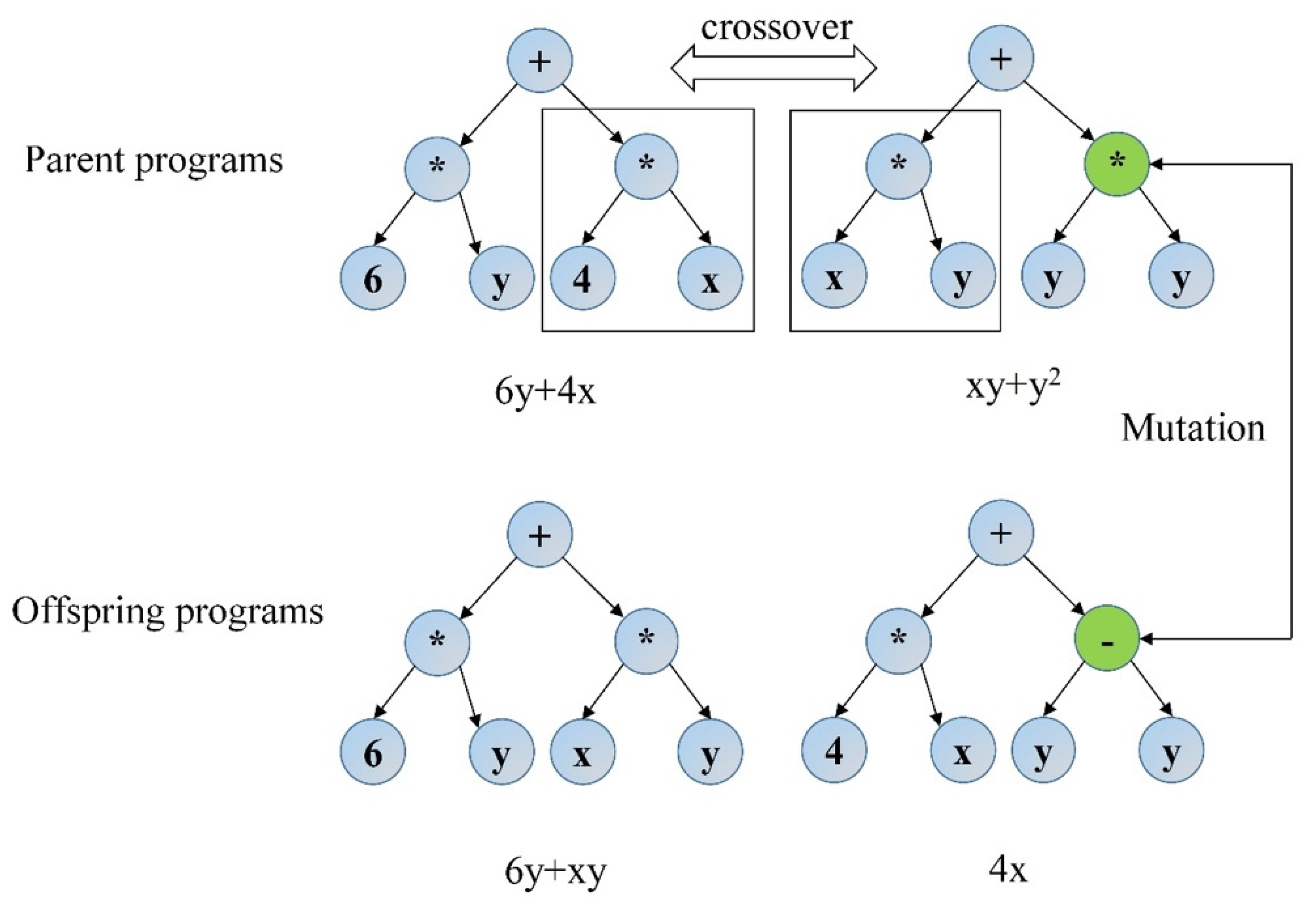
GP is one of the most recent data-driven techniques developed by Koza [68] and is a collection of techniques for finding a highly fit individual in the space of possible solutions. In GP, individuals are mathematical formulas created by combinations of functions (e.g., sin, cos, ÷, ×, +) and variables (e.g., x, y, 6). Each individual takes the role of a possible solution for a given problem. Figure 3 shows four simple formulas (individuals) created by functions and variables as an example. Each individual has its fitness value to optimize. GP applies evolutionary computation to find the best individual for optimized fitness values.
Generally, the GP technique follows four steps to find the fittest individual: (1) an initial random population of individuals composed of functions and variables is created; (2) the fitness of each individual in the population is validated with a problem-specific fitness function, and the most appropriate individuals are selected to survive in the new population as parents; (3) once parents are selected, they create better types known as offspring or new generations by producing algorithms known as genetic operators (i.e., crossover, mutation, and duplication); (4) then, the individuals are assessed for fitness; (5) the process from (2) to (4) is repeated over many generations until an individual satisfies a given success criterion (e.g., the number of generations exceeds the specified number of iterations).
Figure 3 illustrates the crossover and mutation operations in GP. Individuals in GP are shown in tree form with different characteristics, such as size, shape, and content. The crossover and mutation operations are performed to produce new offspring (the panels in the lower row) from the parent (the panels in the upper row). Additionally, Figure 3 displays how crossover and mutation change the final functions and eliminate an input variable y at the second offspring (the lower right panel).
In the current study, the gplearn package [69] in Python software was used for GP implementation. In general, GP has two major parameters (population size and generation size) that should be optimized to generate high performance. The optimum values of the mentioned parameters were computed by utilizing the harmony search (HS) algorithm introduced by Geem, et al. [70] using 10-fold cross-validation. For more information about the HS method, readers are referred to Geem, Kim and Loganathan [70] and Lee and Singh [59].
4. Results
4.1. Preprocessing
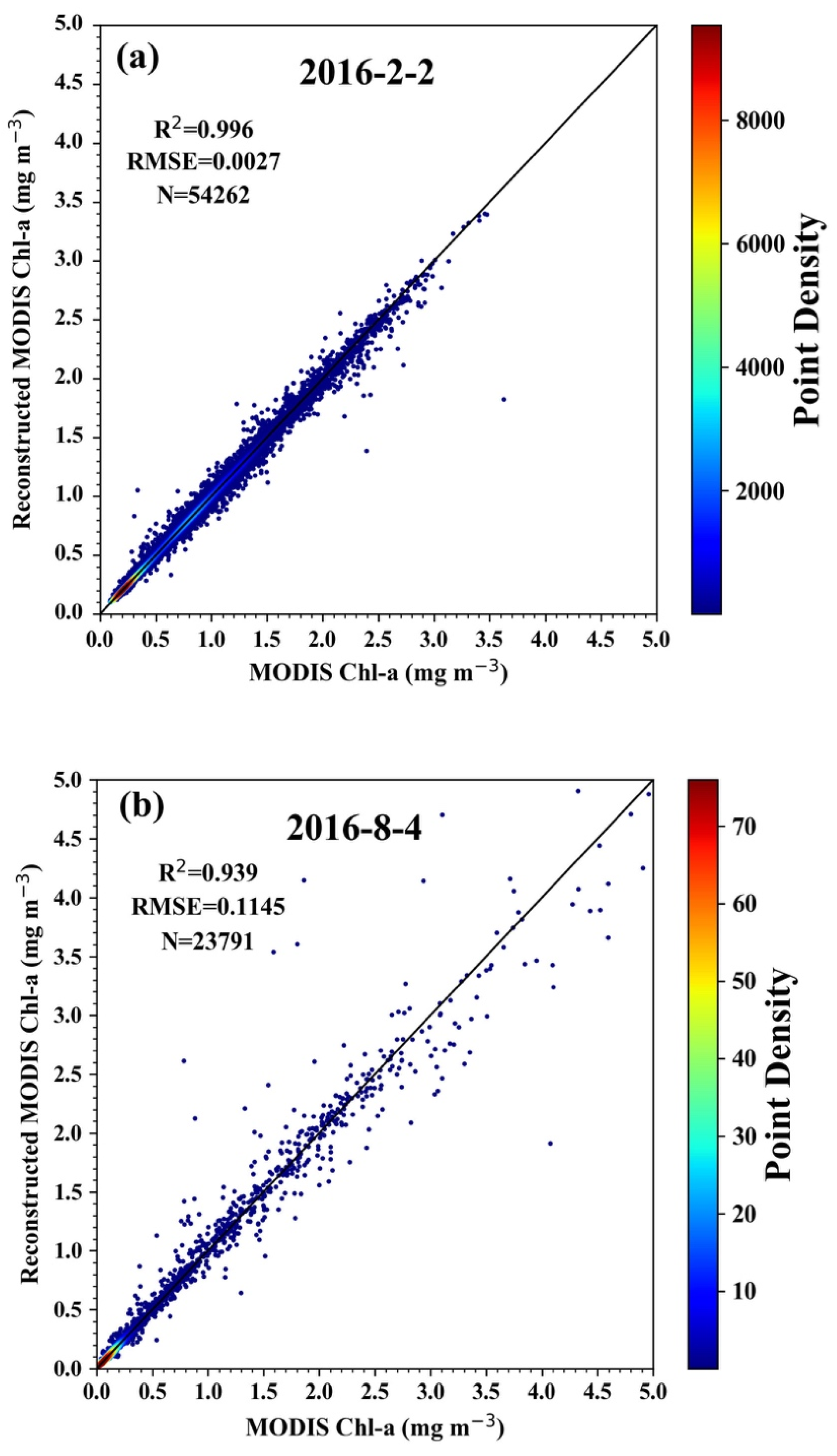
The scatter plots between the original MODIS Chl-a and their reconstructed values with the grid-fill method are shown in Figure 4. According to the results, a good match between the original MODIS Chl-a and their filled values can be seen with R2 = 0.996 for winter (panel (a)) and R2 = 0.939 for summer (panel (b)). Therefore, it can be concluded that the grid-fill method exhibits good performance for the reconstruction of MODIS Chl-a values. Note that the reason for the better performance of the method on the winter day than on the summer day might be related to the presence of more missing values in the selected scene of the summer day that occurs due to high cloudiness on the summer day.
The most important combinations of S-2A images, among the 597 cases, were chosen by utilizing the SVR-RFE method. Four high-ranked combinations were selected as the final variables, namely, B1/B3, B2/B3, B1/(B3+B4), and B2/(B3+B4). These selected predictors are a combination of bands 1 (Coastal aerosol), 2 (Blue), 3 (Green), and 4 (Red).
4.2. Downscaling Results
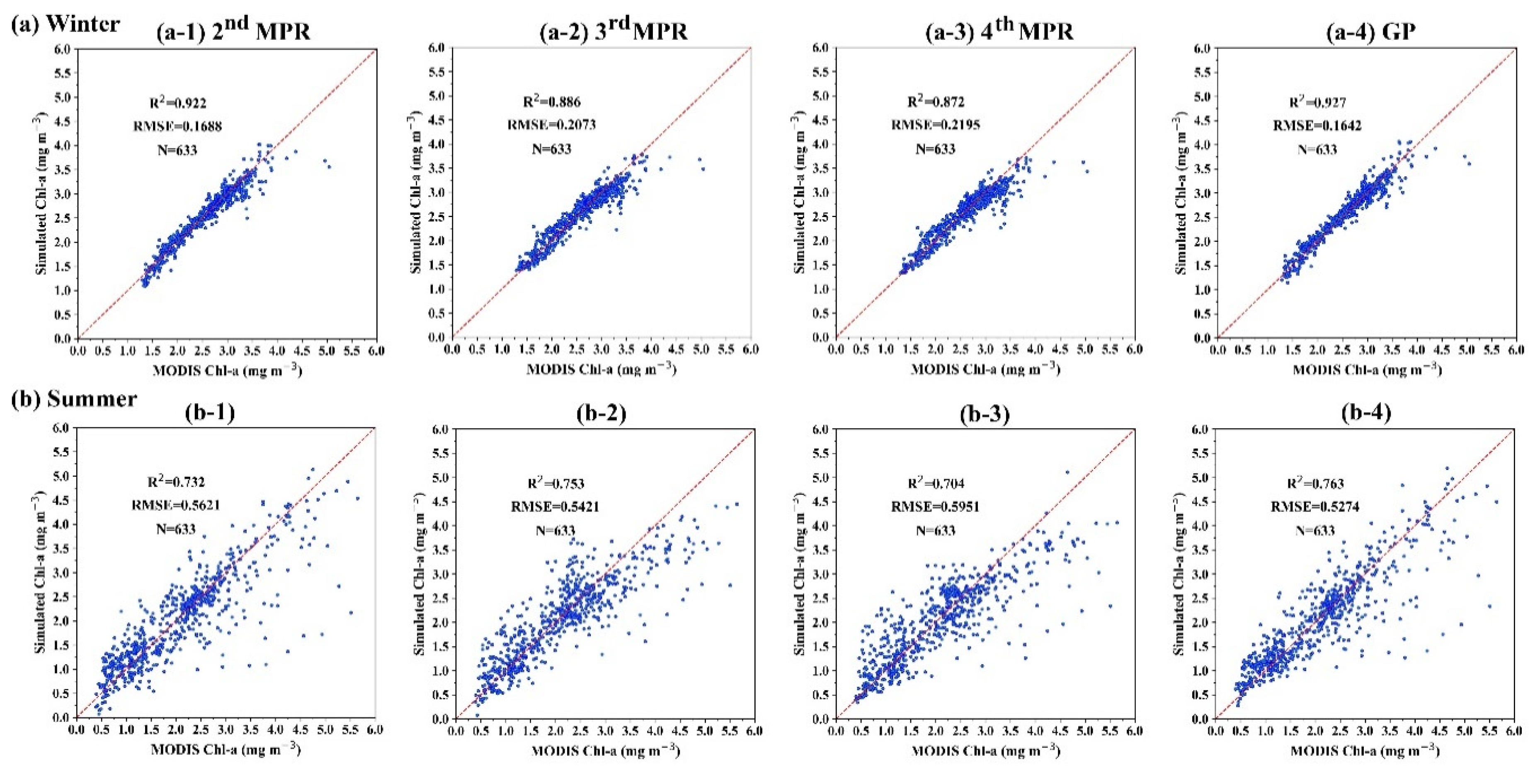
For downscaling, MPR with three degrees (2nd, 3rd, and 4th) and GP were trained with the four determined band combinations as predictors and MODIS Chl-a as a predictand at low-resolution (4 km). Then, a residual correction was performed utilizing the described methodology in the downscaling section (Section 3.3), and Equations (3)–(4) to produce high-resolution Chl-a maps (Y10). To assess the accuracy of the downscaling technique, the final downscaled maps (i.e., Y10) were validated with the original MODIS Chl-a maps at a pixel size of 4 km. For this purpose, sample values were extracted from the downscaled maps (Y10) within a 3 × 3 window around the center of each MODIS Chl-a pixel, and the mean of each sample was calculated and compared with the original MODIS Chl-a (Figure 5 and Table 3).
On the winter day, as shown in Table 3, the performance measurements of the GP model were slightly better than those of the 2nd-degree MPR. According to the performance indices, the accuracy of the models was ranked as GP > 2nd-degree MPR > 3rd-degree MPR > 4th-degree MPR for the winter day. For the summer day, the rank was GP > 3rd-degree MPR > 2nd-degree MPR > 4th-degree MPR. Overall, the GP exhibited the best performance for the winter and summer days.
This finding shows the superiority of GP over the MPR method with different degrees of Chl-a downscaling. The possible reason for this result might be related to the flexible structure of the GP model compared with the fixed formulation of MPR models. While MPR models use a fixed form to define the relationship between the predictor and predictand variables, the evolution process in GP allows its function to take any feasible formulation. This flexibility gives GP the ability to adopt any form of functions to capture various relationships between the predictor and predictand variables, even highly nonlinear relations. Therefore, this unique feature of GP increases the probability of finding the best relationship in the downscaling procedure, resulting in a better prediction than the MPR models.
The accuracy of the models is presented in Figure 5. The best match between the MODIS Chl-a and simulated values can be seen in the GP model (see the panels in the fourth column in Figure 5), with R2 = 0.927 and RMSE = 0.1642 on the winter day, compared to the MPR models (2nd-, 3rd-, and 4th-degree). The same result can be seen on the summer day (the best performance in the GP model), as shown in the bottom panels of Figure 5. Furthermore, it can be seen that all the applied models estimate Chl-a better at lower concentrations than at higher concentrations, particularly in the range of 1.5–3.5 mg m−3, as presented in Figure 5.
4.3. Model Evaluation
4.3.1. Visual Comparison
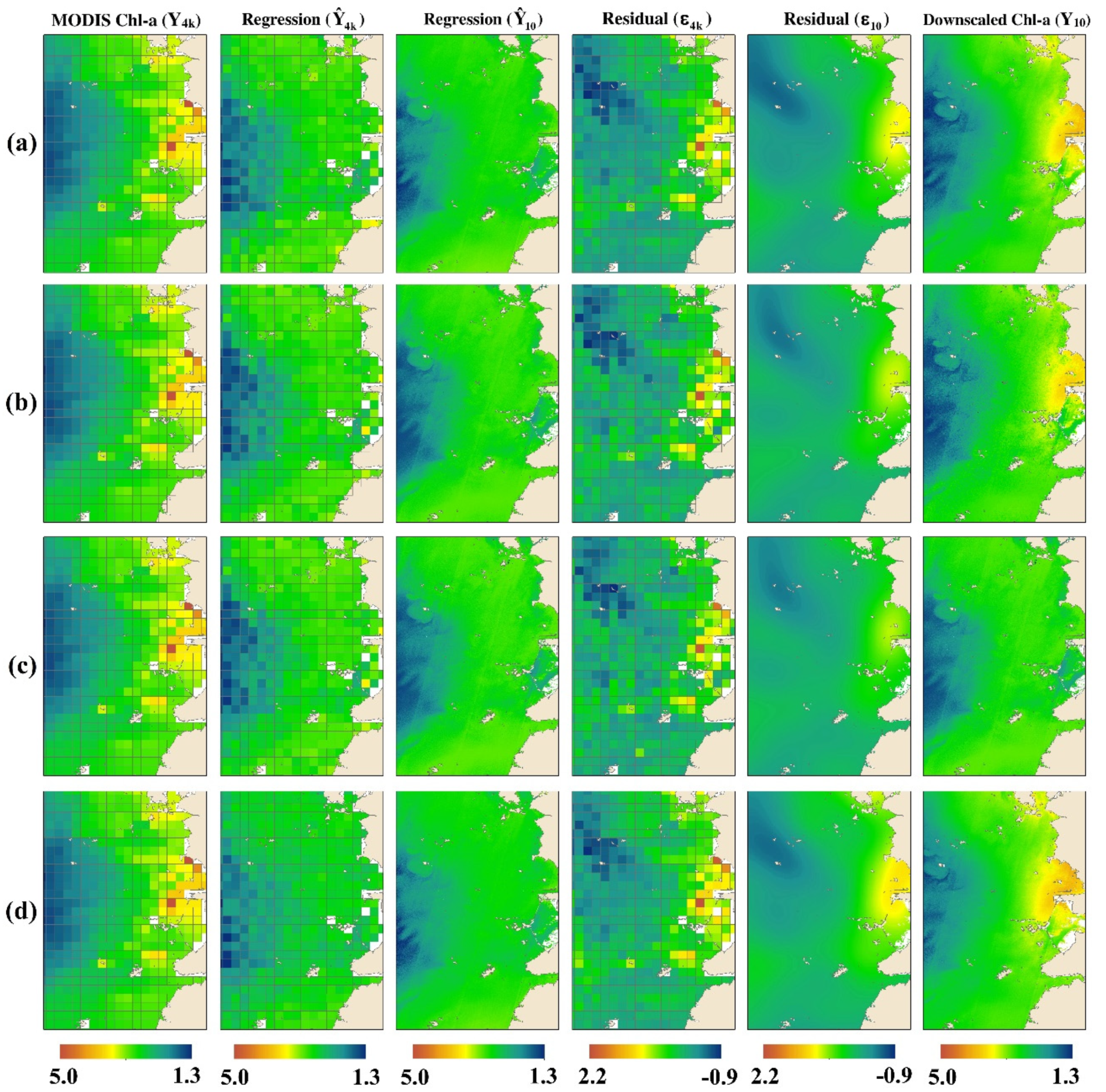
The detailed maps of the downscaling approach for the winter and summer days are shown in Figure 6 and Figure 7, respectively. The good agreement between the original MODIS Chl-a (the panels in the first column in Figure 6) and the estimated Chl-a maps (the panels in the last column in Figure 6) can be seen for the GP and 2nd-degree MPR. From Figure 6, the major trend of Chl-a is fairly modeled with GP and 2nd-degree MPR but specific and substantially high values are not captured in both models such as the values in the near coastal area. However, the residual model can additionally capture this high variability and produce a reliable estimate in the final stage, as seen in the last column of Figure 6. According to the results illustrated in Table 3, and the panels in the last column of Figure 6, 4th-degree MPR cannot estimate the Chl-a values at 10 m resolution as accurately as the other models, especially in coastal areas. This phenomenon indicates that the GP and 2nd-degree MPR can capture the most variation in high Chl-a concentrations at 4 km resolution.
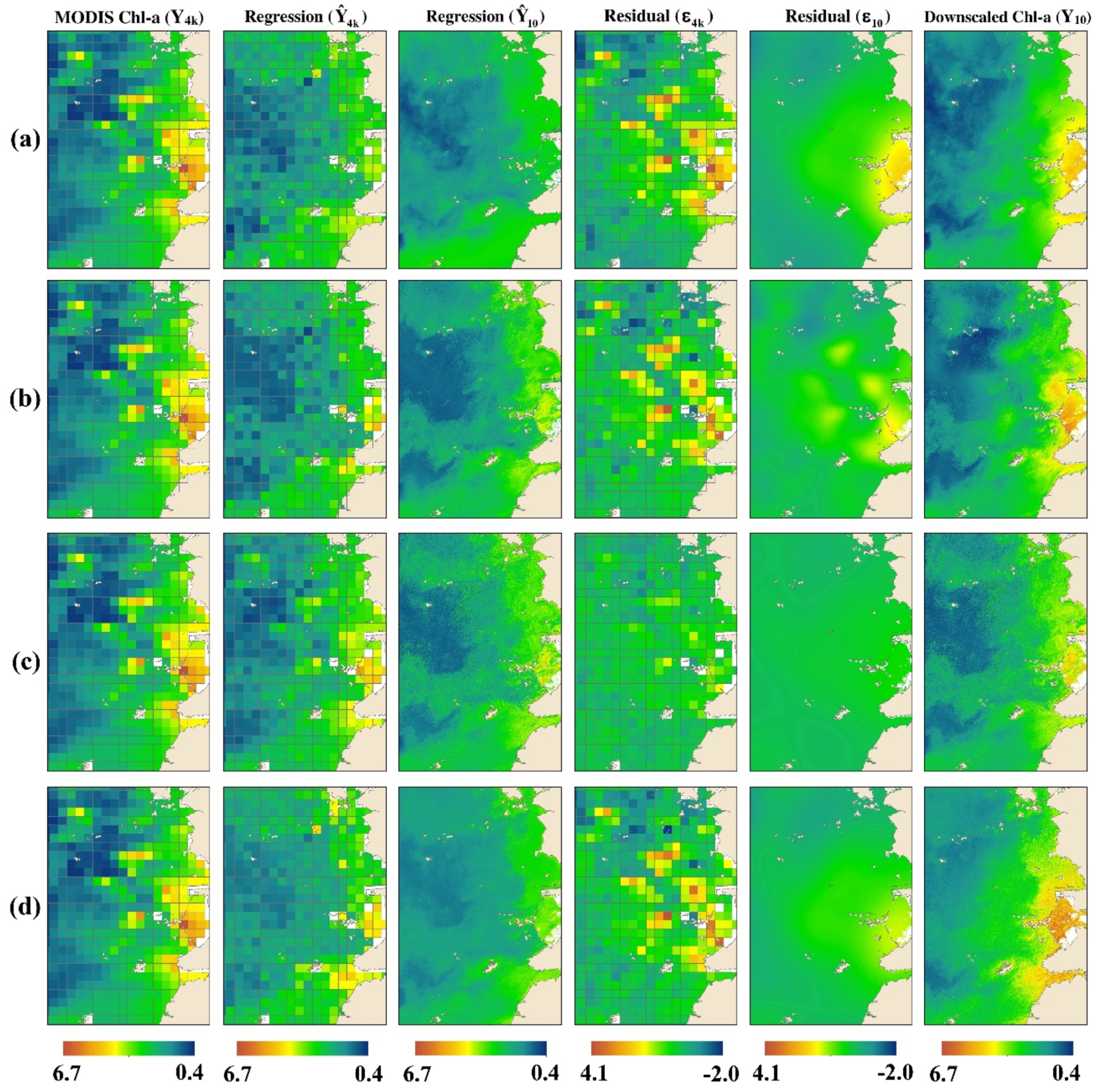
By estimating the Chl-a concentrations on the summer day, similar model behaviors became obvious on the summer day compared to the winter day (Figure 7). Among all the applied models, GP estimations in coastal areas showed better agreement with the original MODIS Chl-a on both the winter and summer days than all the applied MPR models. Since coastal areas play a vital role in marine ecosystems and human health, GP estimations are considerable for water quality monitoring in coastal areas.
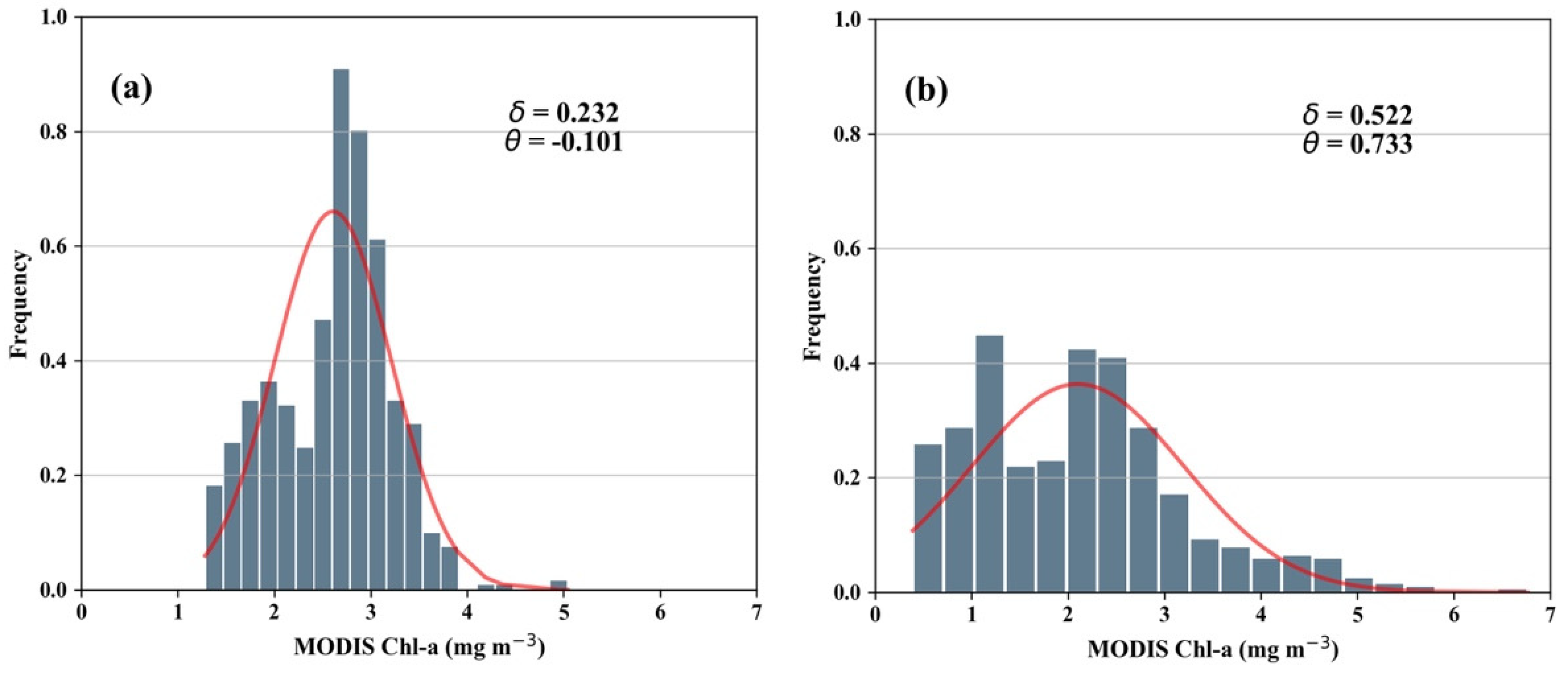
From Figure 7, the simulation results became worse in the sea (the second and last column panels in Figure 7), and all models tended to underestimate some high Chl-a values. The possible reason for this result might be the higher spatial variability of the MODIS Chl-a concentration on the summer day than on the winter day (Figure 8), which is different from the normal distribution (, ). Therefore, all the applied models did not fairly estimate the Chl-a values in the sea, and their accuracy decreased on the summer day compared to that on the winter day (Figure 5 and Table 3). From Figure 6 and Figure 7, the Chl-a concentration gradient follows a similar pattern with water depth in all maps, and its concentration decreases as water depth increases. Therefore, the region close to the seashore shows a high Chl-a concentration, while the region in the sea presents a low concentration of Chl-a.
4.3.2. In Situ Validation
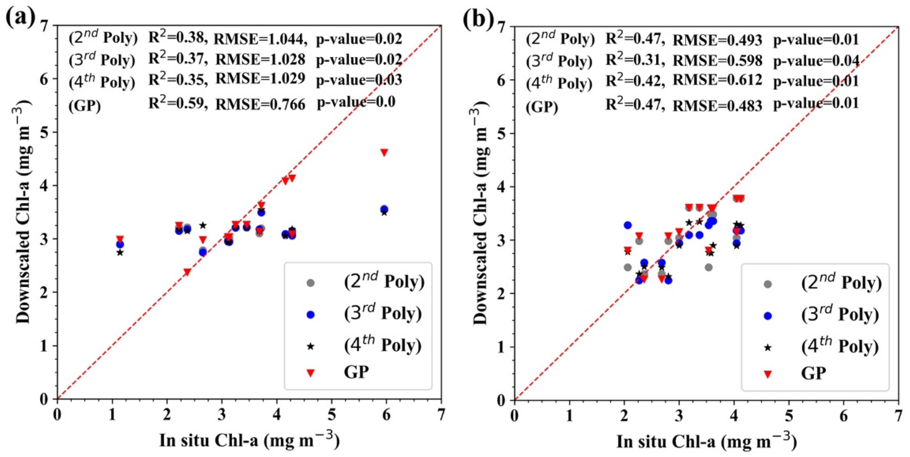
The results of the downscaling models were assessed with the in situ Chl-a data of seven stations along the study area (Figure 1) to validate model performances. For this purpose, sample values were extracted within a 3 × 3 window around the center of each station point, and the mean of each sample was calculated and compared with the in situ data. The results in terms of the R2 and RMSE are presented in Figure 9 for the winter day (left panel) and the summer day (right panel). The computed p-values (Figure 9) shows that R2 of all models is statistically significant (p-values lower than 0.05). In general, the R2 of the GP model was higher than that of the other models for the winter and summer days, which were 0.59 and 0.47, respectively, as shown in Figure 9. Additionally, the RMSE of the GP model was smaller than that of the other models for the winter and summer days, at 0.766 and 0.483, respectively.
These results indicate that the GP model can estimate Chl-a concentrations more accurately than the other models on both winter and summer days. From Figure 5 and Figure 9, one can see that the validation of the downscaling models with the original MODIS Chl-a and the in situ data provides different levels of accuracy. This discrepancy shows the uncertainties in remote sensing data, indicating that the performance of the downscaling model is greatly affected by the accuracy of the remote sensing reflectance.
4.3.3. Sensitivity Analysis
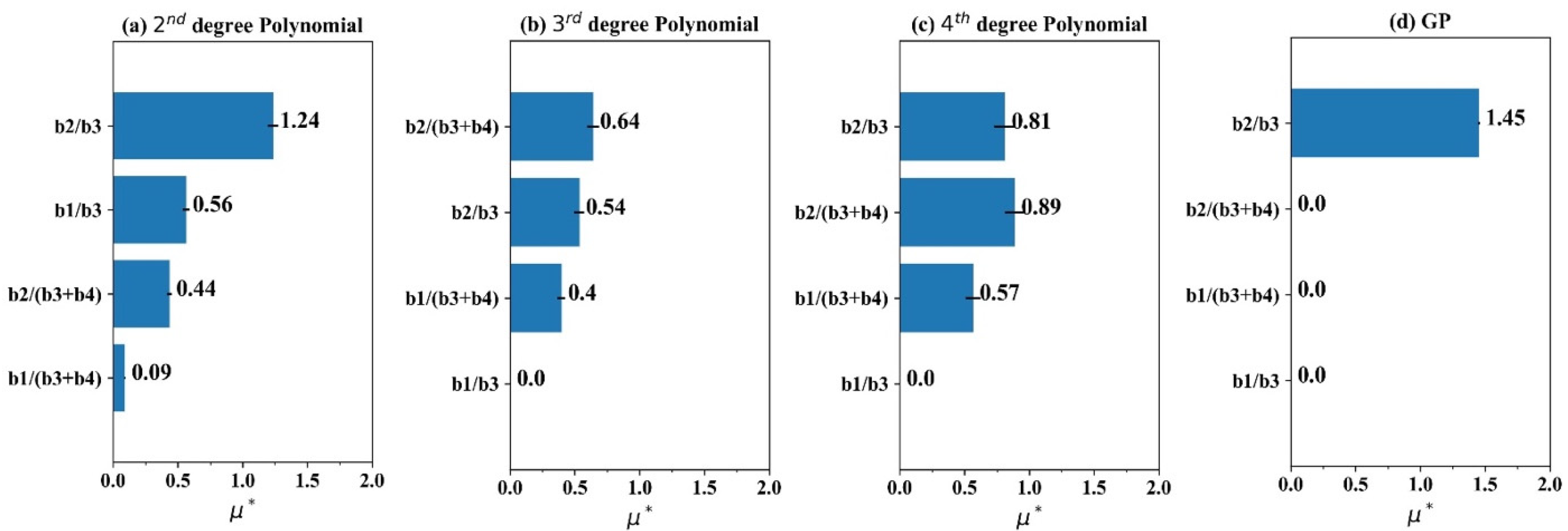
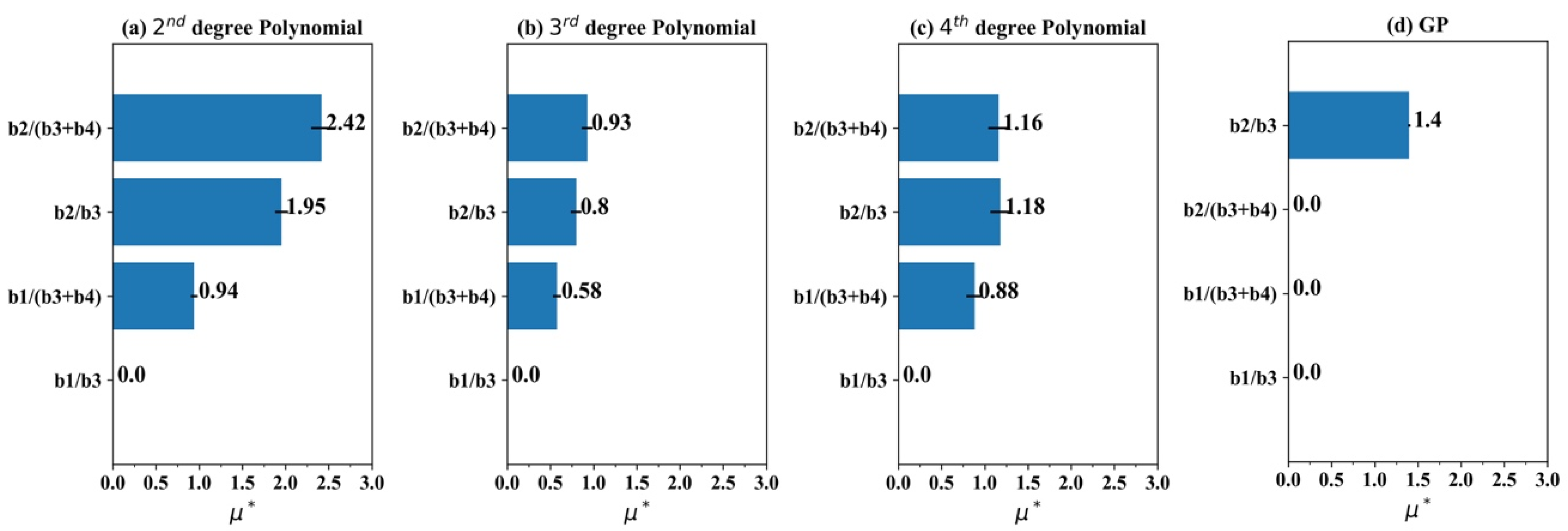
To explore the sensitivity of the applied models to the changes in input parameters, the sensitivity measure index () was calculated, as shown in Equation (5), for all predictor variables on both winter and summer days (Figure 10 and Figure 11). The results of SA indicate that all the applied models are sensitive to the surface reflectance changes ( values range from 0 to 1.45 for the winter and 0 to 2.42 for the summer day), and this sensitivity varies between the applied models. Figure 10 and Figure 11 show that the 2nd-degree MPR model is the most sensitive model ( values ranged from 0.09 to 1.24 for the winter and 0.94 to 2.42 for the summer day), while the GP model is the least sensitive model ( = 1.45 and 1.4 for B2/B3 band combination in winter and summer days, respectively) to the changes in the predictor variables. In addition, the sensitivity of the MPR models increases on the summer day compared to that of the winter day, while the GP model shows a slight decrease to the changes of the B2/B3 band combination on the summer day compared to that of the winter day.
It can be concluded that although GP and 2nd-degree MPR show comparable accuracy (Figure 5 and Table 3) on both winter and summer days, the GP model with the least sensitivity to the changes in the input parameters is more effective than the 2nd-degree MPR for downscaling Chl-a. Additionally, SA results show that the accuracy of all models is strongly related to the accuracy of the remote sensing data; this further confirms the need for atmospheric correction as an essential task in the downscaling procedure [71].
5. Discussion and Conclusions
In the current study, a downscaling framework composed of GP and MPR models was developed to downscale MODIS Chl-a from 4 km to 10 m pixel size using S-2A band combinations at 10 m as predictor variables. The MODIS Chl-a at 4 km was downscaled in four main steps: (i) acquiring MODIS Chl-a and S-2A images at 4 km and 10 m, respectively; (ii) applying feature selection to select the most important S-2A band combinations as predictor variables; (iii) employing the trained MPR with three degrees (2nd, 3rd, and 4th) and GP model to downscale MODIS Chl-a; (iv) assessment of the results with original MODIS Chl-a maps at a pixel size of 4 km and in situ measurements.
By comparing the performance of all the models applied for downscaling, the GP model presents more accurate results and less sensitivity to the changes in all variables for downscaling Chl-a. The superiority of the GP model over MPR models is related to the flexible formulation structure of the GP compared to the fixed formulation of the MPR models. The flexible structure of the GP allows its function to take any feasible formulation so that it increases the probability of finding the best input-output relationship between thousands of formula. Visual comparison of the applied models showed that although the major trend of Chl-a is fairly modeled with GP and 2nd-degree MPR, but specific and substantially high values are not captured with both models such as the values in near coastal areas. This drawback of the models can be solved with the residual correction that makes it an essential procedure to improve the accuracy of the spatial downscaling model.
Among all the applied models, the GP model provided better estimations in coastal areas than all the MPR models. Therefore, GP can serve as a feasible alternative model to estimate Chl-a concentrations in coastal areas with complex characteristics, where water quality monitoring plays a vital role in the protection of marine ecosystems and human health. Moreover, the results indicate that the performance of the models greatly depends on the spatial variability of the MODIS Chl-a concentration. Its distributional characteristics (e.g., normal or skewed) can be a good option for model selection criteria. Therefore, to ensure the validity of the GP model in other coastal areas, it is recommended to assess the normality to select the GP model for spatial downscaling of the MODIS Chl-a.
Although the downscaling procedure used in the current study was applied on two selected days, one in winter and one in summer based on data availability, it produced reasonable results due to using the S-2A dataset with 10 m spatial resolution. Future studies can be focused on extending this procedure at a higher temporal resolution. In addition, more research can be conducted with deep learning techniques for downscaling Chl-a concertation. In addition to the surface reflectance, more predictors such as NDVI and NDWI, due to the strong Chl-a absorption at red-NIR spectral regions, may be used in determining Chl-a concentration.
Author Contributions
H.M. initiated the idea and contributed to the analysis of the data and writing of the manuscript. T.L. secured funding for the project and contributed to the writing of the manuscript. J.Y. made revisions to the manuscript. All authors have read and agreed to the published version of the manuscript.
Funding
This research was funded by National Research Foundation of Korea (NRF), grant number 2018R1A2B6001799.
Acknowledgments
The authors would like to thank NASA and the ESA (European Space Agency) for providing the MODIS and Sentinel-2A MSI data, respectively. Additionally, we appreciate the Korea Institute of Ocean Science & Technology (KIOST) for providing Chl-a measurements of the western coast of South Korea. We would like to thank the three anonymous reviewers, whose comments significantly improved the paper.
Conflicts of Interest
The authors declare no conflict of interest.
References
- Bierman, P.; Lewis, M.; Ostendorf, B.; Tanner, J. A review of methods for analysing spatial and temporal patterns in coastal water quality. Ecol. Indic. 2011, 11, 103–114. [Google Scholar] [CrossRef]
- Blondeau-Patissier, D.; Gower, J.F.; Dekker, A.; Phinn, S.; Brando, V. A review of ocean color remote sensing methods and statistical techniques for the detection, mapping and analysis of phytoplankton blooms in coastal and open oceans. Prog. Oceanogr. 2014, 123, 123–144. [Google Scholar] [CrossRef] [Green Version]
- Cullen, J.J. The deep chlorophyll maximum: Comparing vertical profiles of chlorophyll a. Can. J. Fish. Aquat. Sci. 1982, 39, 791–803. [Google Scholar] [CrossRef]
- Guan, X.; Li, J.; Booty, W.G. Monitoring lake simcoe water clarity using Landsat-5 TM images. Water Resour. Manag. 2011, 25, 2015–2033. [Google Scholar] [CrossRef]
- Carpenter, S.R.; Caraco, N.F.; Correll, D.L.; Howarth, R.W.; Sharpley, A.N.; Smith, V.H. Nonpoint pollution of surface waters with phosphorus and nitrogen. Ecol. Appl. 1998, 8, 559–568. [Google Scholar] [CrossRef]
- Smith, V.H. Cultural eutrophication of inland, estuarine, and coastal waters. In Successes, Limitations, and Frontiers in Ecosystem Science; Springer: New York, NY, USA, 1998; pp. 7–49. [Google Scholar]
- Kar, D. Epizootic Ulcerative Fish Disease Syndrome; Academic Press: Cambridge, MA, USA, 2015. [Google Scholar]
- Bacher, C.; Grant, J.; Hawkins, A.J.; Fang, J.; Zhu, M.; Besnard, M. Modelling the effect of food depletion on scallop growth in Sungo Bay (China). Aquat. Living Resour. 2003, 16, 10–24. [Google Scholar] [CrossRef]
- Huot, Y.; Babín, M.; Bruyant, F.; Grob, C.; Twardowski, M.S.; Claustre, H. Does chlorophyll a provide the best index of phytoplankton biomass for primary productivity studies? Biogeosci. Discuss. 2007, 4, 707–745. [Google Scholar] [CrossRef] [Green Version]
- Goetz, S.J.; Gardiner, E.P.; Viers, J.H. Monitoring freshwater, estuarine and near-shore benthic ecosystems with multi-sensor remote sensing: An introduction to the special issue. Remote Sens. Environ. 2008, 112, 3993–3995. [Google Scholar] [CrossRef]
- Kutser, T. Passive optical remote sensing of cyanobacteria and other intense phytoplankton blooms in coastal and inland waters. Int. J. Remote Sens. 2009, 30, 4401–4425. [Google Scholar] [CrossRef]
- Schaeffer, B.A.; Schaeffer, K.G.; Keith, D.; Lunetta, R.S.; Conmy, R.; Gould, R.W. Barriers to adopting satellite remote sensing for water quality management. Int. J. Remote Sens. 2013, 34, 7534–7544. [Google Scholar] [CrossRef]
- Merico, A.; Brown, C.W.; Groom, S.B.; Miller, P.; Tyrrell, T. Analysis of satellite imagery forEmiliania huxleyiblooms in the Bering Sea before 1997. Geophys. Res. Lett. 2003, 30, 30. [Google Scholar] [CrossRef]
- Gower, J. Productivity and plankton blooms observed with Seawifs and in-situ sensors. In Proceedings of the IGARSS 2001, Scanning the Present and Resolving the Future, Proceedings, IEEE 2001 International Geoscience and Remote Sensing Symposium (Cat. No.01CH37217), Sydney, NSW, Australia, 9–13 July 2001; pp. 2181–2183. [Google Scholar]
- Lavender, S.; Groom, S.B. The detection and mapping of algal blooms from space. Int. J. Remote Sens. 2001, 22, 197–201. [Google Scholar] [CrossRef]
- Siegel, D.; Behrenfeld, M.J.; Maritorena, S.; McClain, C.; Antoine, D.; Bailey, S.W.; Bontempi, P.; Boss, E.; Dierssen, H.; Doney, S.C.; et al. Regional to global assessments of phytoplankton dynamics from the SeaWiFS mission. Remote Sens. Environ. 2013, 135, 77–91. [Google Scholar] [CrossRef] [Green Version]
- Hu, C.; Muller-Karger, F.E.; Taylor, C.J.; Carder, K.L.; Kelble, C.; Johns, E.; Heil, C.A. Red tide detection and tracing using MODIS fluorescence data: A regional example in SW Florida coastal waters. Remote Sens. Environ. 2005, 97, 311–321. [Google Scholar] [CrossRef]
- Gower, J.; King, S.; Yan, W.; Borstad, G.; Brown, L. Use of the 709 nm band of MERIS to detect intense plankton blooms and other conditions in coastal waters. In Proceedings of the MERIS User Workshop, Frascati, Italy, 10–13 November 2003. [Google Scholar]
- Hu, C. A novel ocean color index to detect floating algae in the global oceans. Remote Sens. Environ. 2009, 113, 2118–2129. [Google Scholar] [CrossRef]
- Claustre, H.; Babin, M.; Merien, D.; Ras, J.; Prieur, L.; Dallot, S.; Prášil, O.; Dousova, H.; Moutin, T. Toward a taxon-specific parameterization of bio-optical models of primary production: A case study in the North Atlantic. J. Geophys. Res. Space Phys. 2005, 110, 110. [Google Scholar] [CrossRef]
- Sathyendranath, S.; Watts, L.; Devred, E.; Platt, T.; Caverhill, C.; Maass, H. Discrimination of diatoms from other phytoplankton using ocean-colour data. Mar. Ecol. Prog. Ser. 2004, 272, 59–68. [Google Scholar] [CrossRef]
- Shang, S.; Dong, Q.; Lee, Z.; Li, Y.; Xie, Y.; Behrenfeld, M. MODIS observed phytoplankton dynamics in the Taiwan Strait: An absorption-based analysis. Biogeosciences 2011, 8, 841–850. [Google Scholar] [CrossRef] [Green Version]
- Lee, Z.; Carder, K.L.; Arnone, R.A. Deriving inherent optical properties from water color: A multiband quasi-analytical algorithm for optically deep waters. Appl. Opt. 2002, 41, 5755–5772. [Google Scholar] [CrossRef]
- Addesso, P.; Longo, M.; Maltese, A.; Restaino, R.; Vivone, G. Batch methods for resolution enhancement of TIR image sequences. IEEE J. Sel. Top. Appl. Earth Obs. Remote Sens. 2015, 8, 3372–3385. [Google Scholar] [CrossRef]
- Bechtel, B.; Zakšek, K.; Hoshyaripour, G. Downscaling land surface temperature in an urban area: A case study for Hamburg, Germany. Remote Sens. 2012, 4, 3184–3200. [Google Scholar] [CrossRef] [Green Version]
- Liu, D.; Pu, R. Downscaling thermal infrared radiance for subpixel land surface temperature retrieval. Sensors 2008, 8, 2695–2706. [Google Scholar] [CrossRef] [PubMed] [Green Version]
- Chen, C.; Zhao, S.; Duan, Z.; Qin, Z. An improved spatial downscaling procedure for TRMM 3B43 precipitation product using geographically weighted regression. IEEE J. Sel. Top. Appl. Earth Obs. Remote Sens. 2015, 8, 4592–4604. [Google Scholar] [CrossRef]
- Fang, J.; Du, J.; Xu, W.; Shi, P.; Li, M.; Ming, X. Spatial downscaling of TRMM precipitation data based on the orographical effect and meteorological conditions in a mountainous area. Adv. Water Resour. 2013, 61, 42–50. [Google Scholar] [CrossRef]
- Immerzeel, W.; Rutten, M.; Droogers, P. Spatial downscaling of TRMM precipitation using vegetative response on the Iberian Peninsula. Remote Sens. Environ. 2009, 113, 362–370. [Google Scholar] [CrossRef]
- Zhang, T.; Li, B.; Yuan, Y.; Gao, X.; Sun, Q.; Xu, L.; Jiang, Y. Spatial downscaling of TRMM precipitation data considering the impacts of macro-geographical factors and local elevation in the Three-River Headwaters Region. Remote Sens. Environ. 2018, 215, 109–127. [Google Scholar] [CrossRef]
- Kaheil, Y.H.; Gill, M.K.; Bastidas, L.A.; Rosero, E.; McKee, M. Downscaling and assimilation of surface soil moisture using ground truth measurements. IEEE Trans. Geosci. Remote Sens. 2008, 46, 1375–1384. [Google Scholar] [CrossRef]
- Shi, J.; Jiang, L.; Zhang, L.; Chen, K.; Wigneron, J.-P.; Chanzy, A.; Jackson, T. Physically based estimation of bare-surface soil moisture with the passive radiometers. IEEE Trans. Geosci. Remote Sens. 2006, 44, 3145–3153. [Google Scholar] [CrossRef]
- Fu, Y.; Xu, S.; Zhang, C.; Sun, Y. Spatial downscaling of MODIS Chlorophyll-a using Landsat 8 images for complex coastal water monitoring. Estuar. Coast. Shelf Sci. 2018, 209, 149–159. [Google Scholar] [CrossRef]
- Gao, F.; Kustas, W.; Anderson, M.C. A data mining approach for sharpening thermal satellite imagery over land. Remote Sens. 2012, 4, 3287–3319. [Google Scholar] [CrossRef] [Green Version]
- Ghosh, A.; Joshi, P. Hyperspectral imagery for disaggregation of land surface temperature with selected regression algorithms over different land use land cover scenes. ISPRS J. Photogramm. Remote Sens. 2014, 96, 76–93. [Google Scholar] [CrossRef]
- Hutengs, C.; Vohland, M. Downscaling land surface temperatures at regional scales with random forest regression. Remote Sens. Environ. 2016, 178, 127–141. [Google Scholar] [CrossRef]
- Mehr, A.D.; Nourani, V.; Kahya, E.; Hrnjica, B.; Sattar, A.M.A.; Yaseen, Z.M. Genetic programming in water resources engineering: A state-of-the-art review. J. Hydrol. 2018, 566, 643–667. [Google Scholar] [CrossRef]
- Koh, C.-H.; Khim, J.S. The Korean tidal flat of the Yellow Sea: Physical setting, ecosystem and management. Ocean Coast. Manag. 2014, 102, 398–414. [Google Scholar] [CrossRef]
- Park, K.-A.; Lee, E.-Y.; Chang, E.; Hong, S. Spatial and temporal variability of sea surface temperature and warming trends in the Yellow Sea. J. Mar. Syst. 2015, 143, 24–38. [Google Scholar] [CrossRef]
- Zhang, C.I.; Lim, J.-H.; Kwon, Y.; Kang, H.J.; Kim, H.; Seo, Y.I. The current status of west sea fisheries resources and utilization in the context of fishery management of Korea. Ocean Coast. Manag. 2014, 102, 493–505. [Google Scholar] [CrossRef]
- Zhang, C.; Kim, S. Living marine resources of the Yellow Sea ecosystem in Korean waters: Status and perspectives. In Large Marine Ecosystems of the Pacific Rim; Wiley, Blackwell Science: Cambridge, MA, USA, 1999; pp. 163–178. [Google Scholar]
- Ye, H.; Li, J.; Li, T.; Shen, Q.; Zhu, J.; Wang, X.; Zhang, F.; Zhang, J.; Zhang, B. Spectral classification of the Yellow Sea and implications for coastal ocean color remote sensing. Remote Sens. 2016, 8, 321. [Google Scholar] [CrossRef] [Green Version]
- Cho, Y.-K.; Kim, M.-O.; Kim, B.-C. Sea fog around the Korean Peninsula. J. Appl. Meteorol. 2000, 39, 2473–2479. [Google Scholar] [CrossRef]
- Letelier, R.M. An analysis of chlorophyll fluorescence algorithms for the moderate resolution imaging spectrometer (MODIS). Remote Sens. Environ. 1996, 58, 215–223. [Google Scholar] [CrossRef]
- Sarthyendranath, S. Remote Sensing of Ocean Colour in Coastal, and Other Optically-Complex, Waters; International Ocean Colour Coordinating Group (IOCCG): Dartmouth, NS, Canada, 2000. [Google Scholar]
- Hu, C.; Lee, Z.; Franz, B. Chlorophyll aalgorithms for oligotrophic oceans: A novel approach based on three-band reflectance difference. J. Geophys. Res. Ocean. 2012, 117. [Google Scholar] [CrossRef] [Green Version]
- Pahlevan, N.; Schott, J.R. Leveraging EO-1 to evaluate capability of new generation of landsat sensors for coastal/inland water studies. IEEE J. Sel. Top. Appl. Earth Obs. Remote Sens. 2013, 6, 360–374. [Google Scholar] [CrossRef]
- Pahlevan, N.; Lee, Z.; Wei, J.; Schaaf, C.; Schott, J.R.; Berk, A. On-orbit radiometric characterization of OLI (Landsat-8) for applications in aquatic remote sensing. Remote Sens. Environ. 2014, 154, 272–284. [Google Scholar] [CrossRef]
- Gower, J.; King, S.; Borstad, G.; Brown, L. Detection of intense plankton blooms using the 709 nm band of the MERIS imaging spectrometer. Int. J. Remote Sens. 2005, 26, 2005–2012. [Google Scholar] [CrossRef]
- Gower, J.; King, S.; Borstad, G.; Brown, L. The importance of a band at 709 nm for interpreting water-leaving spectral radiance. Can. J. Remote Sens. 2008, 34, 287–295. [Google Scholar]
- Moses, W.J.; Gitelson, A.; Berdnikov, S.; Povazhnyy, V. Satellite estimation of chlorophyll-a concentration using the red and NIR bands of MERIS—The Azov Sea case study. IEEE Geosci. Remote Sens. Lett. 2009, 6, 845–849. [Google Scholar] [CrossRef]
- Pahlevan, N.; Chittimalli, S.K.; Balasubramanian, S.V.; Vellucci, V. Sentinel-2/Landsat-8 product consistency and implications for monitoring aquatic systems. Remote Sens. Environ. 2019, 220, 19–29. [Google Scholar] [CrossRef]
- Dawson, A. (2018, April 23). ajdawson/gridfill: Version 1.0.1 (Version v1.0.1). Zenodo.
- Gao, H.; Birkett, C.; Lettenmaier, D.P. Global monitoring of large reservoir storage from satellite remote sensing. Water Resour. Res. 2012, 48, 48. [Google Scholar] [CrossRef] [Green Version]
- McFeeters, S.K. The use of the Normalized Difference Water Index (NDWI) in the delineation of open water features. Int. J. Remote Sens. 1996, 17, 1425–1432. [Google Scholar] [CrossRef]
- Mohebzadeh, H.; Fallah, M. Quantitative analysis of water balance components in Lake Urmia, Iran using remote sensing technology. Remote Sens. Appl. Soc. Environ. 2019, 13, 389–400. [Google Scholar] [CrossRef]
- Sima, S.; Ahmadalipour, A.; Tajrishy, M. Mapping surface temperature in a hyper-saline lake and investigating the effect of temperature distribution on the lake evaporation. Remote Sens. Environ. 2013, 136, 374–385. [Google Scholar] [CrossRef]
- Mohebzadeh, H. Extracting A-L relationship for Urmia Lake, Iran using MODIS NDVI/NDWI indices. J. Hydrogeol. Hydrol. Eng. 2018, 7, 1. [Google Scholar] [CrossRef]
- Lee, T.; Singh, V.P. Statistical Downscaling for Hydrological and Environmental Applications; CRC Press: Boca Raton, FL, USA, 2018; Volume 1, p. 165. [Google Scholar]
- Tuia, D.; Pacifici, F.; Kanevski, M.; Emery, W.J. Classification of very high spatial resolution imagery using mathematical morphology and support vector machines. IEEE Trans. Geosci. Remote Sens. 2009, 47, 3866–3879. [Google Scholar] [CrossRef]
- Zheng, Z.; Zeng, Y.; Li, S.; Huang, W. A new burn severity index based on land surface temperature and enhanced vegetation index. Int. J. Appl. Earth Obs. Geoinf. 2016, 45, 84–94. [Google Scholar] [CrossRef]
- Ebrahimy, H.; Azadbakht, M. Downscaling MODIS land surface temperature over a heterogeneous area: An investigation of machine learning techniques, feature selection, and impacts of mixed pixels. Comput. Geosci. 2019, 124, 93–102. [Google Scholar] [CrossRef]
- Rossi, R.E.; Dungan, J.L.; Beck, L.R. Kriging in the shadows: Geostatistical interpolation for remote sensing. Remote Sens. Environ. 1994, 49, 32–40. [Google Scholar] [CrossRef]
- Karl, J. Spatial predictions of cover attributes of rangeland ecosystems using regression kriging and remote sensing. Rangel. Ecol. Manag. 2010, 63, 335–349. [Google Scholar] [CrossRef]
- Petropoulos, G.; Srivastava, P.K. Sensitivity Analysis in Earth Observation Modelling; Elsevier: Amsterdam, The Netherlands, 2016. [Google Scholar]
- Morris, M.D. Factorial sampling plans for preliminary computational experiments. Technometrics 1991, 33, 161–174. [Google Scholar] [CrossRef]
- Rao, C.R.; Toutenburg, H.; Shalabh, H.C.; Schomaker, M. Linear models and generalizations. In Least Squares and Alternatives, 3rd ed.; Springer: Berlin/Heidelberg, Germany; New York, NY, USA, 2008. [Google Scholar]
- Koza, J.R. Genetic Programming: On the Programming of Computers by Means of Natural Selection; MIT Press: Cambridge, MA, USA; London, UK, 1992; Volume 1. [Google Scholar]
- Stephens, T. Gplearn Model, Genetic Programming; Copyright, 2015. [Google Scholar]
- Geem, Z.W.; Kim, J.H.; Loganathan, G. A new heuristic optimization algorithm: Harmony search. Simulation 2001, 76, 60–68. [Google Scholar] [CrossRef]
- Nazeer, M.; Nichol, J. Development and application of a remote sensing-based Chlorophyll-a concentration prediction model for complex coastal waters of Hong Kong. J. Hydrol. 2016, 532, 80–89. [Google Scholar] [CrossRef]
Figure 1.
Location of the study region in the Korean West Sea and Chl-a sampling stations.

Figure 2.
Downscaling workflow. Note that the goal of the present research is to downscale Moderate Resolution Imaging Spectroradiometer (MODIS) Chl-a from coarse resolution (4 km) to high resolution (10 m).
Figure 2.
Downscaling workflow. Note that the goal of the present research is to downscale Moderate Resolution Imaging Spectroradiometer (MODIS) Chl-a from coarse resolution (4 km) to high resolution (10 m).

Figure 3.
Tree structures illustrating crossover and mutation in GP.

Figure 4.
1:1 scatter plots of the original MODIS Chl-a vs. reconstructed Chl-a by the grid-fill method on (a) the winter day (2016.2.2) and (b) the summer day (2016.8.4).
Figure 4.
1:1 scatter plots of the original MODIS Chl-a vs. reconstructed Chl-a by the grid-fill method on (a) the winter day (2016.2.2) and (b) the summer day (2016.8.4).

Figure 5.
1:1 scatter plots of the original MODIS Chl-a at 4 km pixel size vs. downscaled MODIS Chl-a at 10 m pixel size; (a) the winter day (2016.2.2): (a-1) 2nd-degree MPR, (a-2) 3rd-degree MPR, (a-3) 4th-degree MPR, (a-4) GP, and (b) the summer day (2016.8.4): (b-1) 2nd-degree MPR, (b-2) 3rd-degree MPR, (b-3) 4th-degree MPR, and (b-4) GP.

Figure 6.
Detailed maps showing the downscaling steps for all models on the winter day (2016.2.2); (a) 2nd-degree MPR, (b) 3rd-degree MPR, (c) 4th-degree MPR, and (d) GP.
Figure 6.
Detailed maps showing the downscaling steps for all models on the winter day (2016.2.2); (a) 2nd-degree MPR, (b) 3rd-degree MPR, (c) 4th-degree MPR, and (d) GP.

Figure 7.
Detailed maps showing the downscaling steps for all models on the summer day (2016.8.4); (a) 2nd-degree MPR, (b) 3rd-degree MPR, (c) 4th-degree MPR, and (d) GP.
Figure 7.
Detailed maps showing the downscaling steps for all models on the summer day (2016.8.4); (a) 2nd-degree MPR, (b) 3rd-degree MPR, (c) 4th-degree MPR, and (d) GP.

Figure 8.
Histogram and fitted normal distribution of MODIS Chl-a for (a) the winter day (2016.2.2) and (b) the summer day (2016.8.4). and are the coefficient of variation (COV) and skewness coefficient, respectively. Note that the COV and skewness coefficient values for a normal distribution are zero. The skewness coefficient indicates that the distribution of the summer day data presents more non-normality than that of the winter day.

Figure 9.
1:1 scatter plots of downscaled MODIS Chl-a and in situ data for all methods using two measured data at 0–15 cm depth; (a) the winter day (2016.2.2) and (b) the summer day (2016.8.4).
Figure 9.
1:1 scatter plots of downscaled MODIS Chl-a and in situ data for all methods using two measured data at 0–15 cm depth; (a) the winter day (2016.2.2) and (b) the summer day (2016.8.4).

Figure 10.
Sensitivity measure index () for the winter day (2016.2.2); (a) 2nd-degree MPR, (b) 3rd-degree MPR, (c) 4th-degree MPR, and (d) GP. Note that the higher values of for a given parameter indicate higher sensitivity of the model to the changes of the parameter.
Figure 10.
Sensitivity measure index () for the winter day (2016.2.2); (a) 2nd-degree MPR, (b) 3rd-degree MPR, (c) 4th-degree MPR, and (d) GP. Note that the higher values of for a given parameter indicate higher sensitivity of the model to the changes of the parameter.

Figure 11.
Sensitivity measure index () for the summer day (2016.8.4); (a) 2nd-degree MPR, (b) 3rd-degree MPR, (c) 4th-degree MPR, and (d) GP. Note that the higher values of for a given parameter indicate higher sensitivity of the model to the changes of the parameter.
Figure 11.
Sensitivity measure index () for the summer day (2016.8.4); (a) 2nd-degree MPR, (b) 3rd-degree MPR, (c) 4th-degree MPR, and (d) GP. Note that the higher values of for a given parameter indicate higher sensitivity of the model to the changes of the parameter.


Table 1.
Sentinel-2A MSI spectral band characteristics.
| Band Name | Central Wavelength (µm) | Spatial Resolution (m) |
|---|---|---|
| B1-Coastal aerosol | 0.443 | 60 |
| B2-Blue | 0.490 | 10 |
| B3-Green | 0.560 | 10 |
| B4-Red | 0.665 | 10 |
| B5-Vegetation red edge | 0.705 | 20 |
| B6-Vegetation red edge | 0.740 | 20 |
| B7-Vegetation red edge | 0.783 | 20 |
| B8-NIR | 0.842 | 10 |
| B8A-Narrow NIR | 0.865 | 20 |
| B9-Water vapor | 0.940 | 60 |
| B10-SWIR-Cirrus | 1.375 | 60 |
| B11-SWIR | 1.610 | 20 |
| B12-SWIR | 2.190 | 20 |
Table 2.
Paired Dates of the Acquired Satellite Imagery and Chl-a Measurements of the Study Area.
| MODIS | Sentinel-2A MSI | Chl-a Measurements |
|---|---|---|
| 2016.2.2 | 2016.2.2 | 2016.2.1 |
| 2016.8.4 | 2016.8.4 | 2016.8.1 |
Table 3.
Comparison of Performance Indices for All Models after Residual Correction.
| Date | Performance Statistics | Model | |||
|---|---|---|---|---|---|
| 2nd Degree MPR | 3rd Degree MPR | 4th Degree MPR | GP | ||
| 2016.2.2 | MAE | 0.108 | 0.144 | 0.150 | 0.108 |
| (Winter) | MBE | −0.014 | −0.012 | −0.020 | 0.011 |
| RMSE | 0.168 | 0.207 | 0.219 | 0.164 | |
| R2 | 0.922 | 0.886 | 0.872 | 0.927 | |
| 2016.8.4 | MAE | 0.360 | 0.383 | 0.409 | 0.341 |
| (Summer) | MBE | −0.056 | −0.044 | −0.068 | −0.030 |
| RMSE | 0.562 | 0.542 | 0.595 | 0.527 | |
| R2 | 0.732 | 0.753 | 0.704 | 0.763 | |
Notes: MAE is mean absolute error, MBE is mean bias error, RMSE is the root mean square error, and R2 is the coefficient of determination.
© 2020 by the authors. Licensee MDPI, Basel, Switzerland. This article is an open access article distributed under the terms and conditions of the Creative Commons Attribution (CC BY) license (http://creativecommons.org/licenses/by/4.0/).
Share and Cite
MDPI and ACS Style
Mohebzadeh, H.; Yeom, J.; Lee, T. Spatial Downscaling of MODIS Chlorophyll-a with Genetic Programming in South Korea. Remote Sens. 2020, 12, 1412. https://doi.org/10.3390/rs12091412
AMA Style
Mohebzadeh H, Yeom J, Lee T. Spatial Downscaling of MODIS Chlorophyll-a with Genetic Programming in South Korea. Remote Sensing. 2020; 12(9):1412. https://doi.org/10.3390/rs12091412
Chicago/Turabian StyleMohebzadeh, Hamid, Junho Yeom, and Taesam Lee. 2020. "Spatial Downscaling of MODIS Chlorophyll-a with Genetic Programming in South Korea" Remote Sensing 12, no. 9: 1412. https://doi.org/10.3390/rs12091412
Note that from the first issue of 2016, this journal uses article numbers instead of page numbers. See further details here.