Analysis of Dynamic Wireless Power Transfer Systems Based on Behavioral Modeling of Mutual Inductance

Abstract

This paper proposes a system-level approach suitable to analyze the performance of a dynamic Wireless Power Transfer System (WPTS) for electric vehicles, accounting for the uncertainty in the vehicle trajectory. The key-point of the approach is the use of an analytical behavioral model that relates mutual inductance between the coil pair to their relative positions along the actual vehicle trajectory. The behavioral model is derived from a limited training data set of simulations, by using a multi-objective genetic programming algorithm, and is validated against experimental data, taken from a real dynamic WPTS. This approach avoids the massive use of computationally expensive 3D finite element simulations, that would be required if this analysis were performed by means of look-up tables. This analytical model is here embedded into a system-level circuital model of the entire WPTS, thus allowing a fast and accurate analysis of the sensitivity of the performance as the actual vehicle trajectory deviates from the nominal one. The system-level analysis is eventually performed to assess the sensitivity of the power and efficiency of the WPTS to the vehicle misalignment from the nominal trajectory during the dynamic charging process.

1. Introduction

Wireless Power Transfer (WPT) is seen as a key enabling technology towards the transportation electrification, able to overcome some limits of the plug-in charging of the Electric Vehicle (EV) [1,2]. In this frame, a special attention is drawn by the dynamic WPT Systems (WPTSs), where the EV is recharged during motion [3]. In recent years, this idea has been developed in many commercial and laboratory WPTSs prototypes, differing from each other in coupling mechanisms, geometries, power range, and control strategy, as shown in the comprehensive reviews [4,5,6,7,8].

This paper is specifically focused on the dynamic WPTSs based on the inductive coupling, where the power is transferred by means of the magnetic coupling between transmitting (TX) coils fixed to the ground and a receiving (RX) coil installed under the vehicle floor. A crucial parameter affecting the overall performance is the mutual inductance (M) between TX and RX coils, which may strongly change during the vehicle motion due to the variation of the relative positions of the coils. Therefore, an accurate design and optimization of WPTSs requires the knowledge of the profile of M along the nominal trajectory of the motion, which is usually done in the approximation of straight trajectory [9]. However, in a real scenario, the actual trajectories followed by the driver are non-deterministic [10] and can easily deviate from the nominal one [11]. Therefore, an additional sensitivity analysis must be carried out to take into account the unavoidable deviations of the actual trajectory compared to the nominal one. An optimized design and sensitivity analysis require an a priori knowledge of mutual inductance in a huge number of relative spatial positions of the coils. Two possible approaches can provide these data: (i) the use of a numerical interpolation of the values stored in a look-up table, previously obtained by measurements or by numerical solutions of the 3D magnetic problem; (ii) the use of analytical models, able to relate mutual inductance to the spatial variables of the trajectory.

In this paper, we follow the second approach, by deriving, validating and using an analytical behavioral model of M. This modeling approach has been previously used to assess the losses and performances in power devices and power modules, like IGBTs [12], inductors [13], and inverter modules [14], and to study static WPTSs [15]. Compared to the static condition analyzed in [15], the dynamic problem analyzed herein introduces new challenges and features, related to the geometry and to the time-domain behavior. Indeed, the paper focuses on the misalignments of the EV trajectory [16], and on their impact on the operation of the entire WPTS [17]. In addition, the time-domain electro-dynamical effects of the motion impose a rigorous evaluation of the relation between the flight time (related to the EV velocity) and the electromagnetic time constants, in order to correctly model the problem. Both of these points are addressed in Section 2, which discusses the case study WPTS, the model formulation and its numerical solution, based on the Finite Element Method (FEM). Indeed, in real applications the coil systems (the so-called “pads”) are characterized by complex 3D geometries including magnetic (e.g., ferrites) and conducting materials (e.g., shields) to improve magnetic coupling and to shield the leakage magnetic field. In these cases, the classical analytical solutions (such as those based on the Biot–Savart law [18], Bessel and Struve functions [19], or Heuman’s lambda function [20]) cannot be used, since they apply to simpler cases with regularly shaped coils in homogeneous media. Therefore, these systems are usually studied through numerical models [21], either based on differential formulations [22], or the integral ones [23]. Given the complexity of these systems and the need to accurately describe frequency effects such as eddy currents, skin and proximity effect, the numerical solution is usually computationally expensive. Section 3 provides a short summary of efficiency calculation for the WPTS considered as reference case study. The behavioral model of mutual inductance is derived in Section 4, as the output of a multi-objective genetic programming algorithm, starting from the knowledge of mutual inductance in a few spatial positions. In Section 5, the predictions of the adopted behavioral model are validated against mutual inductance experimental measurements, performed on a real coil pair setup. Section 6 discusses the sensitivity analysis of the efficiency performance of the overall WPTS, with respect to lateral drifts of the real trajectory compared to the nominal one. In fact, the main advantage of the proposed modeling approach is related to the reduction of the simulation cost of the system-level analysis, for instance that needed for accurately design and optimize the power electronics supplying the coils in different working conditions [24], both in the inverter stage [25] and in the rectifier stage [26]. Finally, Section 7 provides conclusions and future prospects.

2. MQS Model of Mutual Inductance

In standard WPTSs, the operating frequencies are low enough to allow the electromagnetic analysis in the Magneto-Quasi-Static (MQS) limit. In static WPTSs, the coil pair is usually modeled as a two-port characterized by an inductance matrix L, and a resistance matrix R. However, this is strictly correct only if one of the following conditions hold: (i) absence of any passive structure (e.g., conducting shields); (ii) negligible ohmic losses. If not, the two-port can be introduced only in frequency domain as the impedance Z(ω) = R(ω) + j ω L(ω).

In dynamic WPTSs, it could happen that it is not even possible to introduce the concept of a two-port impedance, and the only physically meaningful solution would be the time-domain evolutions of the voltages and currents on the two coils. This is due the dynamic effects arising when coupling the MQS model with the motion equations, that therefore will depend on the motion and electromagnetic parameters. Here, we aim to set some sufficient conditions under which the dynamic effects are negligible, and the static two-port model can still be used in the dynamic case. Under these circumstances, for the dynamic WPTS, it is possible to assume that the dynamic mutual inductance M_D almost equals the static mutual inductance M_S.

To set these conditions, we compare the electromagnetic characteristic time to the characteristic time associated to the motion. As for the first one, we refer to the same system analyzed in static conditions: assuming to know its matrices L and R, we can calculate the magnetic time constants as the eigenvalues of R⁻¹L, and choose as the magnetic characteristic time, τ_M, the largest of such eigenvalues, τ_M = max [eig (R⁻¹L)]. The characteristic time associated to the motion may be introduced by considering the simple case of an EV (and the associated RX coil) moving along a straight trajectory over a series of rectangular-shaped TX coils, with a constant speed, v _RX = v ₀. The characteristic time t_f can be taken as the flight time of the RX coil on the TX coil, with longitudinal length (the longer side of the TX coil) equal to l_TX, i.e., t_f = l_TX/v₀.

Two conditions must be set to obtain M_D ≈ M_S. First of all, we should impose that both the static and the dynamic WPTS can reach the sinusoidal steady-state condition at each position of the trajectory: this happens if t_f is much larger than the duration of the MQS transient, usually set as 4 τ_M. This happens if condition (1) is fulfilled:

$$\mathsf{\delta }\triangleq \frac{4{\mathsf{\tau }}_M}{t_f}\ll 1$$

(1)

Moreover, the currents induced as an effect of the motion in the RX and TX coils and in any other conducting element must be negligible. This happens if condition (2) is fulfilled:

$$\mathsf{\gamma }\triangleq \frac{1}{{\mathrm{\omega }}_0{t}_f}\ll 1$$

(2)

where ${\mathrm{\omega }}_0=2\mathsf{\pi }{f}_0$ and $f_0$ is WPTS resonant frequency.

If both (1) and (2) hold, then at each time instant and at each position of the trajectory, the dynamic WPTS coil pair behaves as the static WPTS one in the same position. If only (1) holds, then the two systems reach the sinusoidal steady state, but they are different. If none of the conditions holds, the dynamic WPTS does not work in steady-state condition and cannot be compared to the static one. In realistic automotive WPTSs, condition (2) is always verified. 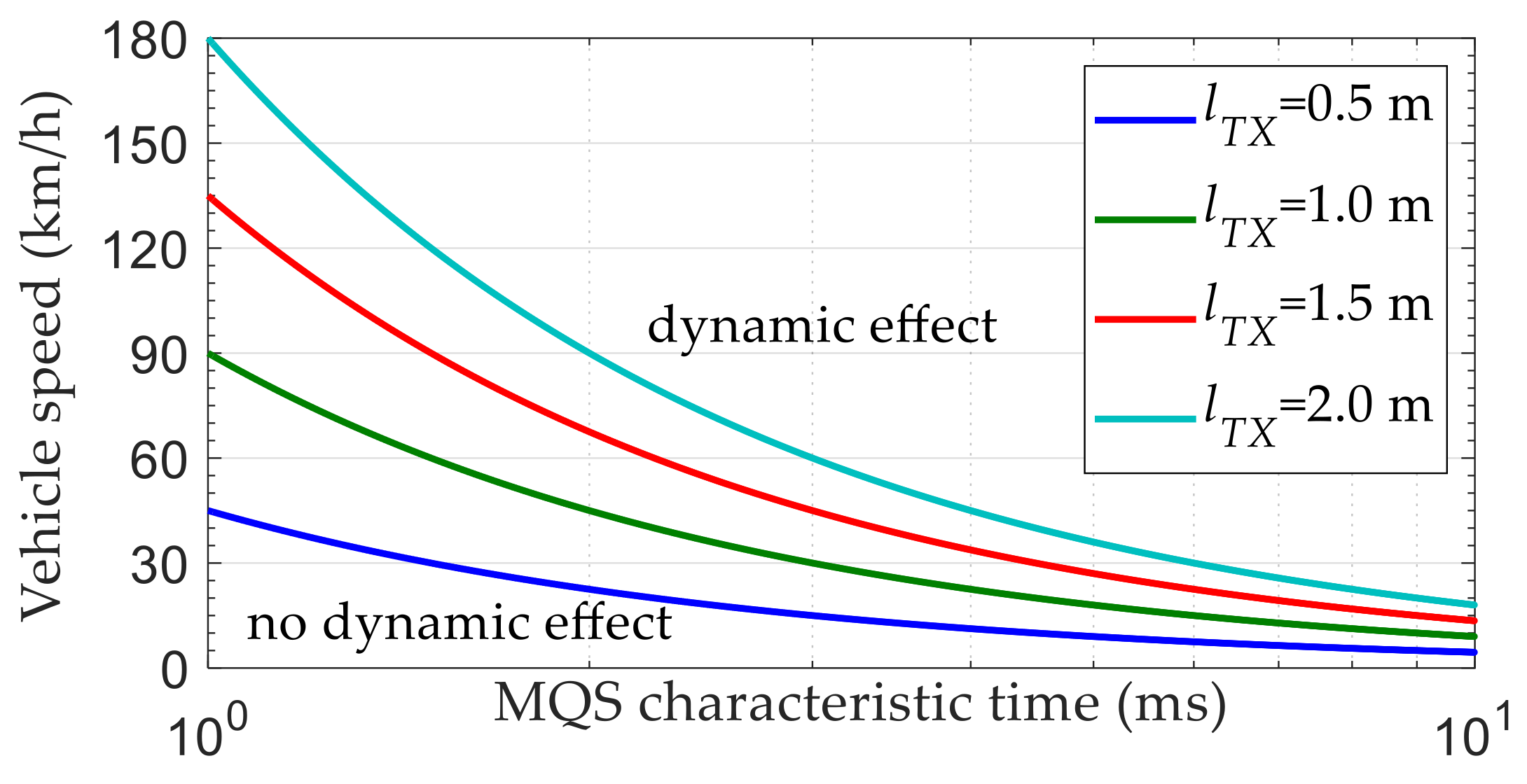In fact, its operating frequencies are of the order of kHz and the lengths l_TX are about meters, hence any reasonable vehicle speed satisfies (2). Therefore, for the purposes of this paper only (1) applies. For typical automotive WPTSs, the inductance values range from tens to hundreds of µH, and the resistances from tens to hundreds of mΩ, hence τ_M ranges from fractions to some tens of ms. Assuming δ = 0.1 in (1), we can compute the maximum vehicle speed values above which the dynamic effects must be taken into account (see Figure 1).

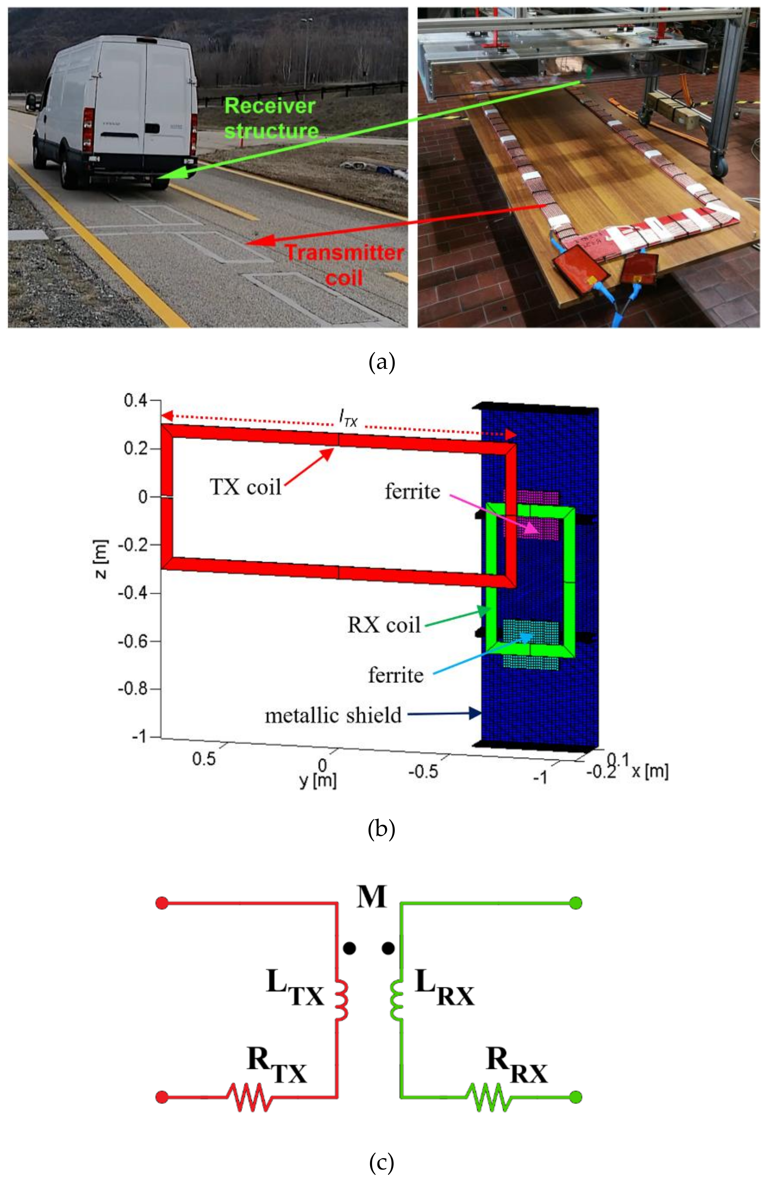
The dynamic WPTS depicted in Figure 2 has been adopted as case study in this paper. It has been used as benchmark in the H2020-EMPIR project “Metrology for Inductive Charging of Electric Vehicles (MICEV)” [27,28]. Full details on the system are provided in [29]. The TX and RX coils are shown in Figure 2b. They have both 10 turns with 28 mm² cross-section and 5-mm thickness. The inner size is 150 cm × 50 cm for the TX coil and 30 cm × 50 cm for the RX coil. The RX coil is installed on board the EV into an aluminum case. Two ferrite blocks with relative permeability μ_r = 2000 are used to improve the magnetic coupling. 50 TX coils are embedded in the road pavement, making a 100 m long charging lane. The nominal vertical distance between the RX coil and the TX coils is 20 cm. The chassis conductivity is 33.4 MS/m. The system can transfer 11 kW maximum power at 85 kHz frequency [30].

In order to verify criterion (1), a numerical electrodynamic simulation of the system has been carried out by means of the full 3D commercial solver ANSYS Maxwell [31], on a simplified system made by a TX and RX coil with only one turn, with inner lengths l_TX = 1.5 m and l_RX = 0.3 m, at a frequency of 85 kHz. In the nominal position, where the centers of the TX and RX coils are aligned along the same vertical axis, the quasi-static parameters of coils are given by: R_TX = 30 mΩ, R_RX = 15 mΩ, L_TX = 80 µH, L_RX = 10 µH and M = 8.51 µH. From these values, it is τ_M = 2.7 ms. According to (1), the maximum vehicle speed should be v₀ ≈ 50 km/h. An electrodynamic model was built in ANSYS Maxwell, imposing the motion of the RX coil along the longitudinal axis of the TX coil, with a constant speed of 36 km/h (10 m/s). The values of M_D computed at given time instants (corresponding to different longitudinal position of the RX coil) are reported in

Table 1. ComputeTd dynamic and static values of mutual inductance.

Time Instant (ms)	MD (µH)	MS (µH)	Error (%)
0	−1.45	−1.41	2.76
10	0.54	0.55	1.85
20	3.39	3.21	5.31
30	5.99	6.30	5.17
48	8.60	8.51	1.05

, along with the values of M_S computed under the static limit in the positions corresponding to the same time instants. At the initial position (t = 0 ms), the RX coil is completely outside the TX one, whereas at the final position (t = 48 ms), the RX coil is completely inside the TX one and their axes are perfectly aligned (nominal position). The two solutions differ by a maximum relative error of about 5–6%, hence demonstrating the validity of the criterion (1). Of course, lower values of δ in (1) would provide a better accuracy.

3. Efficiency of Wireless Power Transfer Systems

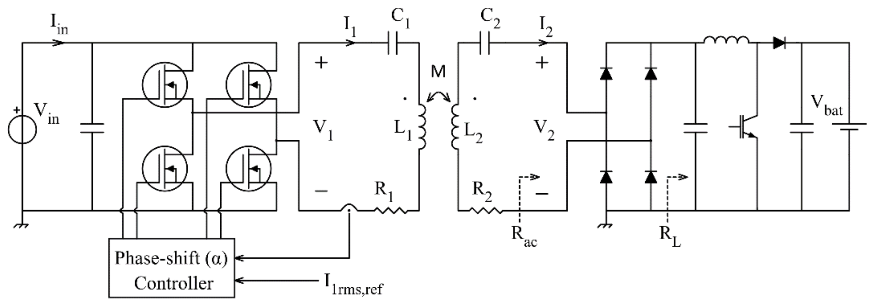
The schematic of the WPTS analyzed in this paper is shown in Figure 3. Such a series–series compensation architecture is quite general and is herein adopted as a case study to validate the proposed mutual inductance analytical behavioral model. The optimal design of both the power conversion stages and the resonant compensation architectures is out of the scope of this paper.

The inductances L₁ and L₂ of the TX and RX coils are compensated by the capacitors C₁ and C₂. The resistor R₁ includes the resistances of the L₁-C₁ series and of the two inverter MOSFETs conducting simultaneously. Similarly, the resistor R₂ includes the resistances of the L₂-C₂ series and of the two rectifier diodes. From Figure 2c and Figure 3, we have L₁ = L_TX, L₂ = L_RX, R₁ = R_TX and R₂ = R_RX. The diode-bridge rectifier at the receiver side is connected to the load (battery) through a boost converter, which regulates the equivalent load resistance R_L at the boost input to a given optimal value ensuring the maximum power transfer at the nominal mutual inductance M_nom. The inverter switching frequency f_s is equal to the resonance frequency $f_0=1/(2\mathsf{\pi }\sqrt{L_1{C}_1})=1/(2\mathsf{\pi }\sqrt{L_2{C}_2})$ of the WPTS. The full-bridge inverter at the transmitter side adopts a phase-shift control, which modulates the phase-shift angle α between the complementary square-wave gate signal pairs driving the inverter MOSFETs. The goal of the phase-shift control is to achieve a regulation of the transmitter rms current I_1rms at the desired value I_1rms,ref.

Table 2. WPTS operating parameters and component values.

fs [kHz]	Vin [V]	I1rms,ref [A]	RL [Ω]	L1 [μH]	L2 [μH]	C1 [nF]	C2 [nF]	R1 [Ω]	R2 [Ω]
85	500	28.5	8	281.4	119.8	12.5	29.2	1.157	0.555

lists the operating parameters and component values of the analyzed WPTS. Additional details on the power control in dynamic conditions and power demand regulation are available in [29,30].

At resonance we have:

$${\overline{V}}_1=R_1{\overline{I}}_1-{\mathrm{j}\mathsf{\omega }}_{0}M{\overline{I}}_2$$

(3)

$${\overline{V}}_2=R_{ac}{\overline{I}}_2={\mathrm{j}\mathsf{\omega }}_{0}M{\overline{I}}_1-R_2{\overline{I}}_2$$

(4)

where ${\overline{V}}_1$ and ${\overline{V}}_2$ are the phasors of the voltage at the transmitting and receiving coils, ${\overline{I}}_1$ and ${\overline{I}}_2$ are the phasors of the current at the transmitting and receiving coils (see Figure 3), and R_ac is the equivalent resistance seen at the diode rectifier input, given by

$$R_{ac}=\frac{V_2}{I_2}=\frac{8}{{\mathsf{\pi }}^2}{R}_L$$

(5)

Solving (3) and (4) yields (6) and (7):

$${\overline{V}}_1=\left[R_1+\frac{{\left({\mathsf{\omega }}_{0}M\right)}^2}{R_2+R_{ac}}\right]{\overline{I}}_1$$

(6)

$${\overline{I}}_2=\frac{\mathrm{j}{\mathsf{\omega }}_{0}M}{R_2+R_{ac}}{\overline{I}}_1$$

(7)

The primary and the secondary side average power P₁ and P₂, and the resulting efficiency η = P₂/P₁, are given by (8) and (9):

$$P_1=\frac{1}{2}\left[R_1+\frac{{\left({\mathsf{\omega }}_{0}M\right)}^2}{R_2+R_{ac}}\right]I_1^2,\hspace{1em}\hspace{1em}{P}_2=\frac{1}{2}\frac{R_{ac}{\left({\mathsf{\omega }}_{0}M\right)}^2}{{\left(R_2+R_{ac}\right)}^2}{I}_1^2$$

(8)

$$\eta =\frac{{\left({\mathsf{\omega }}_{0}M\right)}^2{R}_{ac}}{\left[{\left({\mathsf{\omega }}_{0}M\right)}^2+R_1\left(R_2+R_{ac}\right)\right]\left(R_2+R_{ac}\right)}$$

(9)

where the TX coil current magnitude I₁ is fixed by the inverter phase-shift control, i.e., I₁ = $\sqrt{2}$I_1rms,ref. Equation (9) highlights the impact of mutual inductance M on the WPTS efficiency. In particular, (9) shows that the efficiency increases with higher mutual inductance.

4. Mutual Inductance Behavioral Modeling for WPTS Dynamic Charging

Based on (9), two different investigations are of interest in the WPTS performance analysis in dynamic charging: (a) to analyze the WPTS efficiency over a given trajectory, and (b) to identify a trajectory, or a trajectory bound, ensuring a certain efficiency target. In both cases, a function providing mutual inductance M is needed. The generation of the analytical behavioral model of mutual inductance for the case study WPTS of Figure 2 and Figure 3 has been discussed in [32]. A key concept in the generation of behavioral models for the coils of a WPTS is the proper selection of the range of conditions for which the model is expected to provide a reliable prediction of mutual inductance. This allows for a proper restriction of the minimal input data set needed to the algorithm that generates the model. In this regard, for the case under study, it is important to consider only the trajectories of real-world interest.

Figure 4 shows some trajectories of the RX coil while the EV transits over two subsequent TX coils along the y-axis. Two TX coils only are considered in this example for clarity. Nevertheless, the discussion can be easily extended to all the 50 TX coils of the charging lane.

The ideal trajectory ensuring the maximum efficiency is the one shown in Figure 4a, with the RX coil moving along the y-axis with Δz = 0 cm. Indeed, in this case the mutual inductance is maximum. In reality, an EV may likely follow a trajectory that is affected by a constant lateral displacement Δz ≠ 0 during the transit across the charging lane, as shown in Figure 4b (case #1), or by a varying lateral displacement Δz(y) ≠ 0, as shown in Figure 4c (case #2). Accordingly, the two cases of Figure 4b,c are considered to provide the data for the model generation algorithm. Each trajectory is discretized by a sequence of sampled positions, described by the displacements (Δy, Δz) of the RX central point with respect to the axis origin (y₀ = 0, z₀ = 0), corresponding to the center of the left-side TX coil.

The values of (Δy, Δz) considered for the aforesaid case studies are listed in

Table 3. RX coil misalignment conditions.

[cm]	Case #1
Δy	{0, 23.4, 35.0, 46.8, 55.0, 70.1, 93.5, 116.9, 140.3, 163.6, 187.0, 210.4}
Δz	{0, 6, 12, 18, 24, 30}
[cm]	Case #2
Δy	−80.2	−39	2.2	43.4	84.6	125.8	167	208.2	249.4	290.6
Δz	−30.2	−26.8	−23.5	−20.1	−16.8	−13.4	−10.1	−6.7	−3.4	0

.

The six values of Δz considered for case #1 combined with the 12 values of Δy provide 72 positions, which define the Training Data Set (TDS) of the behavioral model generation algorithm [32]. The 10 positions of case #2, instead, are used as a Validation Data Set (VDS) for the resulting behavioral model. The values of the mutual inductance between the TX and RX coils for all the 72 TDS and 10 VDS positions have been calculated under MQS limits by means of the FEM electromagnetic solver Cariddi [33]. To ensure discretization errors below 1%, the mesh was assessed to 49,728 elements and 69,076 nodes. The simulation time for each point is 7878 s (about 131 min), on a 25 cores system (Intel(R) Xeon(R) CPU E5-4610 v2 @ 2.30 GHz). For a single TX–RX coil pair,

Table 4. Self and mutual inductances of the WPTS coil pair.

Parameter	FEM Simulation	Experimental Values
LTX (µH)	278.6	281.4
LRX (µH)	115.4	119.8
M (µH)	18.1	18.3

shows the comparison between the simulated values of mutual and self-inductances and the measured values in the nominal position, thus confirming the reliability of the adopted numerical tool. The resistance values measured for the WPTS under study are R_TX = 359 mΩ and R_RX = 128 mΩ. Accordingly, the largest time constant of the MQS problem is estimated in 0.94 ms. On the other side, the RX coil requires about 133 ms to cover the distance of 3.7 m over the two TX coils at a constant speed of 100 km/h. In practical cases, this time is much longer than the MQS time constant. Consequently, any dynamic effect can be neglected in the mutual inductance evaluation, allowing us to consider the case studies in Table 3 under static limit.

As discussed in [32], it is sufficient to identify the behavioral model for a single RX–TX coil pair, M_tx1,bhv (Δy, Δz), between the RX coil and the left side TX coil of Figure 4, and use such a model to evaluate the total mutual inductance M_tot, given in (10):

$$M_{tot}=M_{tx1,bhv}\left(\Delta y,\Delta z\right)+M_{tx1,bhv}\left(\Delta y-2\Delta y_{mid},\Delta z\right)$$

(10)

where the second term represents M_tx2, i.e., the mutual inductance between the RX coil and the right side TX coil, while Δy_mid = 1.052 m is the middle point between the two TX coils. In addition, as M_tx1 is symmetric with respect to the left side TX coil center, the TDS of case # 1 can be increased up to 138 points, by mirroring the M_tx1 values obtained for positive Δy values to negative symmetric Δy values.

The mutual inductance values calculated by means of Cariddi (other solvers can be used as well) over the TDS are used by a Genetic Programming Algorithm (GPA) [34], which generates analytical expressions of the mutual inductance M_tx1 = M_tx1,bhv (Δy, Δz) as a function of Δy and Δz. The details regarding the setup and execution of the GPA developed for this study are discussed in [32]. Here, we put the focus on the criteria adopted to drive the GPA in the generation of candidate functions M_tx1,bhv. In particular, a first fundamental choice concerns the discrimination between Δy and Δz, as these two geometric variables play different roles. Indeed, while Δy is associated to the vehicle movement direction, and then it is the main variable influencing the time variation of the mutual inductance, Δz is rather a bias factor, as it is associated to the EV lateral drift, which is not expected to change too much during the vehicle transit along the charging lane. For this reason, the GPA has been set up to generate functions M_tx1,bhv (Δy, p(Δz)), where the analytical structure M_tx1,bhv is determined by the way M_tx1 changes along Δy, and the coefficients p are functions of Δz and are determined by the way M_tx1 changes along Δz. This separation of variables greatly helps in keeping the behavioral model simple and suitable for the application purpose. Among the best candidate models generated by the GPA discussed in [32], the following model provides a good trade-off among complexity, accuracy and repeatability:

$$M_{tx1,bhv}=p_0\tanh \left[p_1(\Delta y^2+p_2)\right]+p_3\mathrm{atan}(|p_4\Delta y{|}^{p_5})+p_6$$

(11)

where Δy and M_tx1,bhv are expressed in meters and μH, respectively. The model given in (11) is characterized by high repeatability over GPA runs and small error on the TDS and VDS. The coefficients p_k (k = 0, 1, …,6) have a regular and monotonous trend, and can be analytical represented by arctangent functions of Δz (in meters):

$$p_k=a_{k,0}\mathrm{atan}(a_{k,1}(|\Delta z|-a_{k,2}))+a_{k,3}$$

(12)

The values of the fitting coefficients {a_k,0, a_k,1, a_k,2, a_k,3} are listed in

Table 5. Coefficient values for the behavioral model given in (11).

Coefficients	ak,0	ak,1	ak,2	ak,3
p0	13.3	7.35	0.190	−17.7
p1	0.136	20.2	0.257	2.93
p2	−0.05	8.40	0.234	−0.484
p3	9.92	7.32	0.187	−14.0
p4	0.12	8.46	0.263	−1.5
p5	1.08	7.28	0.323	−2.73
p6	−13.2	7.40	0.189	17.9

.

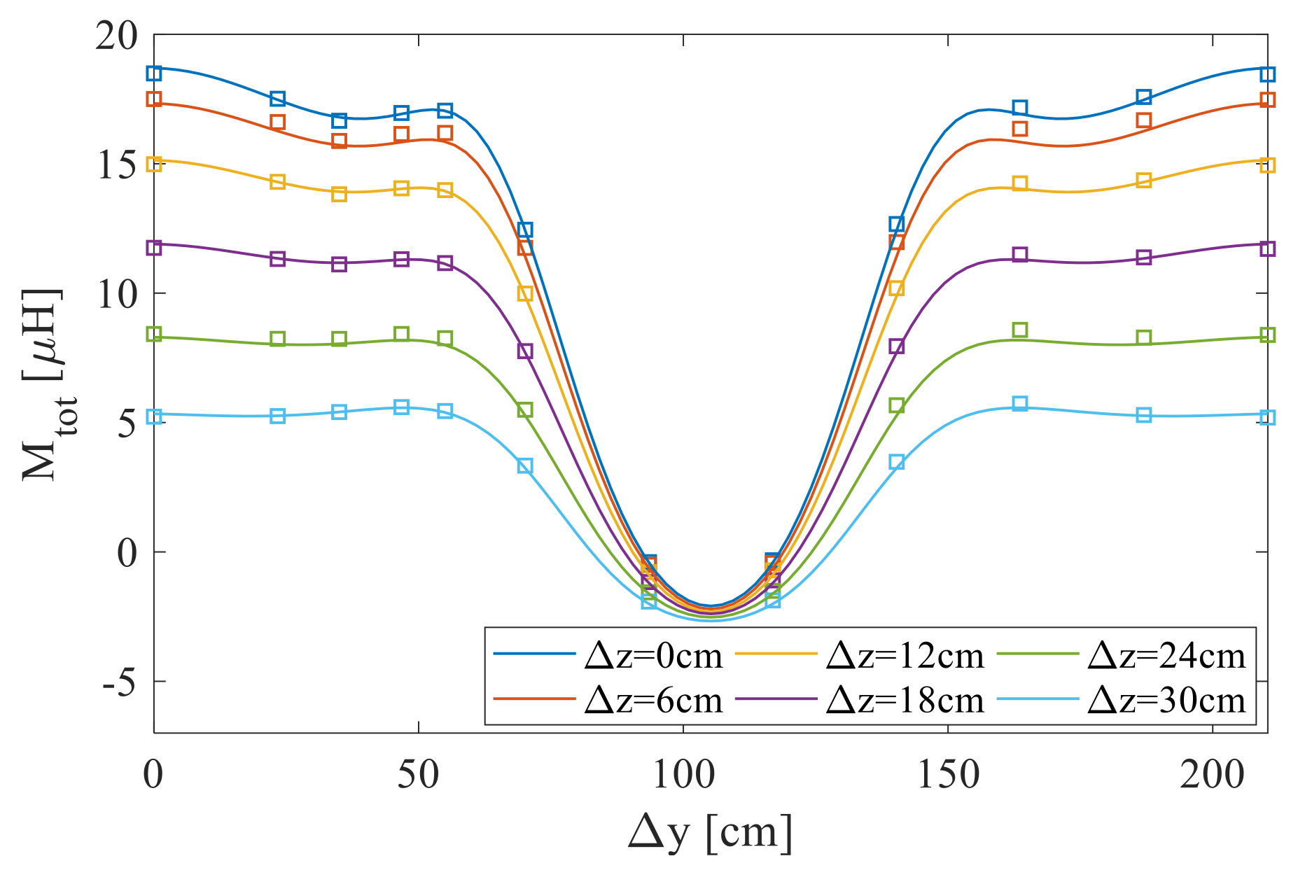
The plots of Figure 5 show the total mutual inductance M_tot obtained by combining the formulas given in Equations (10)–(12), for the TDS trajectories of case #1.

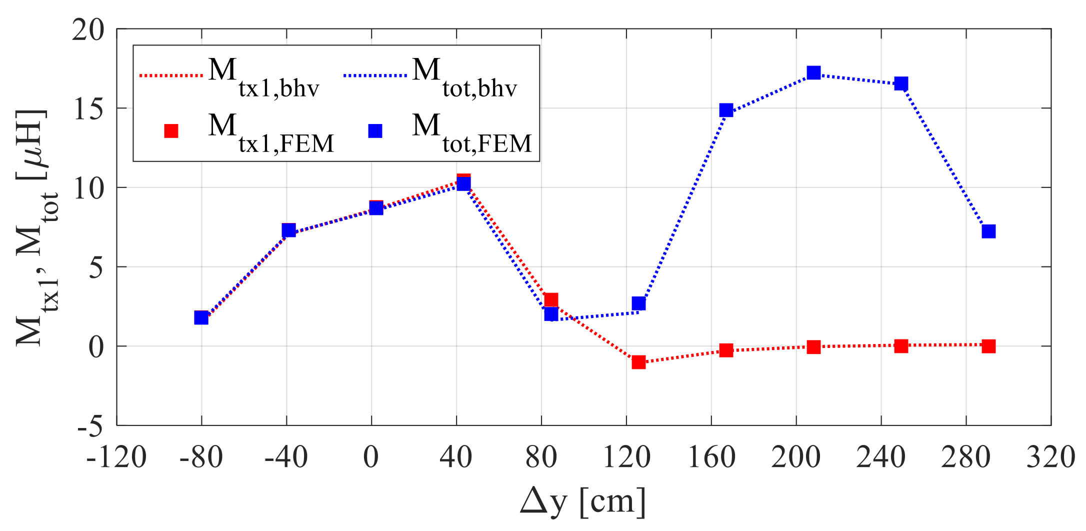
Figure 6 compares the predictions of M_tx1,bhv and M_tot,bhv (dotted lines) to the corresponding FEM-based data (square markers), for the case #2 VDS trajectory. The plots of Figure 5 and Figure 6 confirm the good accuracy and the generalization capability of the behavioral model given in Equations (10)–(12).

5. Behavioral Model Experimental Validation

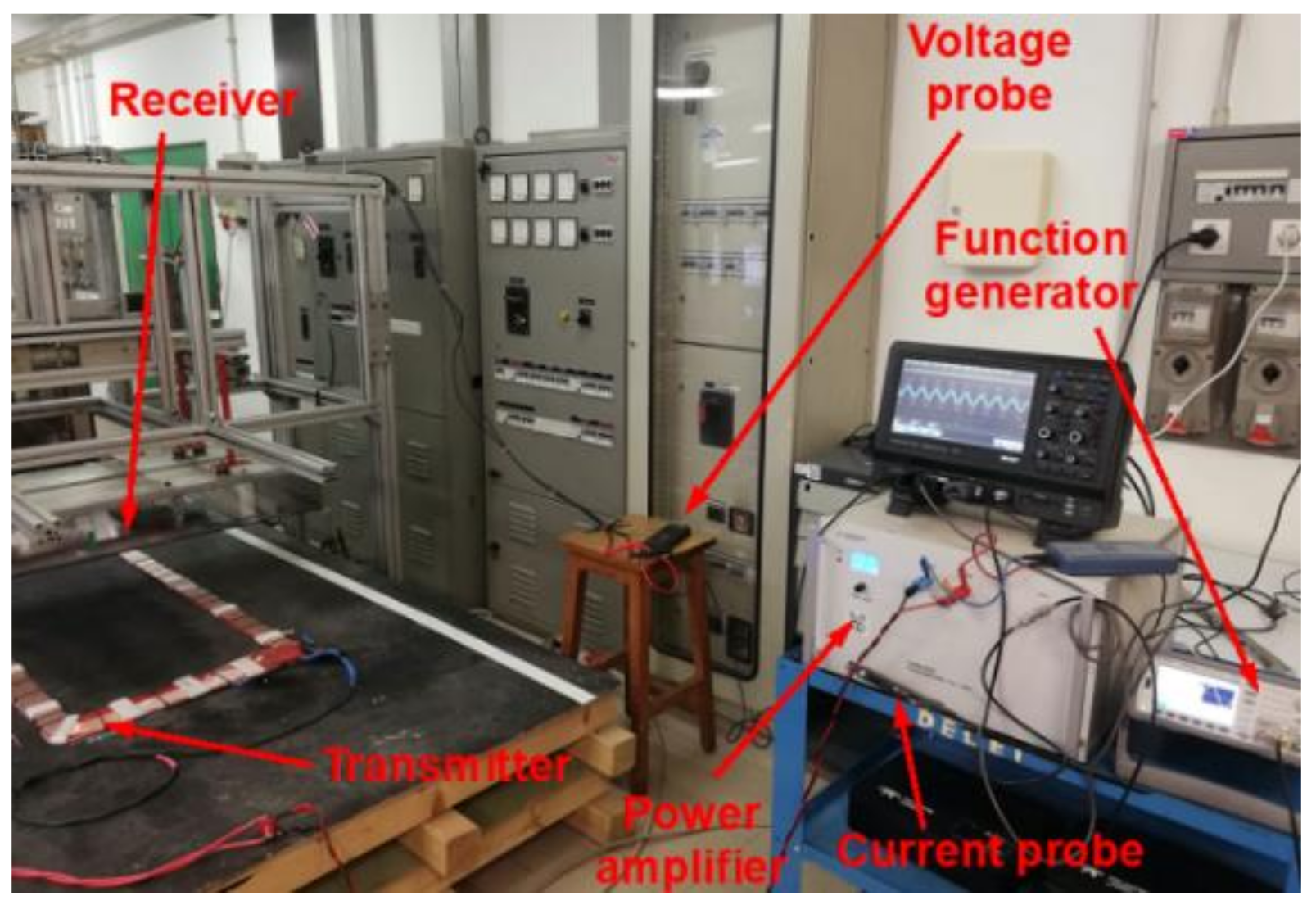
The predictions of the proposed behavioral model have been validated by means of experimental measurements performed by using two TX coils of the case study WPTS, placed at a distance of 50 cm from each other, and one RX coil moving at a nominal vertical distance of 20 cm with respect to the TX coils. The test setup is shown in Figure 7.

Each transmitter is supplied by means of a power amplifier providing a sinusoidal voltage, at the fixed frequency of 85 kHz, whose amplitude is regulated in order to supply the coil with a sinusoidal current of constant amplitude I_TX = 28.5 A. The RX coil is mounted within a movable mechanical framework that provides the possibility of fine-tuning the receiver structure position along the three axes by means of tuning screws. 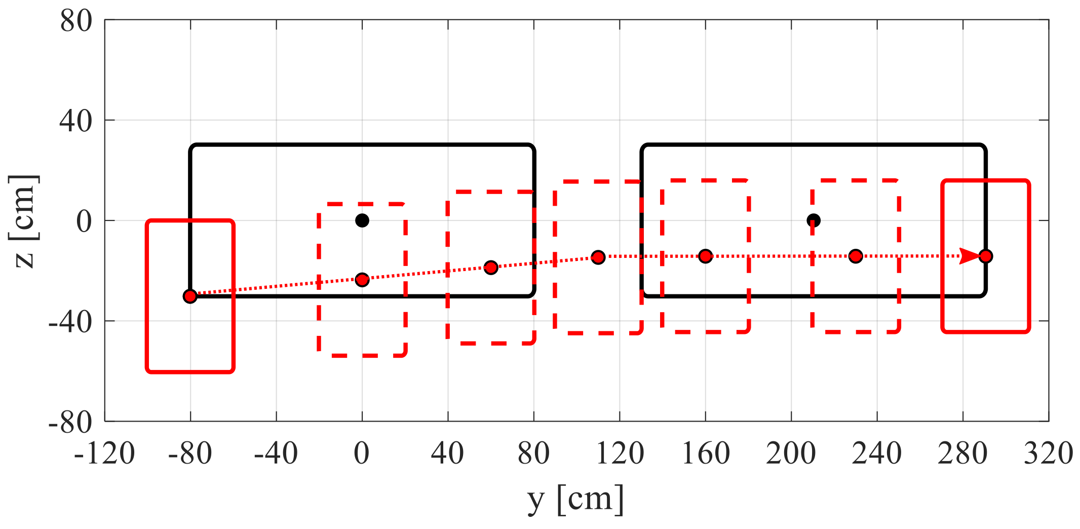The trajectory shown in Figure 8 has been considered for the test (case #3).

The values (Δy, Δz) listed in

Table 6. RX coil misalignment conditions used for the behavioral model validation.

[cm]	Case #3
Δy	−80.2	0	60	110	160	230	291
Δz	−30.2	−23.7	−18.8	−14.7	−14.7	−14.7	−14.7

correspond to the RX–TX coil reciprocal positions considered for the test (red circles in Figure 8).

The mutual inductance M is experimentally evaluated by measuring the open-circuit voltage V_OC at the receiver coil terminals by means of a differential voltage probe, according to (13):

$$M=\frac{1}{2\pi f_0}\frac{V_{OC}}{I_{TX}}$$

(13)

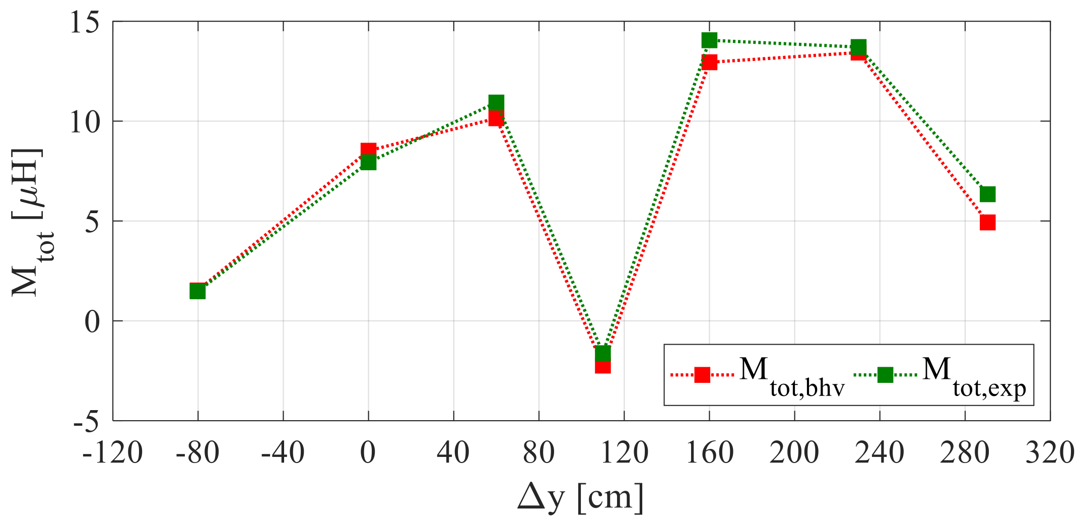
Figure 9 shows the behavioral model predictions (red square markers) of the total mutual inductance M_tot,bhv obtained by using the model given in Equations (10)–(12), compared to the experimental measured values M_tot,exp (green square markers). These results further validate the proposed behavioral model and confirm its good accuracy and generalization capability.

The proposed modeling approach can be extremely helpful in dynamic WPTS simulations, for different receiver trajectories covering a wide range of misalignment conditions. In principle, the proposed behavioral model can be applied to a WPTS composed of a number of identical TX coils, by separately evaluating their individual mutual inductances and summing their relative contributions, as was done herein for two TX coils.

6. WPTS Performance Sensitivity Analysis

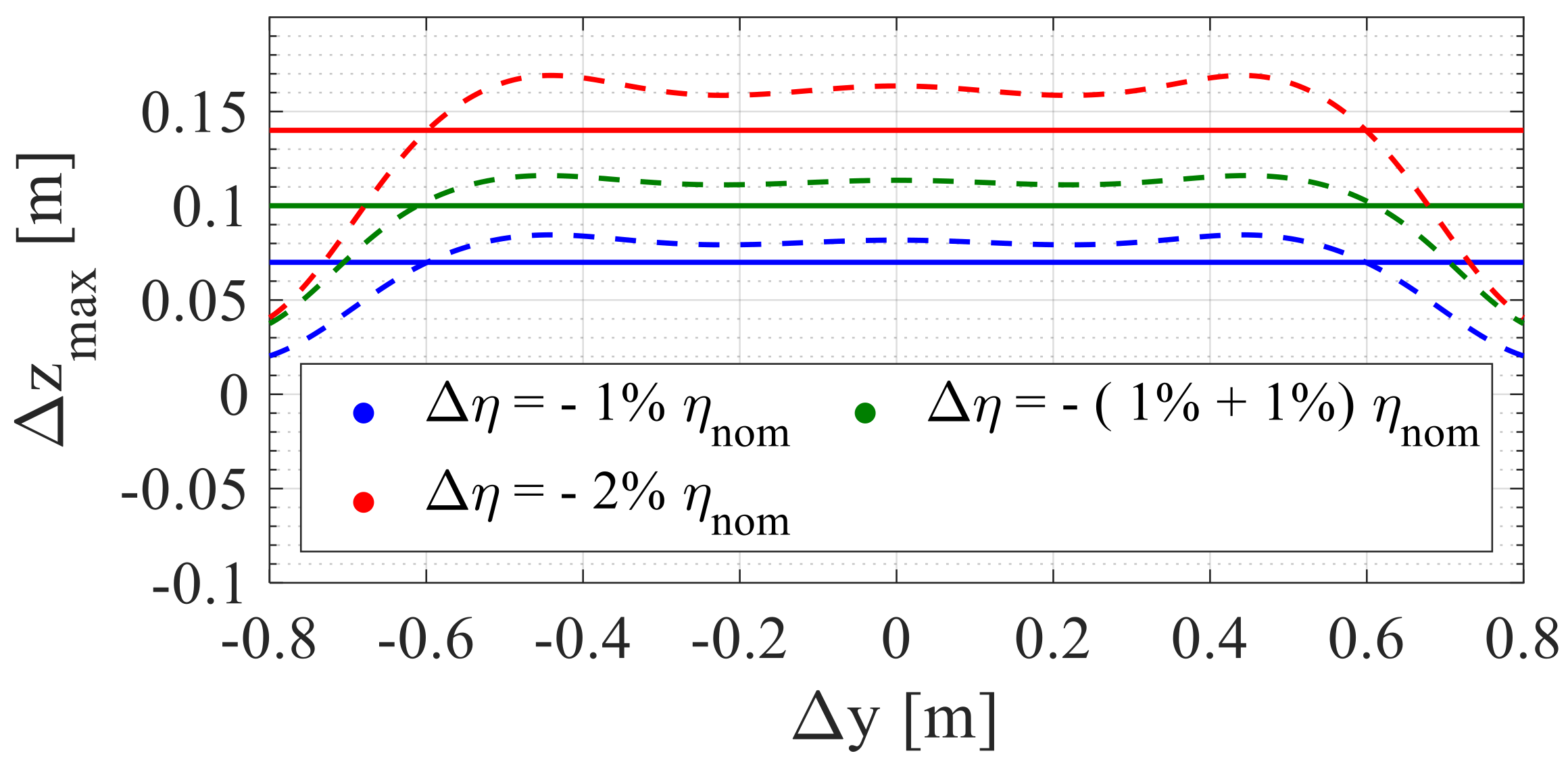
The behavioral model given in Equations (10)–(12) can be effectively used to facilitate and speed up investigations on the WPTS performance concerning the energy transfer during the vehicle transit. A key point is that no vehicle driver will be able to ensure that the vehicle exactly tracks the maximum efficiency trajectory along the symmetry axis of the TX coils. Even in case of assisted driving, the positioning systems will have a given accuracy, not ensuring perfect alignment. Let us then consider the problem of predicting the WPTS efficiency de-rating determined by the lateral drift Δz of the vehicle transiting over the charging lane. In particular, let us suppose that we want to know the maximum allowed lateral drift Δz_max ensuring an efficiency de-rating no greater than a given drop Δη, compared to the nominal efficiency η_nom achieved when the vehicle trajectory coincides with the TX coils symmetry axis. As the efficiency is function of M according to (9), the proposed behavioral model allows calculating the derivative of the efficiency with respect to Δz. By using the first-order linear approximation (14), it is possible to obtain the function Δz_max(Δy) given in (15):

$$\eta (\Delta y,\Delta z_{\max })=\eta (\Delta y,0)+\Delta \eta ,\hspace{1em}\hspace{1em}\hspace{1em}\hspace{1em}\hspace{1em}\mathrm{where} \Delta \eta \cong {\left.\frac{\partial \eta (\Delta y,\Delta z)}{\partial \Delta z}\right|}_{\Delta z=0}\Delta z_{\max }(\Delta y)$$

(14)

$$\Delta z_{\max }\left(\Delta y\right)=\frac{\Delta \eta }{{\displaystyle \sum _{k=0}^N\frac{\partial \eta (\Delta y,\Delta z)}{\partial p_k}{\left.\frac{d{p}_k}{d\Delta z}\right|}_{\Delta z=0}}}$$

(15)

Figure 10 shows the plots of Δz_max(Δy) for Δη = −1% (blue dashed line) and Δη = −2% (red dashed line) efficiency drops. The green dashed line represents the plot of Δz_max(Δy) for the −(1% + 1%) nested efficiency drop, calculated by determining the derivative of the efficiency with respect to Δz along the Δz_max(Δy) corresponding to −1% efficiency drop, and then determining the new Δz_max(Δy) curve corresponding to a further −1% efficiency drop.

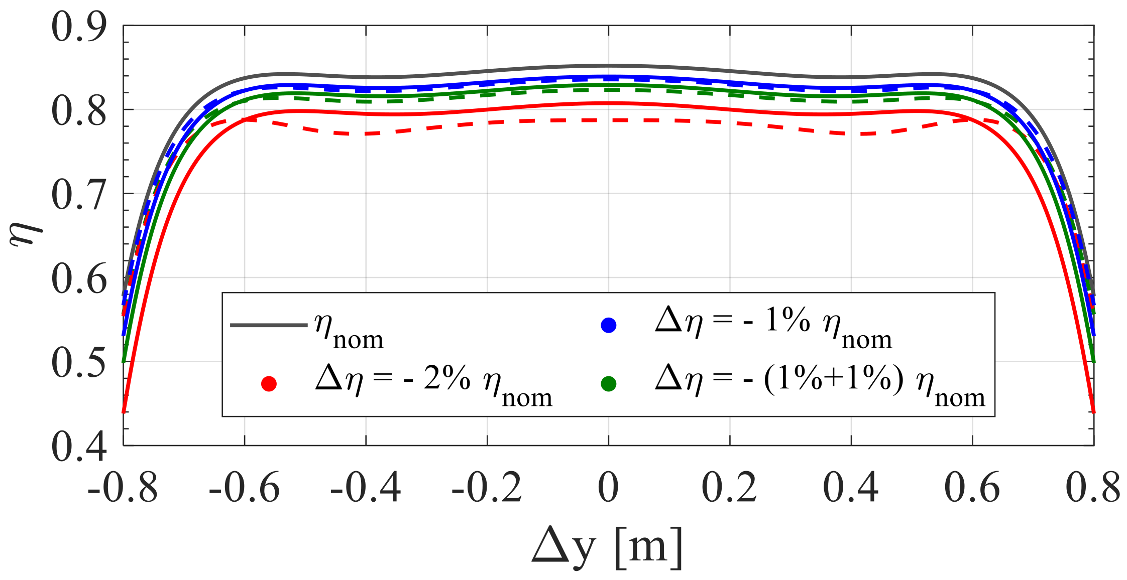
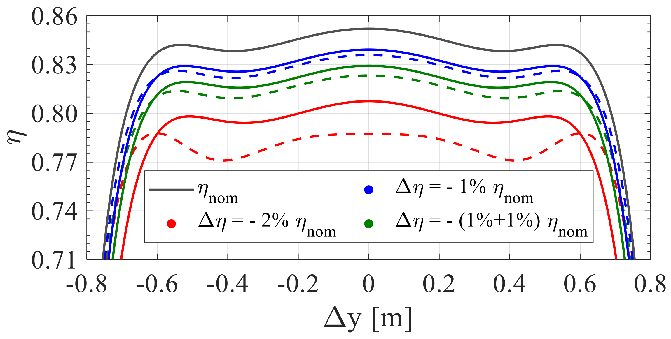
As vehicles realistically transit over each TX coil of the charging lane with an almost constant drift Δz, let us consider the average Δz_av of Δz_max(Δy) over the Δy range (solid lines in Figure 10), resulting in average lateral drifts of about 7 cm for −1%, 10 cm for −(1% + 1%) and 14 cm for −2% efficiency drop. The efficiency plots in Figure 11 and Figure 12 are calculated using the formula (9) and the model given in Equations (10)–(12) over the Δz_max(Δy) trajectories (dashed lines) and over the Δz_av trajectories (solid lines).

The plots show that a vehicle can transit with about 7 cm average lateral drift causing no more than −1% efficiency drop, and with about 10 cm lateral drift causing no more than −2% efficiency drop. Evidently, the simplified sensitivity analysis based on the proposed behavioral model is quite reliable for 1% steps, as proved by the much better prediction obtained with the nested −(1% + 1%) sensitivity analysis compared with the direct −2% sensitivity analysis, which is not much reliable. A similar sensitivity analysis of the WPTS power performance as a function of vehicle trajectory can be performed using the proposed behavioral model and the Formula (8).

7. Conclusions

This paper discusses the behavioral modeling of the mutual inductance between coupled coil pair used in dynamic charging Wireless Power Transfer Systems (WPTSs). A multi-objective Genetic Programming Algorithm (GPA) has been used to generate analytical expressions of mutual inductance between TX and RX coils as a function of the misalignment parameters of interest relevant to realistic vehicle trajectories. The mutual inductance values predicted by using such behavioral model are in excellent agreement with the Finite Element Method (FEM)-based simulations and the experimental measurements, thus confirming the model accuracy and generalization capability. The mutual inductance behavioral model enables the sensitivity analysis of the WPTS power and efficiency performances with respect the vehicle misalignment during the dynamic charging process. Moreover, the adoption of behavioral models of mutual inductance considerably reduces the computation times in dynamic WPTS simulations, enabling system-level simulations for different receiver trajectories and over a wide range of misalignment test conditions. Indeed, for fast yet reliable simulations, the final user can easily implement in any commercial simulator the analytical expressions of mutual inductance, given as a function of the misalignment parameters of interest. As prospective work, the behavioral modeling of mutual inductance in dynamic charging applications can be of huge interest in the optimal design and parametric optimization of dynamic WPTSs.