Robust Data-Driven Soft Sensors for Online Monitoring of Volatile Fatty Acids in Anaerobic Digestion Processes


1
Departament d’Enginyeria Química, Universitat Rovira i Virgili, Avda. Paisos Catalans, 26, 43007 Tarragona, Spain
2
LBE, Univ Montpellier, INRA, 102 Avenue des Etangs, 11100 Narbonne, France
*
Author to whom correspondence should be addressed.
Processes 2020, 8(1), 67; https://doi.org/10.3390/pr8010067
Submission received: 12 November 2019
/
Revised: 12 December 2019
/
Accepted: 31 December 2019
/
Published: 3 January 2020
(This article belongs to the Section Chemical Processes and Systems)
Abstract
:The concentration of volatile fatty acids (VFAs) is one of the most important measurements for evaluating the performance of anaerobic digestion (AD) processes. In real-time applications, VFAs can be measured by dedicated sensors, which are still currently expensive and very sensitive to harsh environmental conditions. Moreover, sensors usually have a delay that is undesirable for real-time monitoring. Due to these problems, data-driven soft sensors are very attractive alternatives. This study proposes different data-driven methods for estimating reliable VFA values. We evaluated random forest (RF), artificial neural network (ANN), extreme learning machine (ELM), support vector machine (SVM) and genetic programming (GP) based on synthetic data obtained from the international water association (IWA) Benchmark Simulation Model No. 2 (BSM2). The organic load to the AD in BSM2 was modified to simulate the behavior of an anaerobic co-digestion process. The prediction and generalization performances of the different models were also compared. This comparison showed that the GP soft sensor is more precise than the other soft sensors. In addition, the model robustness was assessed to determine the performance of each model under different process states. It is also shown that, in addition to their robustness, GP soft sensors are easy to implement and provide useful insights into the process by providing explicit equations.
1. Introduction
Anaerobic digestion (AD) is a well-established process for stabilizing municipal sewage sludge and treating organic waste products and wastewaters from different industries, households and farms. In this process, the organic matter biodegrades in an oxygen-free environment. This leads to decomposition and bioconversion of organic matter into biogas, which mainly consist of CH4 (50–60%) and carbon dioxide (30–40%), with some other trace gases such as hydrogen sulfide and water vapors, etc. [1]. The methane gas produced can be used as an energy source for generating electricity and heating the AD reactor. The benefits of the AD process are high organic load treatment, low sludge production, energy is recovered when the biogas produced is used and operating costs are reduced due to the oxygen-free operation [2]. Many operational parameters affect the performance and effluent quality of the AD process; therefore, frequent monitoring of these parameters is crucial to ensure a stable performance. Among these parameters, pH, partial alkalinity and volatile fatty acids (VFAs) are the most important measurements for monitoring the stability and performance of the digesters with low buffering capacity. However, in the highly buffered digester, although the process is extremely under-stressed, the pH may vary very little; in this case, VFAs are the only reliable measurement for process monitoring. VFAs are key intermediate products for the reactions that produce CH4, while their accumulation inside the reactor inhibits the bacteria and causes a lower methane production rate so that the process fails [3]. The common VFA monitoring approach in a wastewater treatment plant is online and/or offline analysis. However, the measuring procedure is very costly and characterized by time-delayed responses that are often undesirable for real-time monitoring [4]. Moreover, due to the complex media and severe operating conditions in AD processes, the online sensors are not always reliable. This is because solid deposition, slime build-up and precipitation, among others, mean that sensors require regular maintenance and calibration. Therefore, it is imperative to develop cost-effective measuring techniques to provide the necessary information based on easily measured available variables and without installing new instruments [5]. Thanks to recent progress in measurement and instrumentation technologies, many easy to measure parameters, such as pH, temperature, flow rates, pressure and gas composition, can be measured online [6,7]. One alternative for dealing with these issues is using software sensors. Soft sensors are models that estimate a hard-to-measure property by using relatively easy measurements. Soft sensors have been successfully applied in monitoring and controlling wastewater treatment plants [4] and can be classified into three main categories: mechanistic, data-driven and hybrid models, depending on their underlying methods [8]. Hybrid modelling approaches are often preferred over more complex mechanistic approaches, such as the anaerobic digestion model (ADM1). In hybrid modelling, the known linear/non-linear behaviors of the system can be described by a mechanistic approach and the unknown relationships among variables can be defined by data-driven models. Hybrid models can be more precise than mechanistic models because they integrate two approaches [5]. Unlike hybrid models, data-driven models depend solely on a priori knowledge. The algorithm determines connections between input and output variables, and therefore it is a very attractive replacement of mechanistic models when they are not valid or available [9]. Different techniques such as multivariate statistical methods, multiple linear regression (MLR), principal component regression (PCR), partial least squares (PLS) regression, artificial neural networks (ANNs) and fuzzy systems are used to design different soft sensors for wastewater treatment processes [4,10,11].
Tay et al. [12] applied a neuro-fuzzy model to predict the response of high-rate AD based on different system disturbances. Their model inputs were organic loading rate (OLR), hydraulic loading rate (HLR), alkalinity loading rate (ALR), volumetric methane production rate (VMP), total organic carbon (TOC) and VFA (volatile fatty acid). Their model outputs were VMP, TOC and VFA prediction one hour ahead. They showed that their model can predict the response of anaerobic wastewater for treatment systems in the presence of OLR, HLR and alkalinity loading shocks.
Mullai et al. [13] studied the performance of an anaerobic hybrid reactor for treating penicillin-G wastewater. The experimental data were modelled by an adaptive network-based fuzzy inference system (ANFIS). Time and influent chemical oxygen demand (COD) were considered as inputs and effluent COD was the only output of the model. Prior to modelling, the fuzzy clustering method was used to separate the different operation phases of the digester. The R2 correlation for prediction versus actual values was found to be 0.9718, 0.9268 and 0.9796 for different phases of the digester operation. The results show that their model had a good prediction ability for COD removal efficiency. In another work, Güçlü and co-authors [14] implemented back-propagation ANN models for predicting effluent volatile solid (VS) concentration and methane yield. Effluent VS and methane yields were predicted with the ANN using pH, temperature, flowrate, VFA, alkalinity, dry matter and organic matter as model inputs. The gradient descent with an adaptive learning rate algorithm was used. The R2 correlations were 0.89 and 0.71 for VS and methane yield respectively. The authors stated that they only used conventional parameters as model inputs, which is inappropriate because VFA and alkalinity are generally not measured frequently in most real AD plants due to the above issues. Rangasamy et al. [15] studied modelling of an anaerobic tapered fluidized bed reactor for starch wastewater treatment using a multilayer perceptron neural network. ANN with two hidden layers was trained by using the back-propagation algorithm to predict different process responses, including effluent COD, biogas production, VFA, alkalinity and effluent pH. The OLR and Influent pH were considered as model inputs. Briefly, most of the studies in the past were focused on predicting VFA for a laboratory-scale anaerobic digester by using available input parameters without considering the difficulty of measuring them. Furthermore, most of the developed models were trained based on the very limited operational conditions, thus the generalization ability and performance of the models in different situations is ambiguous [14,15].
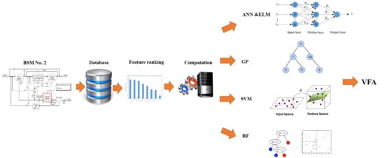
In this paper, we study the ability of different data-driven modelling techniques, such as artificial neural networks (ANNs), extreme learning machine (ELM), support vector machine (SVM), random forest (RF) and genetic programming (GP), to develop robust VFA monitoring software sensors from exclusively online easy-to-measure variables. The wrapper feature ranking method combining different models was used to select the most influential process variables for developing a data-driven soft sensor to increase the accuracy and reduce computation time. The procedure was applied to the wastewater treatment Benchmark Simulation Model No. 2 (BSM2) running in the Matlab Simulink environment. The developed software sensors were compared in terms of accuracy, robustness and transparency. Transparency is important because transparent models are very beneficial for controlling and gaining insight into the modelling procedures of AD processes. Although the Genetic Algorithm, which is very similar to the GP, has been applied for modelling AD processes, there is no soft sensor designed with the GP technique in this context [16,17]. Therefore, in this study, we discuss using the GP model for designing more transparent and interpretable soft sensors.
2. Materials and Methods
2.1. Benchmark Simulation Model No. 2
The proposed soft sensors were designed and evaluated with BSM2 [18]. The BSM2 simulation environment applies plant layout, a simulation model, influent loads, simulation procedures and evaluation criteria elements to analyze and evaluate the performances of a wastewater treatment plant. For details see Jeppsson et al. [18] for the complete layout of BSM2, which consists of a primary clarifier, an activated sludge biological reactor, a secondary clarifier, a thickener, an anaerobic digester, a dewatering unit and a storage tank. The activated sludge process consists of five reactors: two anoxic reactors with a total volume of 3000 m3 and three aerobic reactors with a total volume of 9000 m3, which are used for nitrification and predenitrification, respectively. The plant capacity has been designed for 20648 m3 d−1 of average influent with a dry weather flow rate and 592 mg L−1 of average biodegradable COD in the influent. The Activated Sludge Model No. 1 (ASM1) and the Anaerobic Digestion Model (ADM1) were used to describe the biological phenomena that take place in the activated sludge and AD reactor respectively. The influent characteristics consist of a 609 days dynamic influent data file (sampling frequency equal to a data point every 15 min) that includes rainfall and seasonal temperature variations over the year [18,19]. The first 245 days of influent data are used for plant stabilization under dynamic conditions and the last 364 days are used for the plant performance assessment.
2.2. Data Collection
The first step in designing a data-driven soft sensor is obtaining the process data. Therefore, we used synthetic data produced by BSM2. It should be noted that this paper describes a preliminary study for designing soft sensors for AD processes by applying different techniques to synthetic data; therefore, for applying the approaches discussed in this paper to real systems, real process data is necessary. Thirteen process variables obtained from the simulation are listed in Table 1. These variables are measured from the influent, effluent and gas line of AD every 15 min.
2.3. Pre-Processing of the Data
To achieve successful soft sensor development, the data set should be pre-processed to eliminate the missing and redundant values, outliers and signal noise. In this paper, as the data set is obtained synthetically from a simulator, there is no need to perform any further steps for removing the outliers and processing the missing values. However, the signal noise which is incorporated in BSM2 to obtain more comparable and realistic benchmark simulation results needs to be considered. Therefore, the signal noise should be handled appropriately for soft sensors in order to estimate VFA values accurately in different conditions. In this study, before model construction and prediction, the weighted moving average (WMA) method is adopted to reduce signal noise, as it is fast to compute and easy to use, compared to the other methods. In the WMA method each data point in the sample window is multiplied by a different weight based on its position [20] as given in Equation (1):
where Ft is the smoothed signal occurrence at time t, Wi is the weight to be given to the actual occurrence for the time t − I, Ai is the actual occurrence for the time t − i and n is the total number of window lengths in the prediction. In this work, a window length of 100 sampling times is chosen for all model constructions.
As the measured variables have different units, they need to be normalized before the different models are developed. The variable values were normalized according to their mean and standard deviation. To assess model performances, normalized root-mean-squared error (NRMSE) and the coefficient of determination (R2) were calculated according to Equations (2) and (3) respectively.
where yact and yprd are the actual and predicted values, respectively, i is the data record number, ym is average of the experimental value, and n is the total number of records.
In addition, to examine the generalization ability of the models, the overall data set is split into a training set, used to fit the model, and a validation set, used to calculate the error. In this work, the obtained simulated data from day 245 to 450 and day 451 to 609 were used as training and validation sets respectively. It should be noted that due to the high number of data points (58,465), the training set was randomly sampled and finally 1252 data points were uniformly selected to reduce the computation time during model training.
3. Data-Driven Methods
3.1. Artificial Neural Network (ANN)
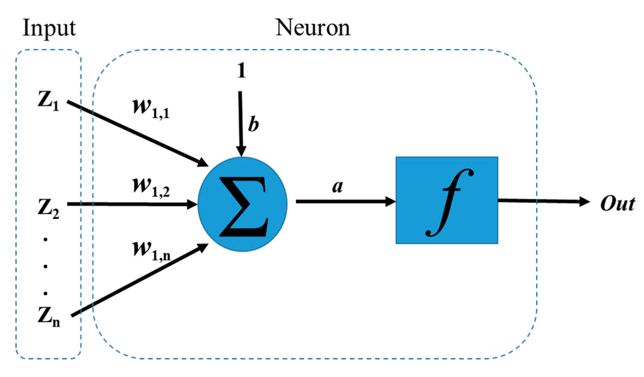
An ANN is a non-linear model that has at least three main layers, called input, hidden and output layers. All layers are connected by components called neurons (Figure 1)—in which, three main operations are carried out. First n-elements of the input vector (z1, z2, …, zn) are multiplied by weights (w1,1, w1,2, …, w1,n). Second, the weighted inputs are added together with bias signal b to obtain a value [21]:
Finally, the output signal is a function of a, the weighted sum of the inputs.
The purpose of an activation function is to ensure that the input space is mapped to a different space in the output. Linear, sigmoid and hyperbolic transfer functions are generally used in ANNs [21,22].
The structure of neurons in each layer, which are grouped and connected, is called the topology of the network. There are many different topologies; however, the Multi-Layer feedforward Perceptron (MLP) is the most commonly used. The MLP topology can be characterized by the same number of network inputs and outputs, equal to the number of input and output variables of the system to be modelled [21]. There are no specific rules for finding the best topology of the network, and therefore different methods such as trial and error or evolutionary algorithms (e.g., genetic algorithm) can be used for this purpose [23]. Once the topology is obtained, the network should be trained. We used a back-propagation algorithm using Stochastic Gradient Descent (SGD) with an adaptive learning rate algorithm [21]. There are many parameters that need to be tuned for ANN, the most important ones include the number of layers, number of neurons in each layer, type of transfer function and regularization terms (L1 and L2), which prevent overfitting and improve generalization, were considered for a grid search. The number of epochs in this work was considered to be high (2000) because the early stopping method was used. The ANN models were trained in R [24] using the H2O package [25]. To determine the best ANN structure, the number of neurons in the hidden layer was varied from 5 to 160.
3.2. Extreme Learning Machine (ELM)
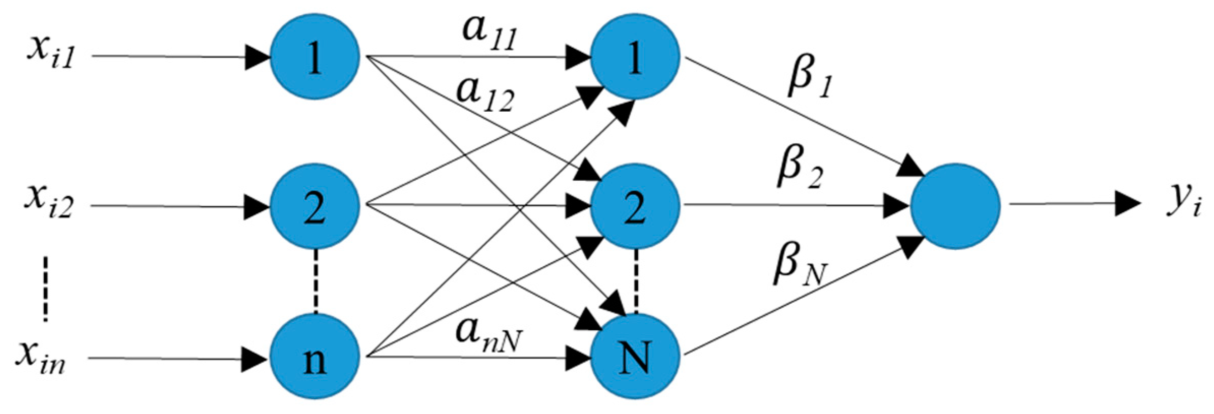
The ELM is a single hidden layer feed-forward neural network (SLFN) that was first introduced by Huang et al. [26]. In traditional ANN, all the parameters (number of neurons and hidden layers) have to be tuned, which leads to dependency between different parameters (weights and biases) in each layer. However, in ELM, the hidden layer does not need to be tuned [27]. In ELM, the input layer weights and biases are randomly initialized, then fixed without any tuning iteration. The output layer weights are calculated analytically. As there is no iterative procedure for the tuning phase, ELM has a faster learning speed than traditional ANN and has a better generalization performance. Figure 2 shows the structure of the proposed ELM model.
Considering M arbitrary distinct samples (xi, yi), where xi = [xi1, xi2, …, xin]T ∈ Rn is the input vector and yi = [yi1, yi2, …, yim]T ∈ Rm the output vector, then the output of SLFN with N hidden neurons can be calculated as:
where βj = [βj1, βj2, …, βjm] are the weights of the output layer, which need to be estimated; f(.) is the transfer function; aj and bj are the input weights and biases, respectively. Equation (5) can be written in matrix form [28]:
where, y = (y1, y2, …, yM)T, β = (β1, β2, …, βN)T and H given by:
y = Hβ
The β is determined via Moore-Penrose’s generalized inverse:
where
β = H†y
H† = (HT·H)−1·HT
The value of the input weights (aj) and biases (bj) can be randomly initialized; however, the weights of the output layer (βj) need to be determined with experimental data. Usually, the number of neurons in the hidden layer is higher than in the input layer (N > n). For the grid search, the number of neurons in the hidden layer was varied from 20 to 130.
3.3. Random Forest (RF)
The RF model was first developed by Breiman [29]. In this technique, a model is built based on a set of unpruned single regression trees. This is equal to combining different nonlinear relationships to form a more accurate non-linear model. In this method, trees are generated based on bootstrap sampling from the original training data set. In bootstrapping, random subsets of data are chosen from the original training data set to ensure the diversity among the ensemble of trees and enhance the prediction ability. The best node splitting feature for each node is selected from a set of m features that are randomly chosen from the total M features (m < M). By choosing m random features for node splitting, the correlation between different trees and thus the average response of multiple regression trees is expected to have lower variance compared to single regression trees [22,29]. RF has three main tuning parameters: the number of trees in the forest (ntrees), the number of features randomly sampled as candidates at each node split (mtry), and the maximum number of nodes in the trees (maxnode). The parameters of the RF model for the grid search were set at 2:7 (with step size 1) for mtry, and 1000 to 2000 (with step size 100) for ntrees and 5 to 30 (with step size 5) for maxnode.
3.4. Support Vector Machine (SVM)
SVM is a relatively new type of machine learning method that was introduced by Cortes and Vapnik for regression and classification problems [30,31]. The objective of SVM is to map the input vectors X onto a very high-dimensional feature space via a kernel function and then to make a linear regression in this space. The regression function can be obtained as follows [32]:
where y(x) represents predicted values, K(x, xi) is a kernel function for input features, and wi and b are coefficients. The most famous kernel functions are the polynomial kernel, the radial basis, the exponential radial basis, and the multilayer perceptron kernel function [31,33]. In this work, due to the high prediction ability, the radial basis kernel function was used. The commonly used radial basis kernel has the form:
where x and xi are support vectors satisfying the equations of kernel function K(x, xi) and is the width of the Gaussian kernel function. More information on SVM can be found in references [31,32]. To find the precise model, the tuning parameters of SVM, mainly the regularization parameter C and the inverse kernel width σ used by the radial basis kernel function, should be determined. The SVM model parameters for the grid search were set as 0.001, 0.01, 0.02, 0.1, 0.2, 0.3, 0.4, 0.5, 0.6 for , and 200 to 800 (with step size 100) for C.
3.5. Genetic Programming (GP)
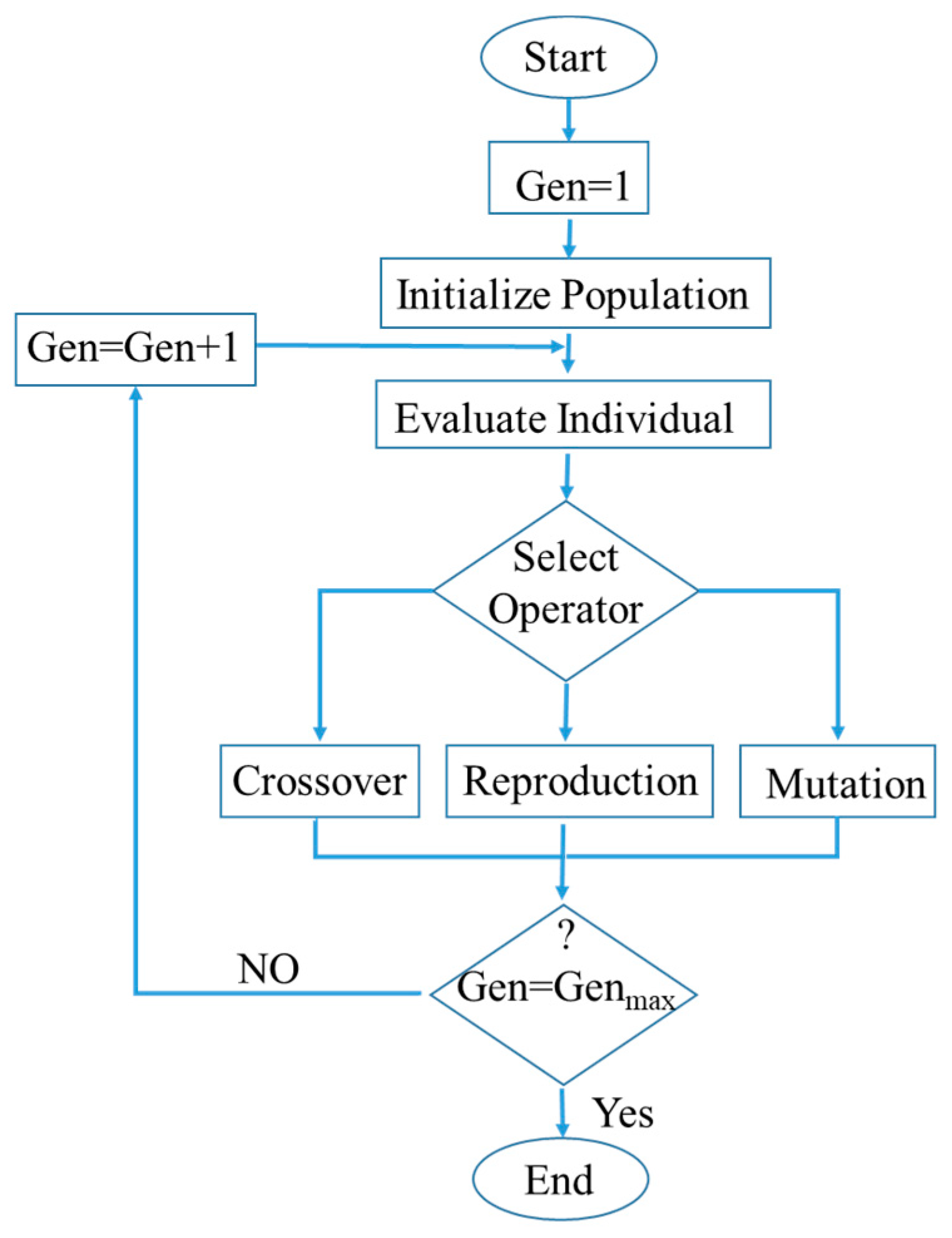
GP is a powerful method for developing a mathematical expression. It was first introduced by Koza [34]. In this method, the mathematical expressions are generated using input-output data by a biologically inspired algorithm, where the population continuously evolves towards the best-fitted model [35]. GP and the genetic algorithm (GA) have some similarities, while the most important difference is the output format. The output of GA is a value, whereas the output of GP is a computer program. The complicated structures of computer programs, mathematical expressions, and process system models in GP are represented with trees [35,36].
The GP tree structure consists of different nodes, classified into internal or external based on their position. The internal nodes can be chosen through the operators {+, −, ×, /, sin, cos, log, abs}, mathematical functions, conditional statements or even the user-defined operators. The external nodes include the constants and the model variables. After introducing data into the algorithm, the population is randomly generated. This stage is crucial to increase diversity among the models. In the next stage, each model is evaluated by a fitness function to determine how well the developed models fit the observed data. The new generation is built based on the models, having a lower fitness error. The next generation of models is reproduced by using genetic operators, such as the reproduction, crossover and mutation operators [34,35]. In the crossover operator, two models exchange the sub-trees to generate two new models, while in the mutation operator, the new model is formed from the previously generated model by substituting a randomly selected sub-tree with a newly generated one. The mutation operator is used to increase the genetic diversity of the population. The reproduction operator copies models without any change to the next generation. The fitness evaluation step is repeated for the newly generated population, and the whole procedure continues until an acceptable fitness value is achieved or the algorithm reaches its generation limit. By using this iterative procedure, the accuracy of each model improves in each iteration and finally the best one is considered as the output of the GP algorithm [34,35]. Figure 3 shows a flow chart of the GP computation procedure:
3.6. Feature Ranking
Using many features for model building can cause many problems and directly affect the model accuracy. Hence, the redundant and unnecessary features should be eliminated as they may add noise and have no impact on the dependent variable. Using feature ranking helps to determine the importance of features and reduce the dimension of the data set [37]. The other benefits of the feature ranking method are shorter training time, ease of interpreting models, overfitting reduction and lower cost in data collection. The wrapper method obtains different variable importance results depending on the feature ranking model applied. We used the fscaret package of the R environment to avoid this problem [24,38]. Briefly, variable ranking is performed in three steps: model training, variable ranking extraction, and variable ranking scaling according to the generalization error. The final variable ranking is obtained by multiplying the raw variable importance with the fraction of minimal error obtained from models by the model’s actual error according to the equation below [39]:
where weightedImpi is the weighted average of the individual model; rawImpi is the raw importance of the variable obtained from model i; minError is the minimal error obtained (RMSE or MSE) for all models; and Errori is error for model i.
4. Results and Discussion
4.1. Studying the Relationship between Input and Output Data
Before fitting non-linear models to the calibration data set, it is necessary to check whether a linear model can describe the relationships between parameters. If a linear model describes the relationships, then there is no need to use the more complicated models. Therefore, a simple linear regression (LR) was performed to predict VFA. We ran the BSM2 simulation based on the default influent file and the data signals recorded according to Table 1. As mentioned earlier, in most of the previously published studies, the authors used hard to measure parameters, such as VFA, COD, alkalinity, etc., to develop different soft sensors for the wastewater treatment processes. Therefore, in this work, the COD, alkalinity and BOD were initially eliminated from the model’s input candidate list. Due to the simplicity of the LR model, it is not necessary to perform feature ranking prior to modelling, thus the rest of the parameters according to Table 1 were used for the LR model. Next, to determine the effect of other hard to measure parameters, such as TSS and Ammonia, on the outcome, they were removed one by one from the input data of the LR model and the error was calculated. The results of the LR models with different input vectors are shown in Table 2.
The results clearly show that the relationship between parameters is highly linear. The LR model can still predict VFA with high accuracy even when TSS and Ammonia are eliminated from the input vector. This is contrary to the real behavior of the AD process, which is a very non-linear system. The most logical reasons for this linearity are the default influent data file and the design of the AD reactor itself. The default influent file is designed in such a way that the variation in the organic load to the AD reactor is not very intense, and thus, inhibition phenomena, which are the main source of non-linearity in the AD process, will not occur. In addition, the AD reactor is quite over-designed compared to its feed load, and small disturbances from the sludge recovery unit do not have a great impact on its operation. Therefore, it is possible that the process is pushed towards very narrow linear operational ranges. Thus, to increase the non-linearity and make the simulated AD process more realistic and challenging, we manipulated the feed load to the reactor. Furthermore, by manipulating the feed load, the AD’s behavior is similar to the co-digestion, which is more interesting than the mono-digestion process. We randomly changed the concentration of the inorganic nitrogen (Sin), the composite (Xc), and the carbohydrate (Xch) as well as the feed flow rate of the reactor. The summary of default and modified values of the parameters are shown in Table 3.
After manipulating the AD feed signal, a new LR model with the same approach was implemented with the new data set to determine the impact of changes on the VFA prediction. The prediction results are shown in Table 4.
It can be seen that by manipulating the AD feed carbon, inorganic nitrogen load and feed flow, the process is pushed towards the non-linear operational ranges. The best Test_NRMSE is obtained by using all inputs except ammonia concentration. Although the accuracy of this model is better than the other LR models, its performance is far from an acceptable range. Thus, there is a demand for accurate prediction of VFA by non-linear models. In the next sections of this paper, non-linear approaches are applied to the newly obtained data set to develop more accurate soft sensors.
4.2. Choosing the Most Influential Variables Using the Feature Ranking Method
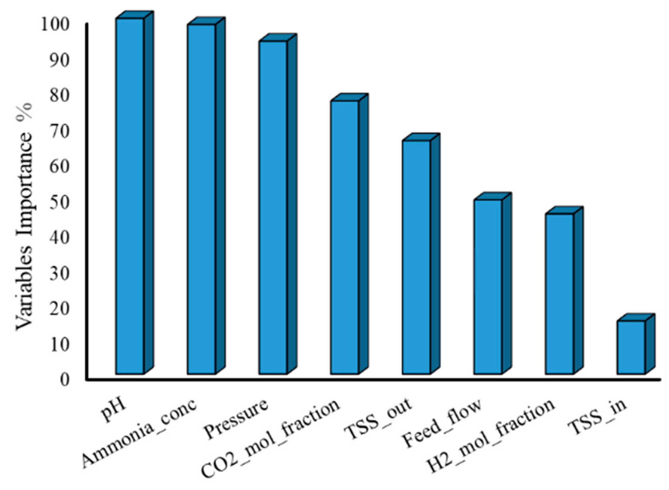
As mentioned earlier, using redundant and unnecessary features may add noise to the model and increase the risk of over-fitting. Therefore, a combination of influential sensor measurements should be chosen as model inputs. The measurements must be the most influential and, at the same time, they have to be easy to measure to satisfy the soft sensor definition. The best combination of parameters is generally chosen with feature ranking techniques. In the present study, we used the fscaret feature ranking technique. Before carrying out the feature ranking method, hard to measure parameters, including COD, alkalinity and BOD, were removed from the data set. The gas flow and CH4 mole fraction were also removed due to their direct correlation with pressure and CO2 mole fraction respectively. It should be noted that the same results could be obtained by using gas flow and CH4 mole fraction instead of using pressure and CO2 mole fraction; therefore, the decision to eliminate correlated parameters can be made based on the simplicity and availability of measurements. The remaining parameters, listed in Table 1, were used as an input vector for the fscaret method. Figure 4 shows the importance of the variables on a scale from 0 to 100 obtained with the fscaret method for VFA prediction.
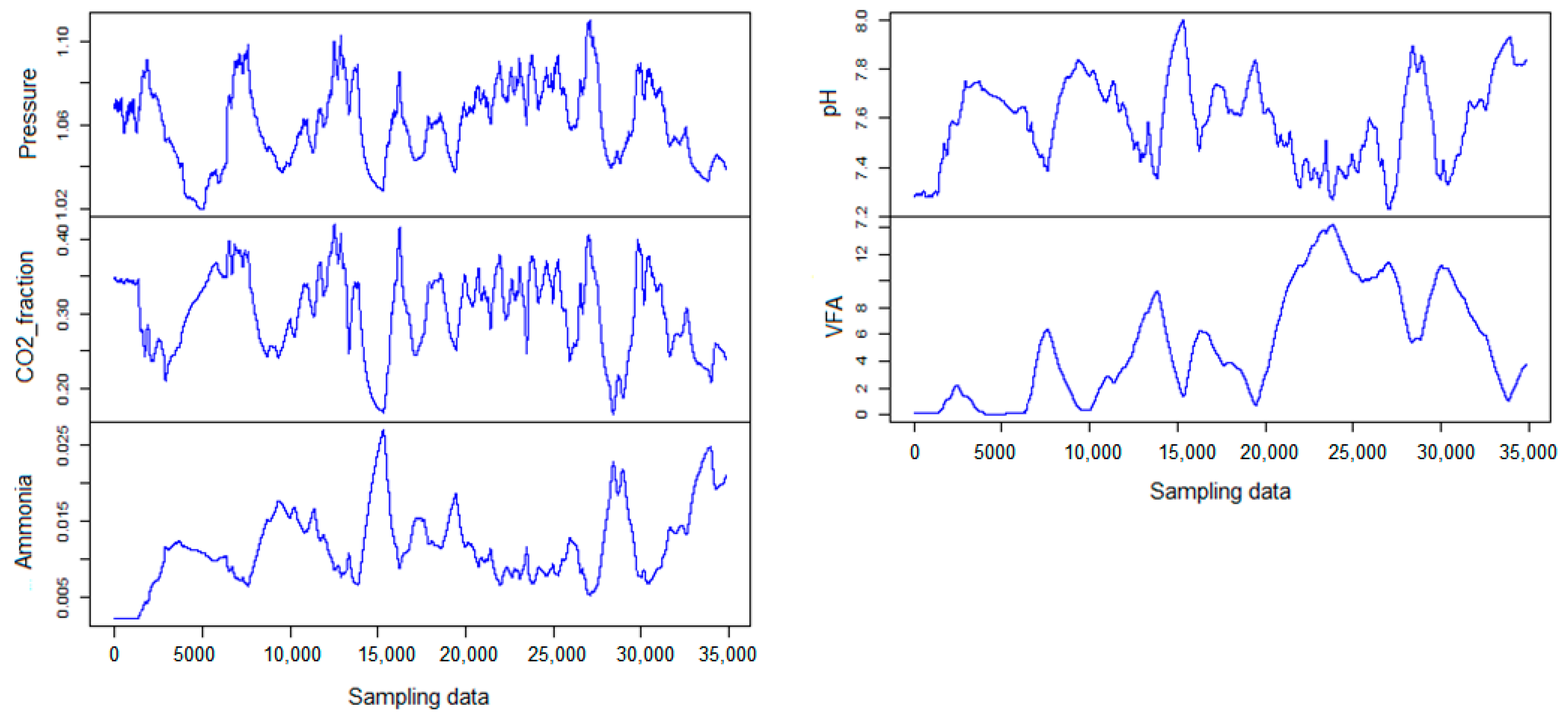
In Figure 4, pH, Ammonia concentration and pressure have the most influence on VFA. To determine the best subset of inputs, we used the SVM method as a non-linear technique. SVM was chosen because it is a fast and accurate method for modelling a non-linear system. Therefore, the most important variables (pH, Ammonia concentration and pressure) were chosen as the core subset and the other variables were added one by one to the model based on their importance values. The validation error is estimated for each subset after the models are trained. Table 5 shows the NRMSE of each subset based on the trained models. It can be seen that the second subset has the best NRMSE; therefore, this subset was selected for further development of VFA soft sensors based on ANN, ELM, SVM and RF. It should be noted that, as the GP model selects influential features inherently, there is no need to perform feature selection before its training. It is interesting that, based on the obtained data set, the flow does not have a significant effect on the VFA compared to the other variables and it is not included in the best subset. Figure 5 shows the trend of four input and output variables over the total experiment period. The input and output trends show that the behavior of the AD process is very complex, which results in absence of direct correlations between parameters.
4.3. Soft Sensor Design
Before the soft sensors were designed, the data set was split into training and validation partitions. The uniformly sampled data from day 245 to 450 were used for training and the rest were used for validation of the final models. All calculations were performed using Amazon Elastic Compute Cloud with 36 cores and 60 GB of random-access memory (RAM) running on the openSUSE operating system (SUSE, Nürnberg, Germany). All modelling procedures were performed in the R environment, except GP, which was developed using the Eureqa Formulize software package [40,41]. This package has been optimized to find simple models, which are expected to have good generalization ability. The tuning parameters of each model were estimated using an extensive grid search. In this method for searching algorithm parameters, a tuning grid must be specified manually. In the grid, each algorithm tuning parameter can be specified as a vector of possible values. These vectors are combined to define all the possible combinations to try. As previously mentioned, different models such as RF, ELM, ANN and SVM have been used to design VFA soft sensors. Each of these models has its own parameters that must be tuned to generate an accurate model. Table 6 shows the final tuning parameters obtained with the grid search. No major parameters need to be tuned for the GP model implemented in the Eureqa Formulize software package.
The NRMSE and R2 are estimated based on the training and validation sets for each model. The results obtained using different techniques are shown in Table 7.
The lowest validation error was achieved by the model developed with the GP algorithm; thus, it should be considered as the final, ready-to-use model. The ANN, ELM and SVM algorithms gave a slightly higher error, but they were still better than the RF model. It can be seen that the RF predictions failed with a NRMSE of 34%. The high error of RF is because it is a rule-based method, in which the data is categorized into different classes. Therefore, if applied to temporal data, weak results will be obtained due to the high number of classes. Although ANN, ELM and SVM are potential non-linear function approximation methods with a broad application, they are still “black box” models whose structure and parameters do not provide any insight into the phenomena underlying the process being modelled. In contrast, the GP model is transparent and can generate explicit equations that are very convenient for direct online implementation in the existing process information and control systems. The GP optimal soft sensor model generated by the Eureqa package is given as a coefficient in Table 8.
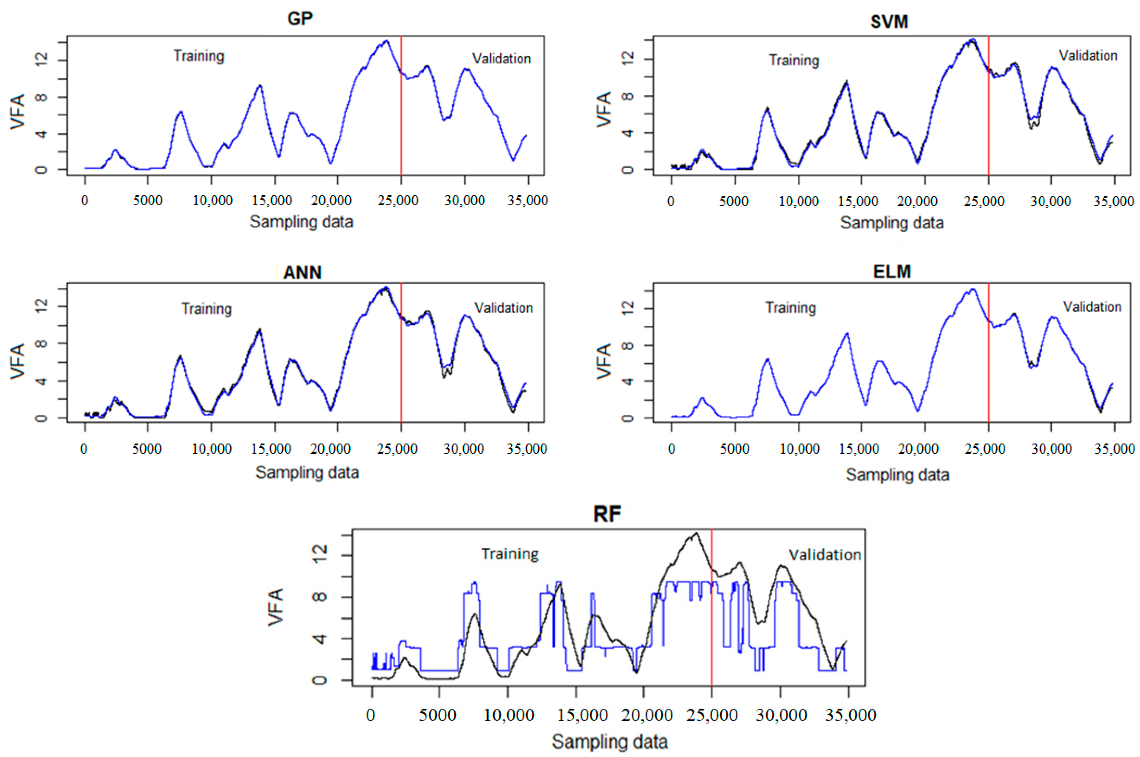
The GP was trained based on the full input vector; however, Table 8 shows that the final model contains four variables. This is in accordance with the result obtained by the fscaret method. In addition, to check the prediction ability of each model, the final models were tested using the whole data set without sampling. Figure 6 shows the prediction result of each model. It can be seen that the performance of all models is satisfactory except for the RF model.
4.4. Evaluation of the Robustness of Soft Sensors
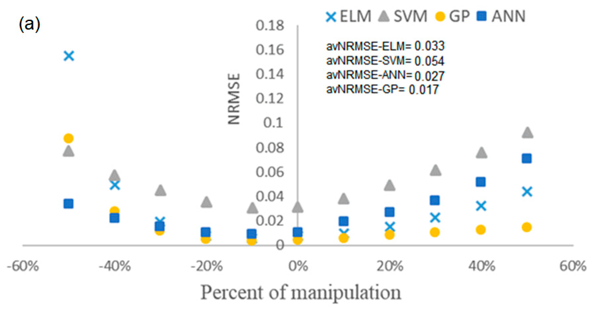
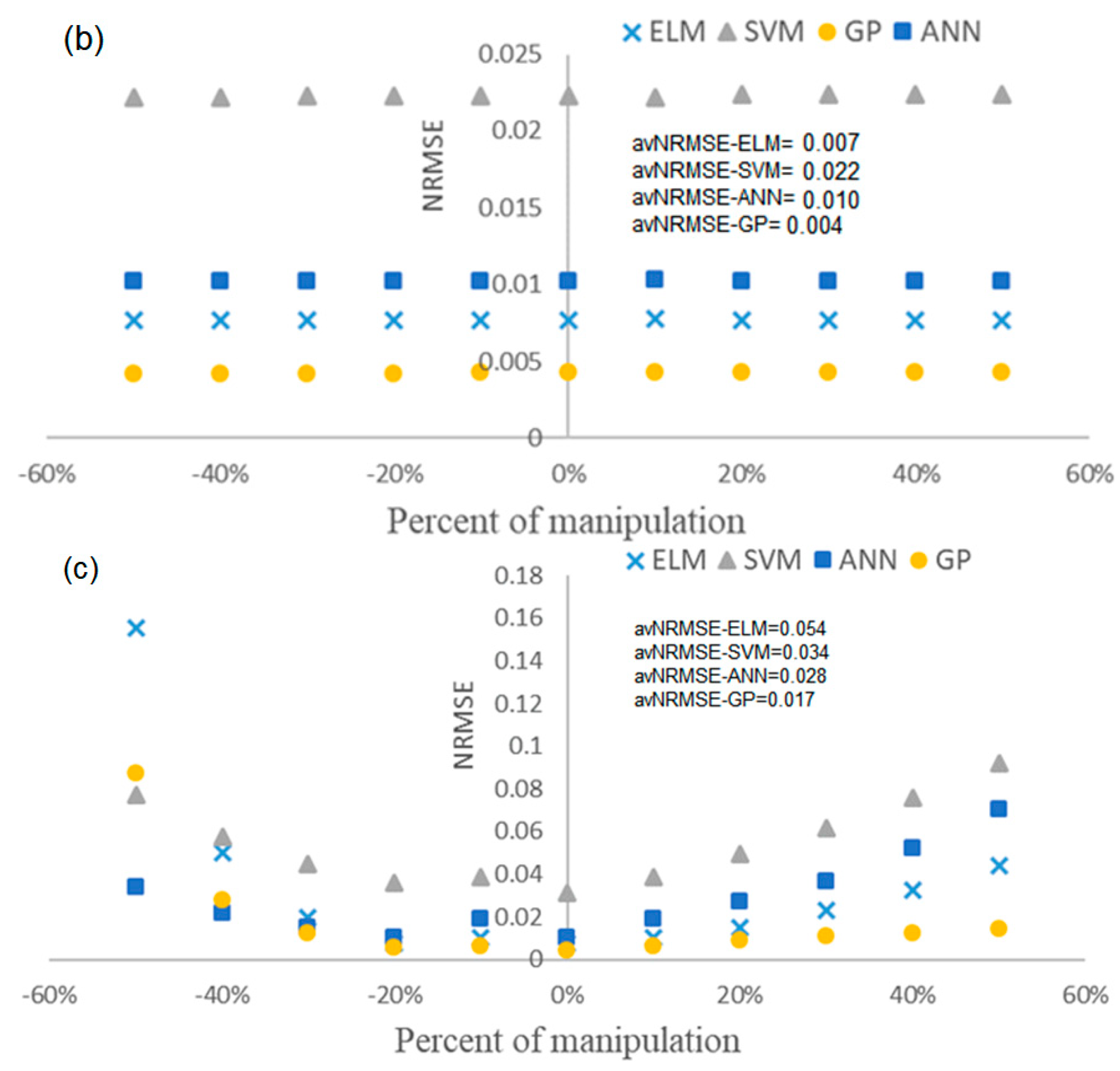
The prediction accuracy of soft sensors tends to drop after a period of their online operation due to changing process states. This change in soft sensor accuracy may cause some issues in the process operation, including increasing the maintenance cost and decreasing the quality of final products. Therefore, it is very beneficial to examine how this accuracy degradation affects the final prediction. To do this, we selected three important biochemical parameters of anaerobic digestion: the hydrolysis rate of carbohydrates (khyd,ch), the maximum uptake rate of acetate (km,ac), and the ammonia inhibition constant (kI,NH3). We then varied them by ±50% around their default values. The default values of khyd,ch, km,ac and kI,NH3 were 10 d−1, 8 d−1 and 0.0018 kmol·m−3 respectively. To evaluate the robustness of each model, new data sets were generated by the BSM2 simulation with modified biochemical parameters. Then, each trained model was tested based on the newly obtained data set. Figure 7 shows the results of the robustness evaluation for each model. As the RF soft sensor failed, it is not considered for the robustness evaluation.
From the variation of km,ac, it can be concluded that GP is the most robust approach, although NRMSE increases at −50%. For khyd,ch, the NRMSE is quite constant which shows that all techniques are insensitive to variations of this parameter; nonetheless, GP still has a lower error compared to the other model. For kI,NH3, again GP is more robust as the error does not change significantly. The least robust model is SVM, which has the highest error compared to the other models. To make comparison easier the average NRMSE for variation of each parameter is also shown in Figure 7.
Comparing avNRMSE for all the soft sensors shows that the GP has lower prediction error during changes in AD state parameters. Overall, the performance of other soft sensor models is also acceptable due to low avNRMSE.
5. Conclusions
In the present paper, different data-driven soft sensors are proposed for predicting the effluent VFA of the AD process. The performance of these soft sensors has been successfully demonstrated with a case study based on synthetic data obtained from BSM2. Analyzing the simulated data with the default BSM2 influent file, the LR models showed that the relationship between input and output data is highly linear. The BSM2 model was modified to introduce non-linearity in the simulated data. Moreover, by applying this modification the behavior of the AD was similar to the anaerobic co-digestion process. The best subset of input variables including pH, ammonia concentration, pressure and CO2 mole fraction was obtained by using the fscaret method along with SVM. After training the models, we obtained the prediction and generalization performances of each model based on a specific validation data set. The results show that all models except RF predict the effluent VFA precisely; however, GP performed slightly better than the other models. The RF model totally failed to predict VFA. This suggests that tree based models are not a very appropriate choice for developing models with an extrapolation capability similar to soft sensors. Assessing the robustness of soft sensors shows that the GP model is more robust and less sensitive to the state changes of the AD process. Last but not least, the other benefit of adopting the GP soft sensor, apart from accuracy and robustness, is its transparency, which makes it easy to integrate into process control systems without any further modifications.
Author Contributions
Conceptualization, P.K. and J.-P.S.; Data curation, P.K. and C.B.; Formal analysis, P.K., J.G. and J.-P.S.; Funding acquisition, J.F.; Investigation, P.K.; Methodology, P.K., J.G. and J.-P.S.; Project administration, J.G. and J.F.; Software, P.K.; Supervision, J.G. and J.F.; Validation, P.K. and J.-P.S.; Visualization, P.K.; Writing–original draft, P.K.; Writing–review & editing, J.F., J.G. and C.B. All authors have read and agreed to the published version of the manuscript.
Funding
This project received support from the Ministerio de Economia, Industria y Competitividad, the Ministerio de Ciencia, Innovación y Universidades, the Agencia Estatal de Investigación (AEI) and the European Regional Development Fund (ERDF), (CTM2015-67970-P, RTI2018-096467-B-I00). This article has been possible due to the support of the Universitat Rovira i Virgili (URV), (2017PFR-URV-B2-33, 2019OPEN) and Fundació Bancària “la Caixa” (2017ARES-06). The authors’ research group is recognized by the Comissionat per a Universitats i Recerca, DIUE de la Generalitat de Catalunya (2017 SGR 396).
Acknowledgments
The authors are very grateful to Ulf Jeppsson from the Lund University, Sweden, for his kindness in providing the BSM2 Matlab code.
Conflicts of Interest
The authors declare no conflict of interest.
References
- Abu Qdais, H.; Bani Hani, K.; Shatnawi, N. Modeling and optimization of biogas production from a waste digester using artificial neural network and genetic algorithm. Resour. Conserv. Recycl. 2010, 54, 359–363. [Google Scholar] [CrossRef]
- Yordanova, S.; Noikova, N.; Petrova, R.; Tzvetkov, P. Neuro-Fuzzy Modelling on Experimental Data in Anaerobic Digestion of Organic Waste in Waters. In Proceedings of the 2005 IEEE Intelligent Data Acquisition and Advanced Computing Systems: Technology and Applications, Sofia, Bulgaria, 5–7 September 2005; IEEE: Piscataway, NJ, USA, 2005; pp. 84–88. [Google Scholar]
- Franke-Whittle, I.H.; Walter, A.; Ebner, C.; Insam, H. Investigation into the effect of high concentrations of volatile fatty acids in anaerobic digestion on methanogenic communities. Waste Manag. 2014, 34, 2080–2089. [Google Scholar] [CrossRef] [PubMed] [Green Version]
- Haimi, H.; Mulas, M.; Corona, F.; Vahala, R. Data-derived soft-sensors for biological wastewater treatment plants: An overview. Environ. Model. Softw. 2013, 47, 88–107. [Google Scholar] [CrossRef]
- Dürrenmatt, D.J.; Gujer, W. Data-driven modeling approaches to support wastewater treatment plant operation. Environ. Model. Softw. 2012, 30, 47–56. [Google Scholar] [CrossRef]
- Corona, F.; Mulas, M.; Haimi, H.; Sundell, L.; Heinonen, M.; Vahala, R. Monitoring nitrate concentrations in the denitrifying post-filtration unit of a municipal wastewater treatment plant. J. Process Control 2013, 23, 158–170. [Google Scholar] [CrossRef]
- Jimenez, J.; Latrille, E.; Harmand, J.; Robles, A.; Ferrer, J.; Gaida, D.; Wolf, C.; Mairet, F.; Bernard, O.; Alcaraz-Gonzalez, V.; et al. Instrumentation and control of anaerobic digestion processes: A review and some research challenges. Rev. Environ. Sci. Bio/Technol. 2015, 14, 615–648. [Google Scholar] [CrossRef]
- James, S.C.; Legge, R.L.; Budman, H. On-line estimation in bioreactors: A review. Rev. Chem. Eng. 2000, 16, 311–340. [Google Scholar] [CrossRef]
- Gernaey, K.V.; Van Loosdrecht, M.C.M.; Henze, M.; Lind, M.; Jørgensen, S.B. Activated sludge wastewater treatment plant modelling and simulation: State of the art. Environ. Model. Softw. 2004, 19, 763–783. [Google Scholar] [CrossRef]
- Newhart, K.B.; Holloway, R.W.; Hering, A.S.; Cath, T.Y. Data-driven performance analyses of wastewater treatment plants: A review. Water Res. 2019, 157, 498–513. [Google Scholar] [CrossRef]
- Corominas, L.; Garrido-Baserba, M.; Villez, K.; Olsson, G.; Cort Es, U.; Poch, M. Transforming data into knowledge for improved wastewater treatment operation: A critical review of techniques. Environ. Model. Softw. 2018, 106, 89–103. [Google Scholar] [CrossRef]
- Tay, J.-H.; Zhang, X. A fast predicting neural fuzzy model for high-rate anaerobic wastewater treatment systems. Water Res. 2000, 34, 2849–2860. [Google Scholar] [CrossRef]
- Mullai, P.; Arulselvi, S.; Ngo, H.-H.; Sabarathinam, P.L. Experiments and ANFIS modelling for the biodegradation of penicillin-G wastewater using anaerobic hybrid reactor. Bioresour. Technol. 2011, 102, 5492–5497. [Google Scholar] [CrossRef] [PubMed]
- Güçlü, D.; Yılmaz, N.; Ozkan-Yucel, U.G. Application of neural network prediction model to full-scale anaerobic sludge digestion. J. Chem. Technol. Biotechnol. 2011, 86, 691–698. [Google Scholar] [CrossRef]
- Rangasamy, P.; Pvr, I.; Ganesan, S. Anaerobic tapered fluidized bed reactor for starch wastewater treatment and modeling using multilayer perceptron neural network. J. Environ. Sci. 2007, 19, 1416–1423. [Google Scholar] [CrossRef]
- Huang, M.; Han, W.; Wan, J.; Ma, Y.; Chen, X. Multi-objective optimisation for design and operation of anaerobic digestion using GA-ANN and NSGA-II. J. Chem. Technol. Biotechnol. 2016, 91, 226–233. [Google Scholar] [CrossRef]
- Beltramo, T.; Klocke, M.; Hitzmann, B. Prediction of the biogas production using GA and ACO input features selection method for ANN model. Inf. Process. Agric. 2019, 6, 349–356. [Google Scholar] [CrossRef]
- Jeppsson, U.; Rosen, C.; Alex, J.; Copp, J.; Gernaey, K.V.; Pons, M.-N.; Vanrolleghem, P.A. Towards a benchmark simulation model for plant-wide control strategy performance evaluation of WWTPs. Water Sci. Technol. 2006, 53, 287–295. [Google Scholar] [CrossRef]
- Nopens, I.; Benedetti, L.; Jeppsson, U.; Pons, M.-N.; Alex, J.; Copp, J.B.; Gernaey, K.V.; Rosen, C.; Steyer, J.-P.; Vanrolleghem, P.A. Benchmark Simulation Model No 2: Finalisation of plant layout and default control strategy. Water Sci. Technol. 2010, 62, 1967–1974. [Google Scholar] [CrossRef]
- Hota, H.S.; Handa, R.; Shrivas, A.K. Time series data prediction using sliding window based Rbf neural network. Int. J. Comput. Intell. Res. 2017, 13, 1145–1156. [Google Scholar]
- Gil, J.D.; Ruiz-Aguirre, A.; Roca, L.; Zaragoza, G.; Berenguel, M. Prediction models to analyse the performance of a commercial-scale membrane distillation unit for desalting brines from RO plants. Desalination 2018, 445, 15–28. [Google Scholar] [CrossRef] [Green Version]
- Eskandarian, S.; Bahrami, P.; Kazemi, P. A comprehensive data mining approach to estimate the rate of penetration: Application of neural network, rule based models and feature ranking. J. Pet. Sci. Eng. 2017, 156, 605–615. [Google Scholar] [CrossRef]
- Stanley, K.O.; Miikkulainen, R. Evolving Neural Networks through Augmenting Topologies. Evol. Comput. 2002, 10, 99–127. [Google Scholar] [CrossRef] [PubMed]
- R Core Team. R: A Language and Environment for Statistical Computing; R Foundation for Statistical Computing: Vienna, Austria, 2018. [Google Scholar]
- Candel, A.; Ledell, E.; Bartz, A. Deep Learning with H2O. Available online: https://h2o-release.s3.amazonaws.com/h2o/rel-wright/9/docs-website/h2o-docs/booklets/DeepLearningBooklet.pdf (accessed on 11 November 2019).
- Huang, G.B.; Zhu, Q.Y.; Siew, C.K. Extreme learning machine: A new learning scheme of feedforward neural networks. In Proceedings of the 2004 IEEE International Joint Conference on Neural Networks (IEEE Cat. No.04CH37541), Budapest, Hungary, 25–29 July 2004; IEEE: Piscataway, NJ, USA, 2004; Volume 2, pp. 985–990. [Google Scholar]
- Abdullah, S.S.; Malek, M.A.; Abdullah, N.S.; Kisi, O.; Yap, K.S. Extreme Learning Machines: A new approach for prediction of reference evapotranspiration. J. Hydrol. 2015, 527, 184–195. [Google Scholar] [CrossRef]
- Zhang, C.; Liu, Q.; Wu, Q.; Zheng, Y.; Zhou, J.; Tu, Z.; Chan, S.H. Modelling of solid oxide electrolyser cell using extreme learning machine. Electrochim. Acta 2017, 251, 137–144. [Google Scholar] [CrossRef]
- Breiman, L. Random Forests. Mach. Learn. 2001, 45, 5–32. [Google Scholar] [CrossRef] [Green Version]
- Cortes, C.; Vapnik, V. Support-Vector Networks. Mach. Learn. 1995, 20, 273–297. [Google Scholar] [CrossRef]
- Smola, A.J.; Schölkopf, B. A tutorial on support vector regression. Stat. Comput. 2004, 14, 199–222. [Google Scholar] [CrossRef] [Green Version]
- Najafzadeh, M.; Etemad-Shahidi, A.; Lim, S.Y. Scour prediction in long contractions using ANFIS and SVM. Ocean Eng. 2016, 111, 128–135. [Google Scholar] [CrossRef]
- Liu, L.; Lei, Y. An accurate ecological footprint analysis and prediction for Beijing based on SVM model. Ecol. Inform. 2018, 44, 33–42. [Google Scholar] [CrossRef]
- Koza, J. Genetic programming as a means for programming computers by natural selection. Stat. Comput. 1994, 4, 87–112. [Google Scholar] [CrossRef]
- Bahrami, P.; Kazemi, P.; Mahdavi, S.; Ghobadi, H. A novel approach for modeling and optimization of surfactant/polymer flooding based on Genetic Programming evolutionary algorithm. Fuel 2016, 179, 289–298. [Google Scholar] [CrossRef]
- Sonolikar, R.R.; Patil, M.P.; Mankar, R.B.; Tambe, S.S.; Kulkarni, B.D. Genetic Programming based Drag Model with Improved Prediction Accuracy for Fluidization Systems. Int. J. Chem. React. Eng. 2017, 15. [Google Scholar] [CrossRef]
- James, G.; Witten, D.; Hastie, T.; Tibshirani, R. An Introduction to Statistical Learning; Springer Texts in Statistics; Springer: New York, NY, USA, 2013; Volume 103, ISBN 978-1-4614-7137-0. [Google Scholar]
- Szlęk, J.; Mendyk, A. Fscaret: Automated Feature Selection from ‘Caret’ [Software]. Available online: https://cran.r-project.org/web/packages/fscaret/index.html (accessed on 10 March 2018).
- Szlęk, J.; Pacławski, A.; Lau, R.; Jachowicz, R.; Kazemi, P.; Mendyk, A. Empirical search for factors affecting mean particle size of PLGA microspheres containing macromolecular drugs. Comput. Methods Programs Biomed. 2016, 134, 137–147. [Google Scholar] [CrossRef] [PubMed]
- Schmidt, M.; Lipson, H. Distilling Free-Form Natural Laws from Experimental Data. Science 2009, 324, 81–85. [Google Scholar] [CrossRef] [PubMed]
- Schmidt, M.; Hod, L.; Schmidt, M.; Lipson, H. Eureqa (Version 0.98 Beta) [Software]. 2013. Available online: http://www.eureqa.com/ (accessed on 4 May 2018).
Figure 1.
Simple scheme of a neuron.

Figure 2.
Scheme of the extreme learning machine (ELM) model.

Figure 3.
Computation flowchart of genetic programming (GP).

Figure 4.
Importance of variables on a scale from 0 to 100 obtained with the fscaret method.

Figure 5.
Trend of input and output variables used for developing soft sensors.

Figure 6.
Prediction results of different soft sensors; black is the actual values and blue is the predicted volatile fatty acid (VFA) values. GP: genetic programming; SVM: support vector machine; ANN: artificial neural network; ELM: extreme learning machine; RF: random forest.
Figure 6.
Prediction results of different soft sensors; black is the actual values and blue is the predicted volatile fatty acid (VFA) values. GP: genetic programming; SVM: support vector machine; ANN: artificial neural network; ELM: extreme learning machine; RF: random forest.

Figure 7.
Results of the robustness evaluation for each model: (a) for km,ac; (b) for khyd,ch; (c) for kI,NH3. NRMSE: normalized root-mean-squared error; avNRMSE: average normalized root-mean-squared error.
Figure 7.
Results of the robustness evaluation for each model: (a) for km,ac; (b) for khyd,ch; (c) for kI,NH3. NRMSE: normalized root-mean-squared error; avNRMSE: average normalized root-mean-squared error.


Table 1.
Obtained variables from Benchmark Simulation Model No. 2 (BSM2).
| Parameters | Unit | Parameters | Unit |
|---|---|---|---|
| Effluent COD | g m−3 | CH4 mol_fraction | - |
| Effluent alkalinity | Mol m−3 | CO2 mol_fraction | - |
| Influent TSS | g m−3 | H2 mol_fraction | - |
| Effluent TSS | g m−3 | Pressure | bar |
| Effluent pH | - | Effluent ammonia | g m−3 |
| Effluent BOD | g m−3 | Influent Flow | m3 d−1 |
| Gas flow | m3 d−1 |
COD: chemical oxygen demand; TSS: total soluble solid; BOD: biological oxygen demand.
Table 2.
Performance of the linear regression (LR) models based on the default influent file and different input vectors.
Table 2.
Performance of the linear regression (LR) models based on the default influent file and different input vectors.
| All_Inputs | All_Input_Except _TSS | All_Input_Except _Ammonia | All_Input_Except _TSS & Ammonia | |
|---|---|---|---|---|
| Training_NRMSE | 0.028 | 0.029 | 0.028 | 0.029 |
| Test_NRMSE | 0.039 | 0.039 | 0.038 | 0.038 |
| Training_R2 | 0.981 | 0.978 | 0.979 | 0.976 |
| Test_R2 | 0.967 | 0.966 | 0.967 | 0.968 |
NRMSE: normalized root-mean-squared error; R2: coefficient of determination.
Table 3.
Summary of default and the modified values of inorganic nitrogen (Sin), composite (Xc) and carbohydrate (Xch).
Table 3.
Summary of default and the modified values of inorganic nitrogen (Sin), composite (Xc) and carbohydrate (Xch).
| Default Values | Modified Values | |||||||
|---|---|---|---|---|---|---|---|---|
| Sin (kmol m−3) | Xc (kg m−3) | Xch (kg m−3) | Flow (m3 d−1) | Sin (kmol m−3) | Xc (kg m−3) | Xch (kg m−3) | Flow (m3 d−1) | |
| Min. | 0.0006 | 0 | 0.000 | 56.55 | 0.0006 | 0.00 | 0.000 | 1.993 |
| 1st Qu. | 0.0015 | 0 | 2.941 | 137.07 | 0.0019 | 0.00 | 3.293 | 82.257 |
| Median | 0.0019 | 0 | 3.952 | 175.81 | 0.1156 | 22.54 | 4.897 | 138.704 |
| Mean | 0.0020 | 0 | 3.830 | 183.57 | 0.0957 | 16.41 | 7.256 | 140.602 |
| 3rd Qu. | 0.0022 | 0 | 4.833 | 217.90 | 0.1584 | 28.71 | 9.684 | 193.301 |
| Max. | 0.0325 | 0 | 8.607 | 479.96 | 0.2718 | 39.52 | 40.464 | 477.957 |
Table 4.
Performance of the LR models based on the modified anaerobic digestion (AD) variables and different input vectors.
Table 4.
Performance of the LR models based on the modified anaerobic digestion (AD) variables and different input vectors.
| All_Inputs | All_Input_Except _TSS | All_Input_Except _Ammonia | All_Input_Except _TSS & Ammonia | |
|---|---|---|---|---|
| Training_NRMSE | 0.103 | 0.133 | 0.143 | 0.189 |
| Test_NRMSE | 0.197 | 0.213 | 0.122 | 0.304 |
| Training_R2 | 0.865 | 0.794 | 0.748 | 0.586 |
| Test_R2 | 0.654 | 0.511 | 0.841 | 0.663 |
Table 5.
Result of different subsets trained by support vector machine (SVM).
| Inputs | R2 | NRMSE |
|---|---|---|
| pH + Ammonia_conc + pressure | 0.813 | 0.182 |
| pH + Ammonia_conc + pressure + CO2_mol fraction | 0.990 | 0.033 |
| pH + Ammonia_conc + pressure + CO2_mol_fraction + TSS_out | 0.972 | 0.058 |
| pH + Ammonia_conc + pressure + CO2_mol_fraction + TSS_out+Flow | 0.977 | 0.044 |
| pH + Ammonia_conc + pressure + CO2_mol_fraction + TSS_out + Flow + H2_mol_fraction | 0.971 | 0.049 |
Table 6.
Final tuning parameters of soft sensors obtained with the grid search.
| Algorithm | Tuning Parameters | ||||
|---|---|---|---|---|---|
| ANN | Neuron Size | Transfer Function | Number of Hidden Layers | L1 | L2 |
| 108 | Tanh | 1 | 1 × 10⁻⁵ | 1 × 10⁻⁵ | |
| RF | mtry | Number of trees | Maximum nodes | ||
| 4 | 1600 | 20 | |||
| ELM | Neuron size | Transfer function | |||
| 126 | Sigmoid | ||||
| SVM | Sigma | C | |||
| 0.2 | 500 | ||||
ANN: artificial neural network; RF: random forest; ELM: extreme learning machine; SVM: support vector machine.
Table 7.
Results of soft sensors for the training and validation sets.
| Algorithm | NRMSE Training | R2 Training | NRMSE Validation | R2 Validation |
|---|---|---|---|---|
| ANN | 0.0089 | 0.9992 | 0.0192 | 0.9969 |
| RF | 0.1432 | 0.7533 | 0.3419 | 0.5784 |
| ELM | 0.0003 | 0.9999 | 0.0169 | 0.9977 |
| SVM | 0.0165 | 0.9966 | 0.0390 | 0.9941 |
| GP | 0.0025 | 0.9999 | 0.0037 | 0.9998 |
GP: genetic programming.
Table 8.
Coefficient table for the equation obtained by GP.
| Term * | Coef | Term * | Coef |
|---|---|---|---|
| constant | |||
* , , , and correspond to the ammonia concentration, pH, CO2 fraction and pressure, respectively.
© 2020 by the authors. Licensee MDPI, Basel, Switzerland. This article is an open access article distributed under the terms and conditions of the Creative Commons Attribution (CC BY) license (http://creativecommons.org/licenses/by/4.0/).
Share and Cite
MDPI and ACS Style
Kazemi, P.; Steyer, J.-P.; Bengoa, C.; Font, J.; Giralt, J. Robust Data-Driven Soft Sensors for Online Monitoring of Volatile Fatty Acids in Anaerobic Digestion Processes. Processes 2020, 8, 67. https://doi.org/10.3390/pr8010067
AMA Style
Kazemi P, Steyer J-P, Bengoa C, Font J, Giralt J. Robust Data-Driven Soft Sensors for Online Monitoring of Volatile Fatty Acids in Anaerobic Digestion Processes. Processes. 2020; 8(1):67. https://doi.org/10.3390/pr8010067
Chicago/Turabian StyleKazemi, Pezhman, Jean-Philippe Steyer, Christophe Bengoa, Josep Font, and Jaume Giralt. 2020. "Robust Data-Driven Soft Sensors for Online Monitoring of Volatile Fatty Acids in Anaerobic Digestion Processes" Processes 8, no. 1: 67. https://doi.org/10.3390/pr8010067
Note that from the first issue of 2016, this journal uses article numbers instead of page numbers. See further details here.