
Predicting the Ultimate Axial Capacity of Uniaxially Loaded CFST Columns Using Multiphysics Artificial Intelligence

 ,
,  , , and
Abstract
:1. Introduction
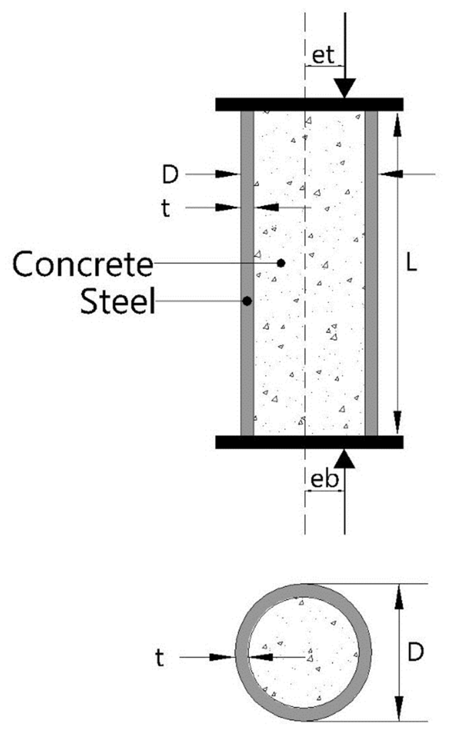
1.1. Concrete Filled Steel Tube Artificial Modelling
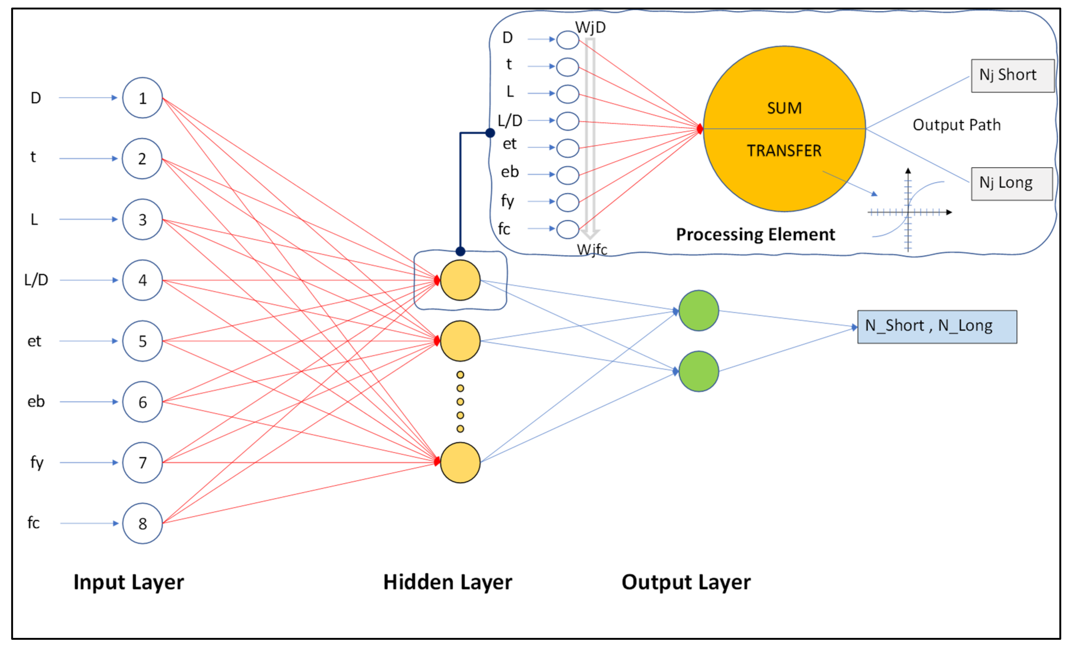
1.2. Detailed Description of Machine Learning Algorithms (ANN, ANFIS, GEP)
- (a)
- data collection,
- (b)
- ANFIS growth,
- (c)
- variables selection,
- (d)
- training and testing,
- (e)
- results
1.2.1. Layer 1
1.2.2. Layer 2
1.2.3. Layer 3
1.2.4. Layer 4
1.2.5. Layer 5
- (a)
- Head consisting of function or terminal symbols
- (b)
- Tail containing only the terminal symbols.
1.3. The Aim of the Research
2. Methods
2.1. Description and Division of Collected Data
2.2. Structure of ANN, ANFIS and GEP Models
2.3. Evaluation of Models through Statistical Measures
3. Results and Discussion
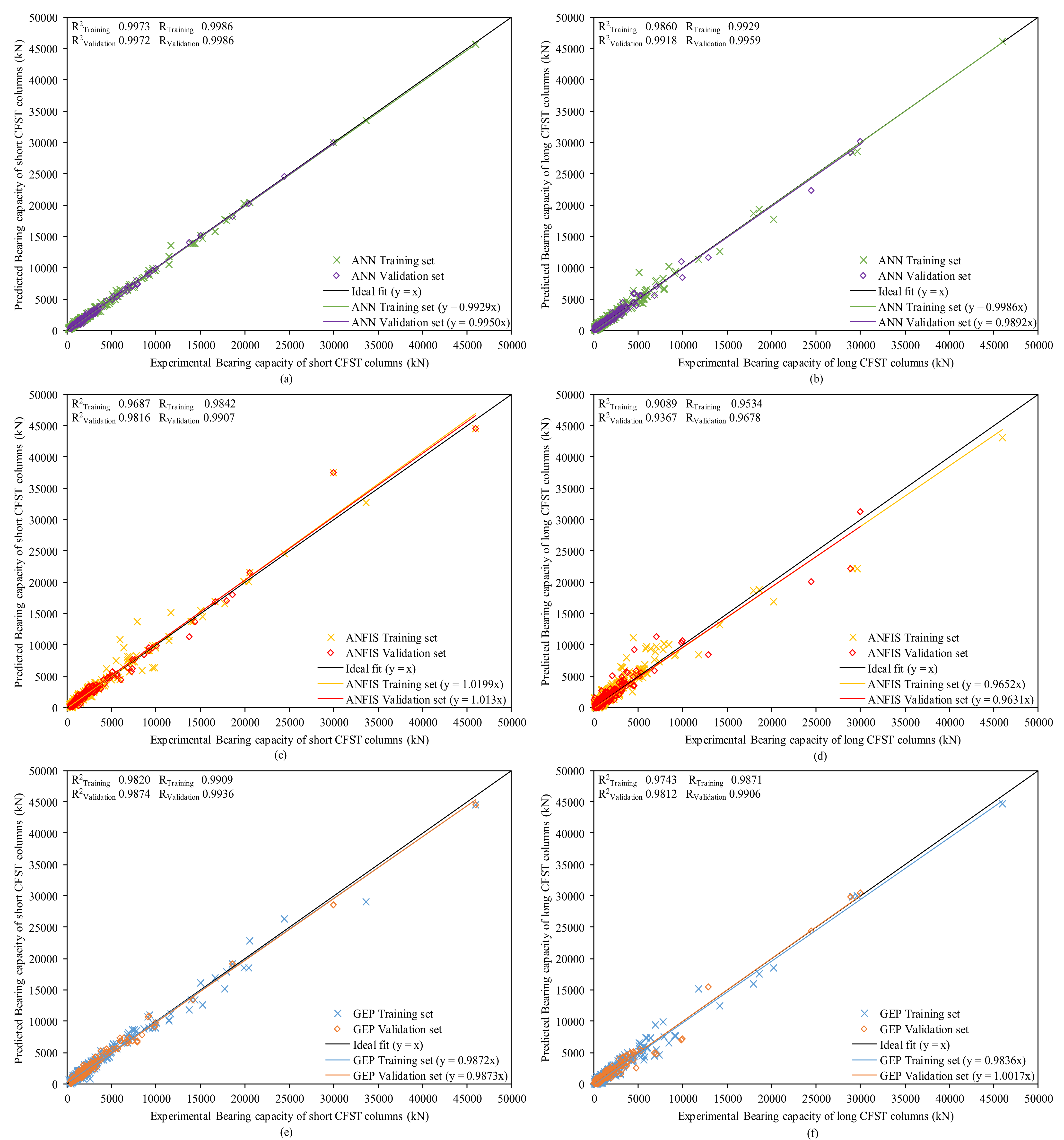
3.1. Regression Analysis of ANN, ANFIS and GEP Model
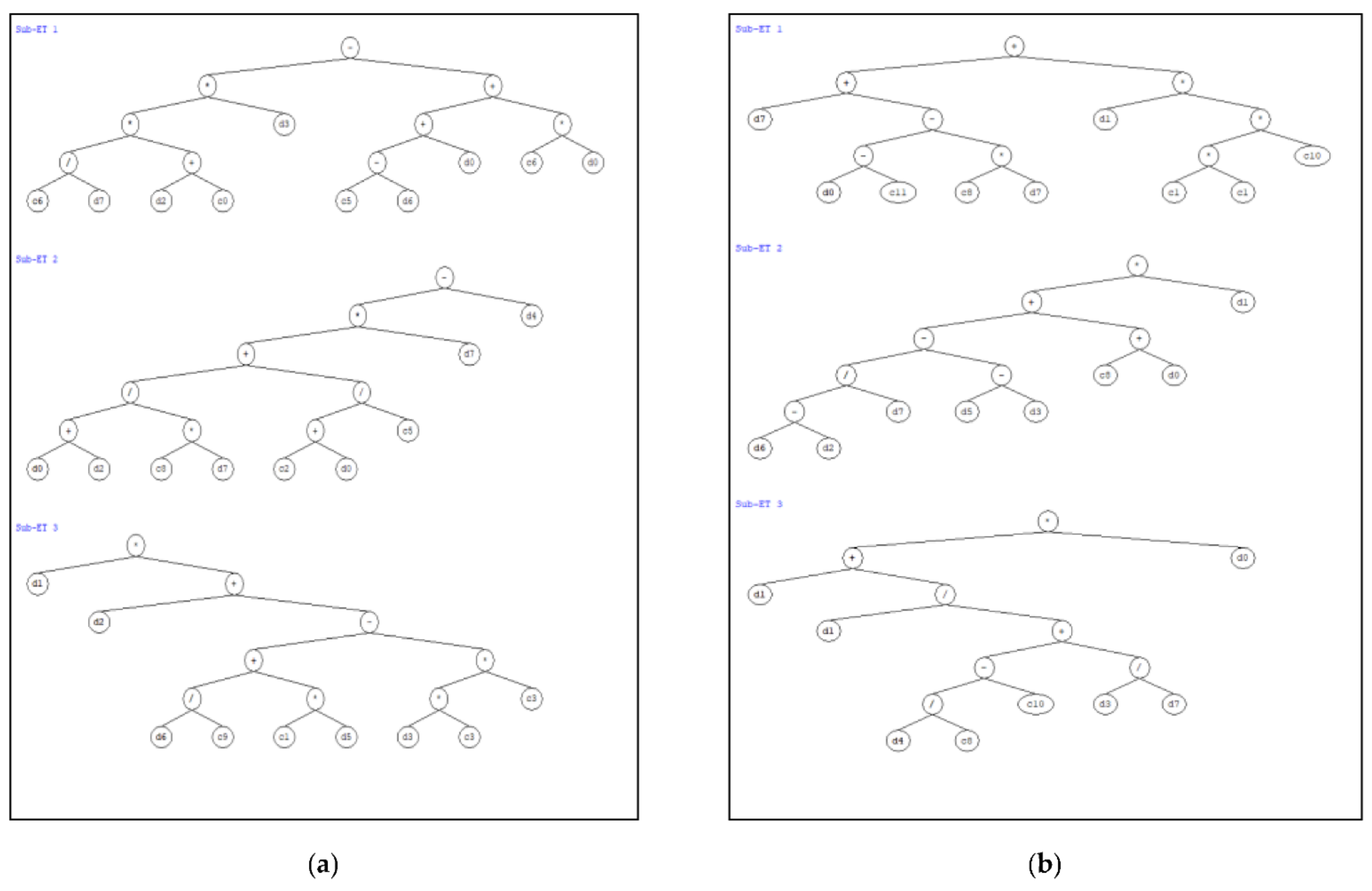
3.2. GEP Based Formulation of Bearing Capacity of CFST Columns
3.3. Performance Evaluation of Proposed Models Using Statistical Indicators
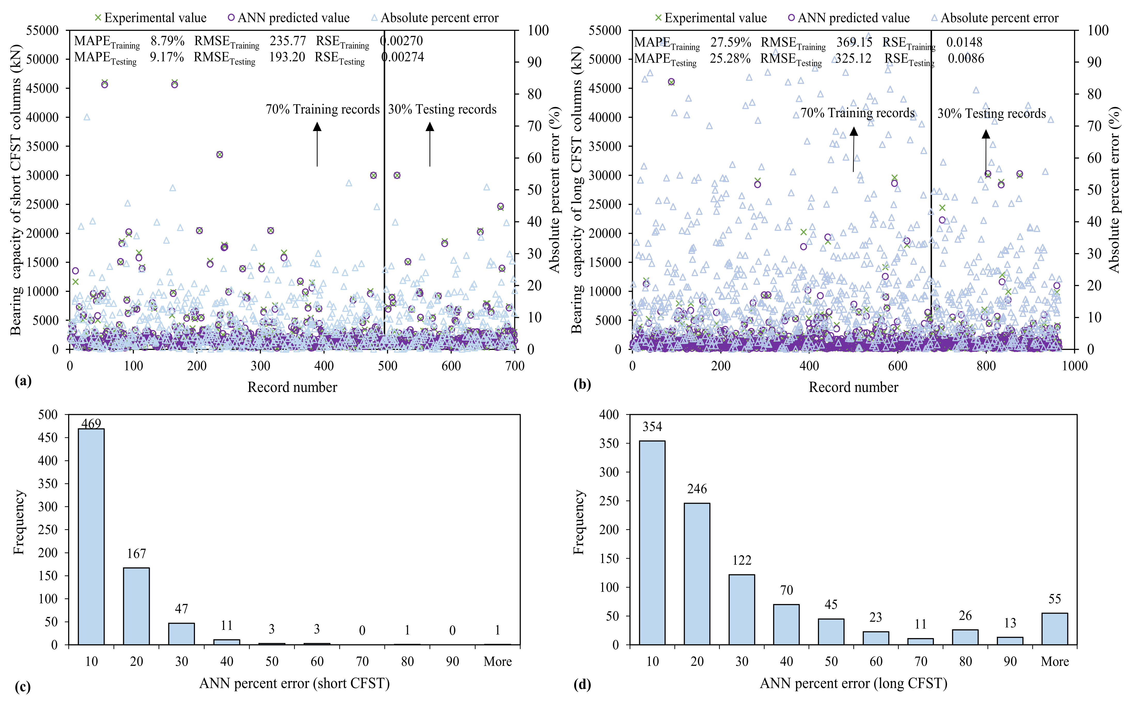
3.3.1. ANN Model
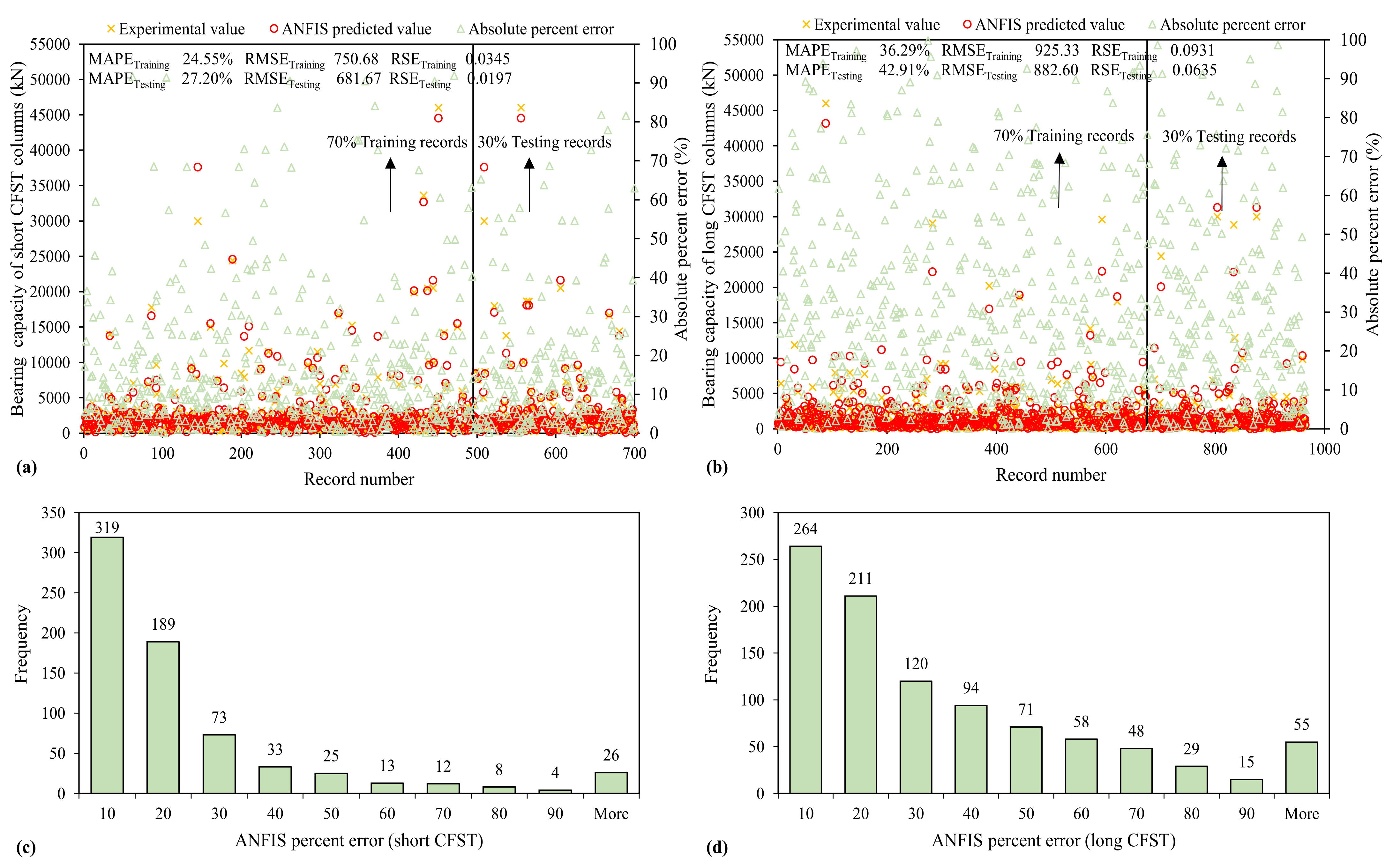
3.3.2. ANFIS
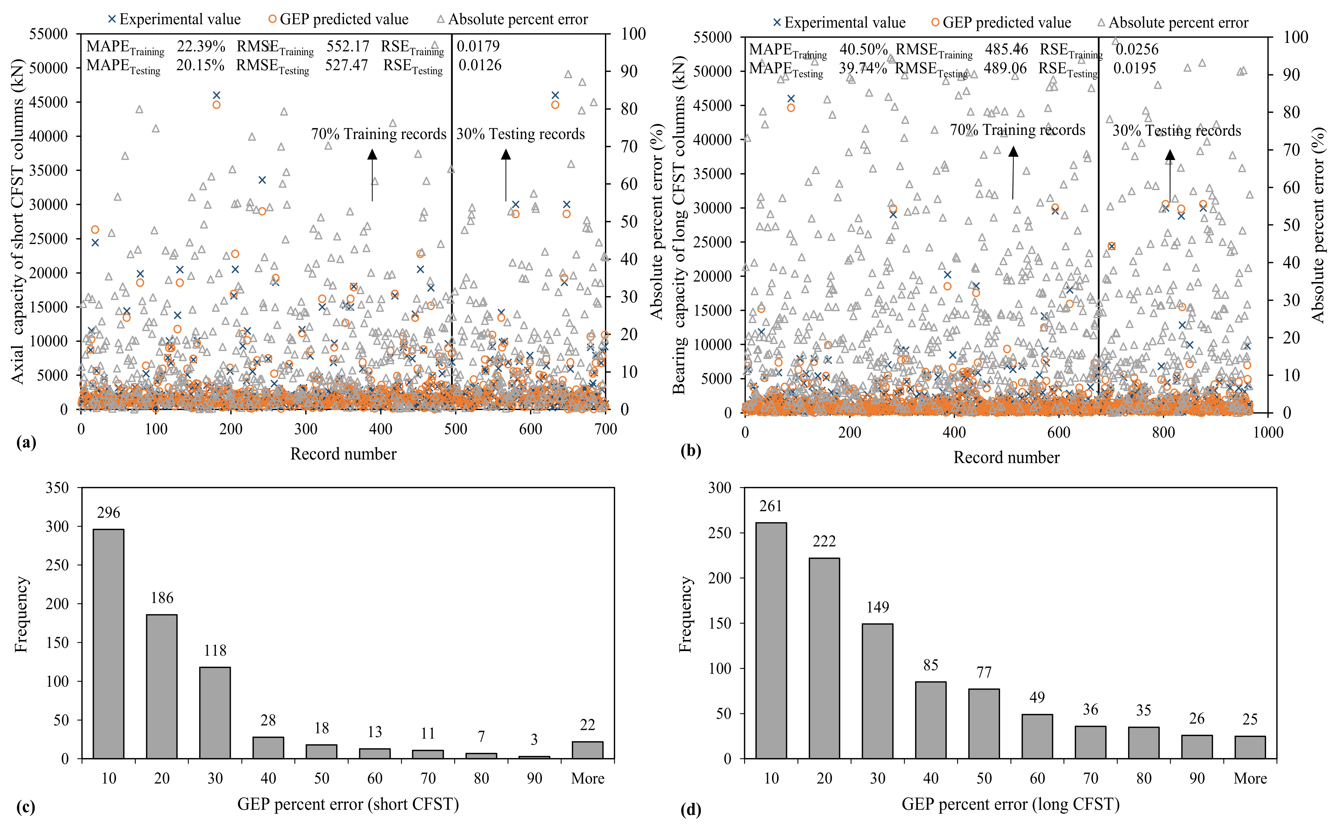
3.3.3. GEP Model
3.4. Comparison of Models Using External Testing Criteria
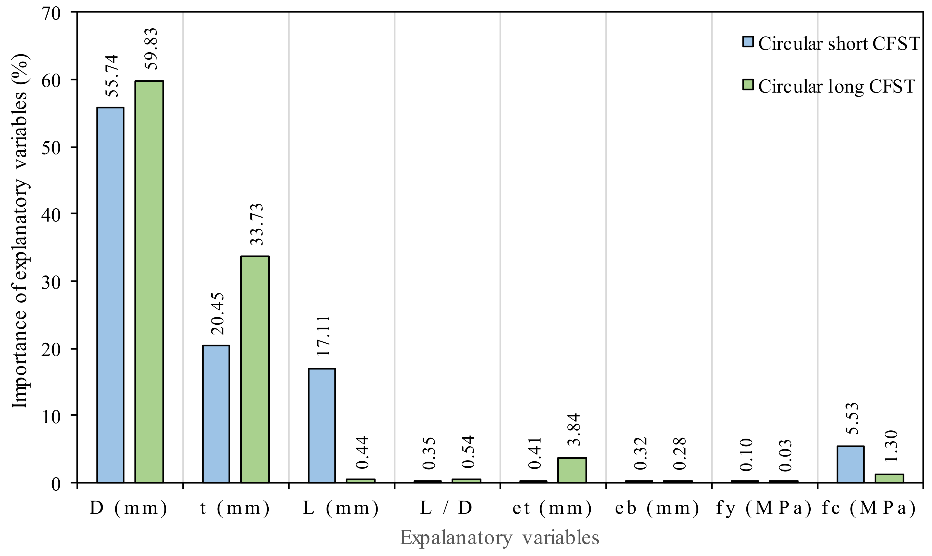
3.5. Sensitivity and Parametric Study of GEP Models
4. Conclusions
- The GEP model can efficiently predict Nst and Nlg with high accuracy and best performance. Moreover, the bearing capacity prediction model from GEP is better than the ANFIS and ANN models. The diversity of the GEP technique can be seen from the simplified formulation, with higher accuracy and correlation among the experimental and predicted data with the consideration of linear and non-linear data.
- The statistical indicators used to evaluate the performance of the model were mean absolute error (MAE), root square error (RSE), root means square error (RMSE), correlation coefficient (R), relative root mean square error (RRMSE), performance index (PI) and objective function (OF). The PI of the predicted Nst by GEP, ANN and ANFIS for training are 0.0416, 0.1423, and 0.1016, respectively, and for Nlg these values are 0.1169, 0.2990 and 0.1542, respectively. Corresponding OF values are 0.2300, 0.1200, and 0.090 for Nst, and 0.1000, 0.2700, and 0.1500 for Nlg. The superiority of the GEP method to the other techniques can be seen from the fact that the GEP technique provides suitable connections based on the practical experimental work and does not undertake prior solutions. In reference to MAPE indicator, the ANN provides excellent forecasting results for Nst, while all other models including Nlg-ANN fall in the “acceptable prediction” category.
- Sensitivity analysis was performed and the following input importance with increasing pattern was observed for Nst: D (55.45) > T (20.45) > L (17.109) > fc (5.526) > et (0.41) > L/D (0.34) > eb (0.32) > fy (0.096); whereas, in the case of Nlg, it followed the order: D (59.83) > T (33.73) > et (3.844) > fc (1.302) > L/D (0.541) > L (0.443) > eb (0.282) > fy (0.033). Parametric analysis showed a trend similar to the findings in previous literature. The effect of input parameters on the bearing capacity of circular short (Nst) and long (Nlg) CFST columns was studied. Thus, it can be concluded from this research that artificial intelligence techniques can be effectively employed to solve various complex engineering problems, especially in structural and material engineering. A simple, reliable, and accurate model can be developed which can perform better on unseen data.
- The overall comparison shows that the most reliable and accurate technique for developing prediction models is GEP. The prediction models developed through the GEP technique are simpler than ANN and ANFIS models. It is, therefore, suggested that the developed GEP equations (Equations (22) and (23)) are used in routine design for circular short (Nst) and long (Nlg) CFST columns with eccentric loading using simple geometric and material properties. These models can replace tedious, time consuming and costly experimental work for finding the bearing capacity of CFST columns.
Author Contributions
Funding
Institutional Review Board Statement
Informed Consent Statement
Data Availability Statement
Acknowledgments
Conflicts of Interest
References
- Romero, M.L.; Espinós, A.; Lapuebla-Ferri, A.; Albero, V.; Hospitaler, A. Recent developments and fire design provisions for CFST columns and slim-floor beams. J. Constr. Steel Res. 2020, 172, 106159. [Google Scholar] [CrossRef]
- Suizi, J.; Wanlin, C.; Zibin, L.; Wei, D.; Yingnan, S. Experimental study on a prefabricated lightweight concrete-filled steel tubular framework composite slab structure subjected to reversed cyclic loading. Appl. Sci. 2019, 9, 1264. [Google Scholar] [CrossRef] [Green Version]
- Ayough, P.; Ibrahim, Z.; Sulong, N.R.; Hsiao, P.-C. The effects of cross-sectional shapes on the axial performance of concrete-filled steel tube columns. J. Constr. Steel Res. 2021, 176, 106424. [Google Scholar] [CrossRef]
- Ibañez, C.; Hernández-Figueirido, D.; Piquer, A. Shape effect on axially loaded high strength CFST stub columns. J. Constr. Steel Res. 2018, 147, 247–256. [Google Scholar] [CrossRef]
- Phan, D.H.H.; Patel, V.I.; Al Abadi, H.; Thai, H.-T. Analysis and design of eccentrically compressed ultra-high-strength slender CFST circular columns. Structures 2020, 27, 2481–2499. [Google Scholar] [CrossRef]
- Thai, S.; Thai, H.-T.; Uy, B.; Ngo, T. Concrete-filled steel tubular columns: Test database, design and calibration. J. Constr. Steel Res. 2019, 157, 161–181. [Google Scholar] [CrossRef]
- Chinese, S. Technical Code for Concrete Filled Steel Tubular Structures; GB 50936; Ministry of Housing and Urban Rural Construction of the People’s Republic of China: Beijing, China, 2014.
- AIJ. Recommendations for Design and Construction of Concrete Filled Steel Tubular Structures; AIJ: Tokyo, Japan, 1997. [Google Scholar]
- ANSI/AISC 360-05. Specification for Structural Steel Buildings; American Institute of Steel Construction: Chicago, IL, USA, 2016; p. 586. [Google Scholar]
- Uy, B.; Hicks, S.J.; Kang, W.-H.; Thai, H.-T.; Aslani, F. The New Australia/New Zealand Standard on Composite Steel-Concrete Buildings. In Proceedings of the 8th International Conference on Composite Construction in Steel and Concrete, Jackson, WY, USA, 30 July–2 August 2017. ASNZS2327. [Google Scholar]
- European Committee for Standardization. 1-1; Eurocode 4: Design of Composite Steel and Concrete Structures—Part 1-1: General Rules and Rules for Buildings; Europian Committee for Standardization: Brussels, Belgium, 2004. [Google Scholar]
- Liew, J.R. Design Guide for Concrete Filled Tubular Members with High Strength Materials to Eurocode 4; Research Publishing: Singapore, 2015; ISBN 978-981-09-3267-1. [Google Scholar]
- Khan, M.; Uy, B.; Tao, Z.; Mashiri, F. Behaviour and design of short high-strength steel welded box and concrete-filled tube (CFT) sections. Eng. Struct. 2017, 147, 458–472. [Google Scholar] [CrossRef]
- Mursi, M.; Uy, B. Strength of slender concrete filled high strength steel box columns. J. Constr. Steel Res. 2004, 60, 1825–1848. [Google Scholar] [CrossRef]
- Vatulia, G.; Orel, Y.; Rezunenko, M.; Panchenko, N. Using statistical methods to determine the load-bearing capacity of rectangular CFST columns. MATEC Web Conf. 2018, 234, 04002. [Google Scholar] [CrossRef]
- Le, T.-T. Practical machine learning-based prediction model for axial capacity of square CFST columns. Mech. Adv. Mater. Struct. 2020, 1–16. [Google Scholar] [CrossRef]
- Mai, S.H.; Seghier, M.; Nguyen, P.L.; Jafari-Asl, J.; Thai, D.-K. A hybrid model for predicting the axial compression capacity of square concrete-filled steel tubular columns. Eng. Comput. 2020, 1–18. [Google Scholar] [CrossRef]
- Xu, J.; Wang, Y.; Ren, R.; Wu, Z.; Ozbakkaloglu, T. Performance evaluation of recycled aggregate concrete-filled steel tubes under different loading conditions: Database analysis and modelling. J. Build. Eng. 2020, 30, 101308. [Google Scholar] [CrossRef]
- Nguyen, H.Q.; Ly, H.-B.; Tran, V.Q.; Nguyen, T.-A.; Le, T.-T.; Pham, B.T. Optimization of Artificial Intelligence System by Evolutionary Algorithm for Prediction of Axial Capacity of Rectangular Concrete Filled Steel Tubes under Compression. Materials 2020, 13, 1205. [Google Scholar] [CrossRef] [PubMed] [Green Version]
- Ly, H.-B.; Pham, B.T.; Le, L.M.; Le, T.; Le, V.M.; Asteris, P.G. Estimation of axial load-carrying capacity of concrete-filled steel tubes using surrogate models. Neural Comput. Appl. 2021, 33, 3437–3458. [Google Scholar] [CrossRef]
- Luat, N.-V.; Shin, J.; Lee, K. Hybrid BART-based models optimized by nature-inspired metaheuristics to predict ulti-mate axial capacity of CCFST columns. Eng. Comput. 2020, 1–30. [Google Scholar]
- Dao, D.V.; Ly, H.-B.; Vu, H.-L.T.; Le, T.-T.; Pham, B.T. Investigation and optimization of the C-ANN structure in predicting the compressive strength of foamed concrete. Materials 2020, 13, 1072. [Google Scholar] [CrossRef] [PubMed] [Green Version]
- Chahnasir, E.S.; Zandi, Y.; Shariati, M.; Dehghani, E.; Toghroli, A.; Mohamad, E.T.; Shariati, A.; Safa, M.; Wakil, K.; Khorami, M. Application of support vector machine with firefly algorithm for investigation of the factors affecting the shear strength of angle shear connectors. Smart Struct. Syst. 2018, 22, 413–424. [Google Scholar]
- Han, Q.; Gui, C.; Xu, J.; Lacidogna, G.J.C.; Materials, B. A generalized method to predict the compressive strength of high-performance concrete by improved random forest algorithm. Constr. Build. Mater. 2019, 226, 734–742. [Google Scholar] [CrossRef]
- Khan, M.A.; Memon, S.A.; Farooq, F.; Javed, M.F.; Aslam, F.; Alyousef, R. Compressive strength of fly-ash-based geopolymer concrete by gene expression programming and random forest. Adv. Civ. Eng. 2021, 2021, 6618407. [Google Scholar] [CrossRef]
- Shariati, M.; Mafipour, M.S.; Haido, J.H.; Yousif, S.T.; Toghroli, A.; Trung, N.T.; Shariati, A. Identification of the most influencing parameters on the properties of corroded concrete beams using an Adaptive Neuro-Fuzzy Inference System (ANFIS). Smart Struct. Syst. 2020, 34, 155. [Google Scholar]
- Singh, V.; Bano, S.; Yadav, A.K.; Ahmad, S. Feasibility of artificial neural network in civil engineering. IJTSRD 2019, 3, 724–728. [Google Scholar] [CrossRef]
- Hajihassani, M.; Armaghani, D.J.; Kalatehjari, R.J.G.; Engineering, G. Applications of particle swarm optimization in geotechnical engineering: A comprehensive review. Geotech. Geol. Eng. 2018, 36, 705–722. [Google Scholar] [CrossRef]
- Abdollahzadeh, G.; Jahani, E.; Kashir, Z. Genetic programming based formulation to predict compressive strength of high strength concrete. Civ. Eng. Infrastruct. J. 2017, 50, 207–219. [Google Scholar]
- Ali Khan, M.; Zafar, A.; Akbar, A.; Javed, M.F.; Mosavi, A.J.M. Application of Gene Expression Programming (GEP) for the prediction of compressive strength of geopolymer concrete. Materials 2021, 14, 1106. [Google Scholar] [CrossRef] [PubMed]
- Nguyen, Q.H.; Ly, H.-B.; Tran, V.Q.; Nguyen, T.-A.; Phan, V.-H.; Le, T.-T.; Pham, B. A novel hybrid model based on a feedforward neural network and one step secant algorithm for prediction of load-bearing capacity of rectangular concrete-filled steel tube columns. Molecules 2020, 25, 3486. [Google Scholar] [CrossRef]
- Al-Khaleefi, A.M.; Terro, M.J.; Alex, A.P.; Wang, Y. Prediction of fire resistance of concrete filled tubular steel columns using neural networks. Fire Saf. J. 2002, 37, 339–352. [Google Scholar] [CrossRef]
- Zarringol, M.; Thai, H.-T.; Thai, S.; Patel, V. Application of ANN to the design of CFST columns. Structures 2020, 28, 2203–2220. [Google Scholar] [CrossRef]
- Balasubramanian, S.; Jegan, J.; Sundarraja, M. ANFIS-Based Accurate Estimation of the Confinement Effect for Concrete-Filled Steel Tubular (CFST). Int. J. Fuzzy Syst. 2020, 22, 1760–1771. [Google Scholar] [CrossRef]
- Basarir, H.; Elchalakani, M.; Karrech, A. The prediction of ultimate pure bending moment of concrete-filled steel tubes by adaptive neuro-fuzzy inference system (ANFIS). Neural Comput. Appl. 2019, 31, 1239–1252. [Google Scholar] [CrossRef]
- Gandomi, A.H.; Roke, D.A. Assessment of artificial neural network and genetic programming as predictive tools. Adv. Eng. Softw. 2015, 88, 63–72. [Google Scholar] [CrossRef]
- Javed, M.F.; Farooq, F.; Memon, S.A.; Akbar, A.; Khan, M.A.; Aslam, F.; Alyousef, R.; Alabduljabbar, H.; Rehman, S.K.U. New prediction model for the ultimate axial capacity of concrete-filled steel tubes: An evolutionary approach. Crystals 2020, 10, 741. [Google Scholar] [CrossRef]
- Ipek, S.; Güneyisi, E. Ultimate axial strength of concrete-filled double skin steel tubular column sections. Adv. Civ. Eng. 2019, 2019, 6493037. [Google Scholar] [CrossRef] [Green Version]
- Güneyisi, E.M.; Gültekin, A.; Mermerdaş, K. Ultimate capacity prediction of axially loaded CFST short columns. Int. J. Steel Struct. 2016, 16, 99–114. [Google Scholar] [CrossRef]
- Zhang, Q.; Barri, K.; Jiao, P.; Salehi, H.; Alavi, A.H. Genetic programming in civil engineering: Advent, applications and future trends. Artif. Intell. Rev. 2021, 54, 1863–1885. [Google Scholar] [CrossRef]
- Jalal, F.E.; Xu, Y.; Iqbal, M.; Javed, M.F.; Jamhiri, B. Predictive modeling of swell-strength of expansive soils using artificial intelligence approaches: ANN, ANFIS and GEP. J. Environ. Manag. 2021, 289, 112420. [Google Scholar] [CrossRef] [PubMed]
- Venkatesh, K.; Bind, Y.K. ANN and Neuro-Fuzzy Modeling for Shear Strength Characterization of Soils. Proc. Natl. Acad. Sci. India Sect. A Phys. Sci. 2020, 1–7. [Google Scholar] [CrossRef]
- Sada, S.; Ikpeseni, S. Evaluation of ANN and ANFIS modeling ability in the prediction of AISI 1050 steel machining performance. Heliyon 2021, 7, e06136. [Google Scholar] [CrossRef]
- Kourgialas, N.N.; Dokou, Z.; Karatzas, G.P. Statistical analysis and ANN modeling for predicting hydrological extremes under climate change scenarios: The example of a small Mediterranean agro-watershed. J. Environ. Manag. 2015, 154, 86–101. [Google Scholar] [CrossRef]
- Das, S.K. 10 Artificial Neural Networks in Geotechnical Engineering: Modeling and Application Issues. Metaheuristics Water Geotech. Transp. Eng. 2013, 45, 231–267. [Google Scholar]
- Koçak, Y.; Şiray, G.Ü. New activation functions for single layer feedforward neural network. Expert Syst. Appl. 2021, 164, 113977. [Google Scholar] [CrossRef]
- Xu, B.; Huang, R.; Li, M. Revise saturated activation functions. arXiv 2016, arXiv:1602.05980. preprint. [Google Scholar]
- Naresh Babu, K.; Edla, D.R. New algebraic activation function for multi-layered feed forward neural networks. IETE J. Res. 2017, 63, 71–79. [Google Scholar] [CrossRef]
- Ramachandran, P.; Zoph, B.; Le, Q.V. Searching for activation functions. arXiv 2017, arXiv:1710.05941. preprint. [Google Scholar]
- Cai, C.; Xu, Y.; Ke, D.; Su, K. Deep neural networks with multistate activation functions. Comput. Intell. Neurosci. 2015, 2015, 721367. [Google Scholar] [CrossRef] [Green Version]
- Tang, Y.-J.; Zhang, Q.-Y.; Lin, W. Artificial neural network based spectrum sensing method for cognitive radio. In Proceedings of the 2010 6th International Conference on Wireless Communications Networking and Mobile Computing (WiCOM), Chengdu, China, 23–25 September 2010; pp. 1–4. [Google Scholar]
- Tahani, M.; Vakili, M.; Khosrojerdi, S. Experimental evaluation and ANN modeling of thermal conductivity of graphene oxide nanoplatelets/deionized water nanofluid. Int. Commun. Heat Mass Transf. 2016, 76, 358–365. [Google Scholar] [CrossRef]
- Dorofki, M.; Elshafie, A.H.; Jaafar, O.; Karim, O.A.; Mastura, S. Comparison of artificial neural network transfer functions abilities to simulate extreme runoff data. Int. Proc. Chem. Biol. Environ. Eng. 2012, 33, 39–44. [Google Scholar]
- Hanandeh, S.; Ardah, A.; Abu-Farsakh, M. Using artificial neural network and genetics algorithm to estimate the resilient modulus for stabilized subgrade and propose new empirical formula. Transp. Geotech. 2020, 24, 100358. [Google Scholar] [CrossRef]
- Alavi, A.H.; Gandomi, A.H. A robust data mining approach for formulation of geotechnical engineering systems. Eng. Comput. Int. J. Comput.-Aided Eng. 2011, 28, 242–274. [Google Scholar]
- Nosratabadi, S.; Mosavi, A.; Duan, P.; Ghamisi, P.; Filip, F.; Band, S.S.; Reuter, U.; Gama, J.; Gandomi, A.H. Data science in economics: Comprehensive review of advanced machine learning and deep learning methods. Mathematics 2020, 8, 1799. [Google Scholar] [CrossRef]
- Shahin, M.A. Artificial intelligence in geotechnical engineering: Applications, modeling aspects, and future directions. In Metaheuristics in Water, Geotechnical and Transport Engineering; Curtin University: Perth, Australia, 2013; Volume 169204. [Google Scholar]
- Golafshani, E.M.; Behnood, A.; Arashpour, M. Predicting the compressive strength of normal and High-Performance Concretes using ANN and ANFIS hybridized with Grey Wolf Optimizer. Constr. Build. Mater. 2020, 232, 117266. [Google Scholar] [CrossRef]
- Islam, M.R.; Jaafar, W.Z.W.; Hin, L.S.; Osman, N.; Hossain, A.; Mohd, N.S. Development of an intelligent system based on ANFIS model for predicting soil erosion. Environ. Earth Sci. 2018, 77, 186. [Google Scholar] [CrossRef]
- Gao, W. A comprehensive review on identification of the geomaterial constitutive model using the computational intelligence method. Adv. Eng. Inform. 2018, 38, 420–440. [Google Scholar] [CrossRef]
- Shishegaran, A.; Boushehri, A.N.; Ismail, A.F. Gene expression programming for process parameter optimization during ultrafiltration of surfactant wastewater using hydrophilic polyethersulfone membrane. J. Environ. Manag. 2020, 264, 110444. [Google Scholar] [CrossRef]
- Ferreira, C. Gene expression programming in problem solving. In Soft Computing and Industry; Springer: Berlin/Heidelberg, Germany, 2002; pp. 635–653. [Google Scholar]
- Wang, M.; Wan, W. A new empirical formula for evaluating uniaxial compressive strength using the Schmidt hammer test. Int. J. Rock Mech. Min. Sci. 2019, 123, 104094. [Google Scholar] [CrossRef]
- Soleimani, S.; Rajaei, S.; Jiao, P.; Sabz, A.; Soheilinia, S. New prediction models for unconfined compressive strength of geopolymer stabilized soil using multi-gen genetic programming. Measurement 2018, 113, 99–107. [Google Scholar] [CrossRef]
- Ferreira, C. Mutation, Transposition, and Recombination: An Analysis of the Evolutionary Dynamics. In Proceedings of the 6th Joint Conference on Information Sciences, Research Triangle Park, Raleigh, NC, USA, 8–13 March 2002; pp. 614–617. [Google Scholar]
- Armaghani, D.J.; Safari, V.; Fahimifar, A.; Monjezi, M.; Mohammadi, M.A. Uniaxial compressive strength prediction through a new technique based on gene expression programming. Neural Comput. Appl. 2018, 30, 3523–3532. [Google Scholar] [CrossRef]
- Vyas, R.; Goel, P.; Tambe, S.S. Genetic programming applications in chemical sciences and engineering. In Handbook of Genetic Programming Applications; Springer: Berlin/Heidelberg, Germany, 2015; pp. 99–140. [Google Scholar]
- Mazari, M.; Rodriguez, D.D. Prediction of pavement roughness using a hybrid gene expression programming-neural network technique. J. Traffic Transp. Eng. (Engl. Ed.) 2016, 3, 448–455. [Google Scholar] [CrossRef] [Green Version]
- Lam, D.; Goode, C. Concrete Filled Steel Tube Columns-Test compared with Eurocode4. In Proceedings of the International Conference on Composite Construction in Steel and Concrete 2008, Devil’s Thumb Ranch, CO, USA, 20–24 July 2008. [Google Scholar]
- Mansur, M.A.; Islam, M.M. Interpretation of concrete strength for nonstandard specimens. J. Mater. Civ. Eng. 2002, 14, 151–155. [Google Scholar] [CrossRef]
- Ahmad, M.R.; Chen, B.; Dai, J.-G.; Kazmi, S.M.S.; Munir, M. Evolutionary artificial intelligence approach for performance prediction of bio-composites. Constr. Build. Mater. 2021, 290, 123254. [Google Scholar] [CrossRef]
- Maeda, T. How to Rationally Compare the Performances of Different Machine Learning Models? PeerJ Preprints: London, UK, 2018; pp. 2167–9843. [Google Scholar]
- Jalal, M.; Grasley, Z.; Nassir, N.; Jalal, H. Strength and dynamic elasticity modulus of rubberized concrete designed with ANFIS modeling and ultrasonic technique. Constr. Build. Mater. 2020, 240, 117920. [Google Scholar] [CrossRef]
- Ferreira, C. Gene Expression Programming: Mathematical Modeling by an Artificial Intelligence; Springer: Berlin/Heidelberg, Germany, 2006; Volume 21. [Google Scholar]
- Alavi, A.H.; Gandomi, A.H.; Nejad, H.C.; Mollahasani, A.; Rashed, A. Design equations for prediction of pressuremeter soil deformation moduli utilizing expression programming systems. Neural Comput. Appl. 2013, 23, 1771–1786. [Google Scholar] [CrossRef]
- Ferreira, C. Genetic representation and genetic neutrality in gene expression programming. Adv. Complex Syst. 2002, 5, 389–408. [Google Scholar] [CrossRef] [Green Version]
- Iqbal, M.F.; Liu, Q.-f.; Azim, I.; Zhu, X.; Yang, J.; Javed, M.F.; Rauf, M. Prediction of mechanical properties of green concrete incorporating waste foundry sand based on gene expression programming. J. Hazard. Mater. 2020, 384, 121322. [Google Scholar] [CrossRef]
- Çanakcı, H.; Baykasoğlu, A.; Güllü, H. Prediction of compressive and tensile strength of Gaziantep basalts via neural networks and gene expression programming. Neural Comput. Appl. 2009, 18, 1031. [Google Scholar] [CrossRef]
- Ağbulut, Ü.; Gürel, A.E.; Biçen, Y. Prediction of daily global solar radiation using different machine learning algorithms: Evaluation and comparison. Renew. Sustain. Energy Rev. 2021, 135, 110114. [Google Scholar] [CrossRef]
- Alade, I.O.; Bagudu, A.; Oyehan, T.A.; Abd Rahman, M.A.; Saleh, T.A.; Olatunji, S.O. Estimating the refractive index of oxygenated and deoxygenated hemoglobin using genetic algorithm–support vector regression model. Comput. Methods Programs Biomed. 2018, 163, 135–142. [Google Scholar] [CrossRef]
- Zhang, W.; Zhang, R.; Wu, C.; Goh, A.T.C.; Lacasse, S.; Liu, Z.; Liu, H. State-of-the-art review of soft computing applications in underground excavations. Geosci. Front. 2020, 11, 1095–1106. [Google Scholar] [CrossRef]
- Shahin, M.A. Use of evolutionary computing for modelling some complex problems in geotechnical engineering. Geomech. Geoengin. 2015, 10, 109–125. [Google Scholar] [CrossRef] [Green Version]
- Gandomi, A.H.; Alavi, A.H.; Mirzahosseini, M.R.; Nejad, F.M. Nonlinear genetic-based models for prediction of flow number of asphalt mixtures. J. Mater. Civ. Eng. 2011, 23, 248–263. [Google Scholar] [CrossRef]
- Emamgholizadeh, S.; Bahman, K.; Bateni, S.M.; Ghorbani, H.; Marofpoor, I.; Nielson, J.R. Estimation of soil dispersivity using soft computing approaches. Neural Comput. Appl. 2017, 28, 207–216. [Google Scholar] [CrossRef]
- Chu, H.-H.; Khan, M.A.; Javed, M.; Zafar, A.; Khan, M.I.; Alabduljabbar, H.; Qayyum, S. Sustainable use of fly-ash: Use of gene-expression programming (GEP) and multi-expression programming (MEP) for forecasting the compressive strength geopolymer concrete. Ain Shams Eng. J. 2021, 12, 3603–3617. [Google Scholar] [CrossRef]
- Khan, M.A.; Shah, M.I.; Javed, M.F.; Khan, M.I.; Rasheed, S.; El-Shorbagy, M.; El-Zahar, E.R.; Malik, M. Application of random forest for modelling of surface water salinity. Ain Shams Eng. J. 2021, in press. [Google Scholar]
- Erzin, Y. Artificial neural networks approach for swell pressure versus soil suction behaviour. Can. Geotech. J. 2007, 44, 1215–1223. [Google Scholar] [CrossRef]
- Aslam, F.; Elkotb, M.A.; Iqtidar, A.; Khan, M.A.; Javed, M.F.; Usanova, K.I.; Khan, M.I.; Alamri, S.; Musarat, M.A. Compressive strength prediction of rice husk ash using multiphysics genetic expression programming. Ain Shams Eng. J. 2021, in press. [Google Scholar] [CrossRef]
- Gholampour, A.; Gandomi, A.H.; Ozbakkaloglu, T. New formulations for mechanical properties of recycled aggregate concrete using gene expression programming. Constr. Build. Mater. 2017, 130, 122–145. [Google Scholar] [CrossRef]
- Mohammadzadeh, S.; Kazemi, S.-F.; Mosavi, A.; Nasseralshariati, E.; Tah, J.H. Prediction of compression index of fine-grained soils using a gene expression programming model. Infrastructures 2019, 4, 26. [Google Scholar] [CrossRef] [Green Version]
- Frank, I.E.; Todeschini, R. The Data Analysis Handbook; Elsevier: Amsterdam, The Netherlands, 1994. [Google Scholar]
- Nguyen, T.; Kashani, A.; Ngo, T.; Bordas, S. Deep neural network with high-order neuron for the prediction of foamed concrete strength. Comput. Civ. Infrastruct. Eng. 2019, 34, 316–332. [Google Scholar] [CrossRef]
- Iqbal, M.F.; Javed, M.F.; Rauf, M.; Azim, I.; Ashraf, M.; Yang, J.; Liu, Q.-F. Sustainable utilization of foundry waste: Forecasting mechanical properties of foundry sand based concrete using multi-expression programming. Sci. Total Environ. 2021, 780, 146524. [Google Scholar] [CrossRef]
- Lewis, C.D. Industrial and Business Forecasting Methods: A Practical Guide to Exponential Smoothing and Curve Fitting; Butterworth-Heinemann: Oxford, UK, 1982. [Google Scholar]
- Chen, R.J.C.; Bloomfield, P.; Cubbage, F.W. Comparing Forecasting Models in Tourism. J. Hosp. Tour. Res. 2008, 32, 3–21. [Google Scholar] [CrossRef]
- Mollahasani, A.; Alavi, A.H.; Gandomi, A.H. Empirical modeling of plate load test moduli of soil via gene expression pro-gramming. Comput. Geotech. 2011, 38, 281–286. [Google Scholar] [CrossRef]
- Roy, P.P.; Roy, K. On some aspects of variable selection for partial least squares regression models. QSAR Comb. Sci. 2008, 27, 302–313. [Google Scholar] [CrossRef]
- Trucchia, A.; Frunzo, L. Surrogate based Global Sensitivity Analysis of ADM1-based Anaerobic Digestion Model. J. Environ. Manag. 2021, 282, 111456. [Google Scholar] [CrossRef] [PubMed]
- Wang, W.; Ma, H.; Li, Z.; Tang, Z. Size effect in circular concrete-filled steel tubes with different diameter-to-thickness ratios under axial compression. Eng. Struct. 2017, 151, 554–567. [Google Scholar] [CrossRef]
- Yadav, R.; Chen, B. Parametric study on the axial behaviour of concrete filled steel tube (CFST) columns. Am. J. Appl. Sci. Res. 2017, 3, 37–41. [Google Scholar] [CrossRef] [Green Version]
- Cai, J.; Pan, J.; Lu, C.; Li, X. Nonlinear analysis of circular concrete-filled steel tube columns under eccentric loading. Mag. Concr. Res. 2020, 72, 292–303. [Google Scholar] [CrossRef]


| Category | Parameters | Mean | Median | Max | Min | S.D. | Kurtosis | Skewness |
|---|---|---|---|---|---|---|---|---|
| Long | Inputs | |||||||
| D (mm) | 147.2 | 121.0 | 1020.0 | 44.5 | 89.9 | 31.78 | 4.38 | |
| t (mm) | 4.4 | 4.0 | 16.5 | 0.5 | 2.4 | 5.12 | 1.79 | |
| L (mm) | 1438.3 | 1040.0 | 5560.0 | 152.3 | 1094.5 | 1.12 | 1.23 | |
| L/D | 11.2 | 8.6 | 51.5 | 0.8 | 8.9 | 1.88 | 1.35 | |
| et (mm) | 13.0 | 0.0 | 300.0 | 0.0 | 28.1 | 25.87 | 4.08 | |
| eb (mm) | 11.2 | 0.0 | 300.0 | 0.0 | 27.5 | 29.50 | 4.38 | |
| fy (MPa) | 332.1 | 322.0 | 853.0 | 178.3 | 81.7 | 7.83 | 1.98 | |
| fc (MPa) | 46.6 | 40.1 | 193.3 | 7.7 | 26.8 | 7.75 | 2.36 | |
| Output | ||||||||
| Nexp (kN) | 1616 | 848.5 | 46,000 | 45.2 | 3181.1 | 73.86 | 7.53 | |
| Short | Inputs | |||||||
| D (mm) | 169.2 | 133.1 | 1020.0 | 48.0 | 112.5 | 23.19 | 4.17 | |
| t (mm) | 4.2 | 4.0 | 13.3 | 0.5 | 2.3 | 1.56 | 1.15 | |
| L (mm) | 498.7 | 399.5 | 3060.0 | 152.3 | 334.0 | 24.32 | 4.16 | |
| L/D | 3.0 | 3.0 | 4.0 | 0.8 | 0.6 | 0.19 | −0.55 | |
| et (mm) | 2.8 | 0.0 | 105.0 | 0.0 | 10.9 | 30.38 | 5.03 | |
| eb (mm) | 2.8 | 0.0 | 105.0 | 0.0 | 10.9 | 30.38 | 5.03 | |
| fy (MPa) | 336.8 | 322.7 | 853.0 | 185.7 | 97.5 | 10.53 | 2.52 | |
| fc (MPa) | 58.8 | 46.6 | 193.3 | 7.7 | 35.9 | 2.60 | 1.54 | |
| Output | ||||||||
| Nexp (kN) | 2782.5 | 1678.1 | 46,000 | 199.9 | 4304.5 | 39.20 | 5.39 | |
| Parameters | Class and Value | |
|---|---|---|
| Nlg | Nst | |
| Training dataset (70%) | 676 | 495 |
| Testing dataset (30%) | 289 | 207 |
| ANN | ||
| Network type | Feed-forward back-propagation | |
| Data division | Random (un-biased) | |
| No. of hidden layer | 8 | |
| No. of hidden neurons | 10 | |
| Training algorithm | Levenberg-Marquardt | |
| Hidden layer’s Transfer function | TANSIG | |
| Output layer’s Transfer function | PURELIN | |
| No. of non-linear parameters | 16 | |
| No. of epochs | 40 | |
| Learning rate | 0.01 | |
| ANFIS | ||
| No. of linear parameters | 72 | 65 |
| No. of nonlinear parameters | 140 | 120 |
| Total No. of parameters | 176 | 154 |
| No. of fuzzy rules | 5 | 8 |
| No. of MFs | 5 | 8 |
| No. of nodes | 20 | 45 |
| No. of Training epoch | 30 | 30 |
| Training error goal | 0 | 0 |
| Membership Function type | Trimf | |
| Fuzzy structure | Sugeno | |
| Type of FIS | Sub clustering | |
| Method of Optimization | Back propagation and least square | |
| Output function | Linear | |
| GEP | ||
| Parameters | ||
| General | ||
| Number of chromosomes | 100 | |
| Number of Genes | 3 | |
| Head size | 8 | |
| Linking function | Addition | |
| Function set | +, −, ×, ÷ | |
| Numerical constants | ||
| Constant per gene | 10 | |
| Type of data | Floating number | |
| Maximum complexity | 8 | |
| Ephemeral random constant | [−10,10] | |
| Genetic operators | ||
| Rate of mutation | 0.00138 | |
| Inversion rate | 0.00546 | |
| IS transposition rate | ||
| RIS transposition rate | ||
| One-point recombination rate | 0.00277 | |
| Two-point recombination rate | ||
| Gene recombination rate | ||
| Gene transposition rate | ||
| Model | Statistical Metrics | ANN | ANFIS | GEP | |||
|---|---|---|---|---|---|---|---|
| Training | Testing | Training | Testing | Training | Testing | ||
| Long | MAE | 214.98 | 196.22 | 556.86 | 500.30 | 306.34 | 290.36 |
| MAPE | 27.59 | 25.28 | 36.29 | 42.91 | 40.50 | 39.74 | |
| RSE | 0.0148 | 0.0086 | 0.0931 | 0.0635 | 0.0256 | 0.0195 | |
| RMSE | 369.15 | 325.12 | 925.33 | 882.60 | 485.46 | 489.06 | |
| R | 0.9929 | 0.9959 | 0.9534 | 0.9678 | 0.9871 | 0.9906 | |
| RRMSE | 0.2330 | 0.1922 | 0.5841 | 0.5219 | 0.3064 | 0.2892 | |
| PI | 0.1169 | 0.0963 | 0.2990 | 0.2652 | 0.1542 | 0.1452 | |
| OF | 0.1000 | 0.2700 | 0.1500 | ||||
| Short | MAE | 155.29 | 145.96 | 360.05 | 328.73 | 350.56 | 387.93 |
| MAPE | 8.79 | 9.17 | 24.55 | 27.20 | 22.39 | 20.15 | |
| RSE | 0.00270 | 0.00274 | 0.0345 | 0.0197 | 0.0179 | 0.0126 | |
| RMSE | 235.77 | 193.20 | 750.68 | 681.67 | 552.17 | 527.47 | |
| R | 0.9986 | 0.9986 | 0.9842 | 0.9907 | 0.9909 | 0.9936 | |
| RRMSE | 0.0833 | 0.0273 | 0.2824 | 0.2213 | 0.2023 | 0.1812 | |
| PI | 0.0416 | 0.361 | 0.1423 | 0.1111 | 0.1016 | 0.0908 | |
| OF | 0.2300 | 0.1200 | 0.090 | ||||
| Equation | Condition | GEP Model | |
|---|---|---|---|
| Long | Short | ||
| 0.85 < < 1.15 | 0.989 | 1.00 | |
| 0.85 < < 1.15 | 0.995 | 0.974 | |
| 0.5 < | 0.847 | 0.877 | |
| 0.999 | 0.999 | ||
| 0.979 | 0.958 | ||
Publisher’s Note: MDPI stays neutral with regard to jurisdictional claims in published maps and institutional affiliations. |
© 2021 by the authors. Licensee MDPI, Basel, Switzerland. This article is an open access article distributed under the terms and conditions of the Creative Commons Attribution (CC BY) license (https://creativecommons.org/licenses/by/4.0/).
Share and Cite
Khan, S.; Ali Khan, M.; Zafar, A.; Javed, M.F.; Aslam, F.; Musarat, M.A.; Vatin, N.I. Predicting the Ultimate Axial Capacity of Uniaxially Loaded CFST Columns Using Multiphysics Artificial Intelligence. Materials 2022, 15, 39. https://doi.org/10.3390/ma15010039
Khan S, Ali Khan M, Zafar A, Javed MF, Aslam F, Musarat MA, Vatin NI. Predicting the Ultimate Axial Capacity of Uniaxially Loaded CFST Columns Using Multiphysics Artificial Intelligence. Materials. 2022; 15(1):39. https://doi.org/10.3390/ma15010039
Chicago/Turabian StyleKhan, Sangeen, Mohsin Ali Khan, Adeel Zafar, Muhammad Faisal Javed, Fahid Aslam, Muhammad Ali Musarat, and Nikolai Ivanovich Vatin. 2022. "Predicting the Ultimate Axial Capacity of Uniaxially Loaded CFST Columns Using Multiphysics Artificial Intelligence" Materials 15, no. 1: 39. https://doi.org/10.3390/ma15010039