Article

Assessment of Resource and Forecast Modeling of Wind Speed through An Evolutionary Programming Approach for the North of Tehuantepec Isthmus (Cuauhtemotzin, Mexico)

by
Luis M. López-Manrique
1,2,
E. V. Macias-Melo
2,
O. May Tzuc
3,
A. Bassam
3,*,
K. M. Aguilar-Castro
2 and
I. Hernández-Pérez
2
1
División Académica de Ingeniería y Arquitectura, Doctorado en Ciencias de la Ingeniería (DCI), DAIA-UJAT, Universidad Juárez Autónoma de Tabasco, Carret. Cunduacán-Jalpa de Méndez Km. 1, Unidad Chontalpa, Cunduacán 86690, Mexico
2
División Académica de Ingeniería y Arquitectura, DAIA-UJAT, Universidad Juárez Autónoma de Tabasco, Carret. Cunduacán-Jalpa de Méndez Km. 1, Unidad Chontalpa, Cunduacán CP 86690, Mexico
3
Facultad de Ingeniería, Universidad Autónoma de Yucatán, Av. Industrias No Contaminantes, Apdo. Postal 150, Mérida 97310, Mexico
*
Author to whom correspondence should be addressed.
Energies 2018, 11(11), 3197; https://doi.org/10.3390/en11113197
Submission received: 14 October 2018 / Revised: 4 November 2018 / Accepted: 16 November 2018 / Published: 18 November 2018

Abstract

:
This work studies the characteristics of the wind resource for a location in the north zone of Tehuantepec isthmus. The study was conducted using climatic data from Cuauhtemotzin, Mexico, measured at different altitudes above the ground level. The measured data allowed establishing the profile of wind speeds as well as the analysis of its availability. Analysis results conclude that the behavior of the wind speed presents a bimodal distribution with dominant northeast wind direction (wind flow of sea–land). In addition, the area was identified as feasible for the use of low speed power wind turbines. On the other hand, the application of a new approach for very short-term wind speed forecast (10 min) applying multi-gene genetic programming and global sensitivity analysis is also presented. Using a computational methodology, an exogenous time series with fast computation time and good accuracy was developed for the forecast of the wind speed. The results presented in this work complement the panorama for the evaluation of the resource in an area recognized worldwide for its vast potential for wind power.

Graphical Abstract

1. Introduction

In recent years, wind energy (WE) has presented an unceasing growth as a sustainable alternative for electric power production. According to Renewable Global Status Report 2017 [1], it represents the second greatest source of sustainable electric power generation only below hydropower. The total wind energy construction is estimated to grow by 21% in the next years [2] because of the advancement in the sophisticated procedures to fabricate and install wind turbines having a height greater than 170 m.g.s.l.
In that context, Mexico is one of the Latin-American countries with the highest prospects for growth in the WE sector [3]. The vast extension of its territory, its wide coastline, and the diversity of its orography provide conditions for a wide wind potential (Figure 1). Several studies have identified propitious conditions for the development of wind activity in various regions of the country [4]; however, the maximum potential of electricity generation from the wind energy is identified for Tehuantepec Isthmus. This region (which includes the states of Chiapas, Oaxaca, and the frontier between Tabasco and Veracruz) constitutes the narrowest land extension of the country that interconnects the Gulf of Mexico with the Pacific Ocean. Historically, the Tehuantepec Isthmus is one of the regions with extensive wind potential most studied to date, with databases dating back to 1979 [5]. Since 1994, this location has been the point of reference in the WE field for Mexico, allowing the acquisition of experience in the development, installation, operation, and maintenance of wind farms in the country. Although the southern part of the isthmus has been extensively studied and exploited for WE production; unfortunately, the literature on wind resource (WR) measurement, assessment, and prediction is unavailable for the north of this region. In this sense, this work studies the wind feasibility on Cuauhtemotzin, Mexico located on the border between Veracruz and Tabasco and belonging to the northern part of the Tehuantepec Isthmus.
Weibull, Rayleigh, and Normal Probability Density Frequency are the most widespread methods for the evaluation of WR [7]. However, studies have shown that these models are not completely suitable for various regions of the world [8,9,10], given the orography of a specific site (SS) and the stochastic nature of the wind. These implies the need to develop the precise models for the estimation of the wind frequency in the area in order to establish the viability of wind projects. Zhou et al. [8] performed a comprehensive evaluation using different probability density functions (PDF) for WS data in several sites of North Dakota, USA. The results indicate that no particular distribution outperforms others for all sites, where Weibull and Raylegth functions present the worst statistical approximations. Gräbner et al. [9] reported that, for locations in Jamaica, Cuba, and Japan the Weibull PDF does not adequately represent the occurrence frequency of the wind. Based on their study, a multi-modal adjusting is required for the estimation of the wind speed distribution. Similarly, studies conducted by Jaramillo et al. [10] at the south of Tehuantepec Isthmus (La Venta, Mexico) identified that occurrence frequency of wind speed is described by a bimodal distribution. According to Jaramillo, the consequences of using incorrect PDF models can underestimate annual energy production by 12%.
Forecast represents another important tool for the wind evaluation. It is used to reduce financial risks of investment and to establish control strategies in the operation of wind turbines. Wind potential forecast represents a powerful tool to face the challenges of integrating wind energy in current power distribution systems such as the stabilizing of power flux, voltages, frequency, and electric currents before being injected into the grid, as well as the damages to wind towers by underestimation of wind speed. It allows anticipating the intermittent nature of the wind and regulating the energy fluctuations to take advantage of its potential to the fullest [11,12,13,14,15]. In this sense, probabilistic forecasting approach have become relevant because they can produce quantitative information associated with the inherent uncertainties of the wind [16]. Nielsen et al. [17] developed a probabilistic forecast model to construct interval predictions relied on quantile analysis of point forecast errors. Pinson and Kariniotakis [18] described a generic method to incorporate conditional interval prediction with various nominal coverage rates in order to obtain full predictive distributions of wind generation. Liu et al. [19] developed an integrated wind power forecasting methodology using an probabilistic approach comprised of wind interval estimation to facilitate the operation and management of wind farms. In [20], Zhang and Wang presented a general framework based on K-nearest neighbors and a kernel density estimator to probabilistic forecasting wind power.
Another wind forecast perspective, widely studied in recent years, has been the use of artificial intelligence (AI) techniques. It has acquired great relevance for facing the challenges that complex forecast problems entail, due to its learning capacity, robustness, and high precision [21]. Several studies have shown that AI techniques are suitable for the prediction problems related to WE [22,23,24,25]. Cruz May et al. [22] used Recurrent Neural Networks with extended Kalman filter (RNN-KF) to predict wind speed measurement in an time interval of 15 min. Sreelakshmi and Ramakanthkumar [23] applied Support Vector Regression (SVR) in order to forecast very short-therm wind speed using a database correspond to 12 years measured every 10 min. In [24], Zhang et al. examined wind speed time series forecast based on Wavelet Artificial Neural Networks (WNN), Singular Spectrum Analysis (SSA), and Particle Swarm Optimization (SPO). Li et al. [25] studied the combination of Bayesian algorithms with different neural network models (adaptive linear element, back-propagation, and radial basis function) to forecast hourly average wind speed. In this context, the use of predictive models that rely on other atmospheric variables has represented an alternative in the search for more accurate and real forecasts [26,27,28]. Hocaoglu et al. [26] developed a Hidden Markov model (HMM) to predict wind speed in function of its pass values and the observed atmospheric pressure. Cortés Pérez et al. [27] used Multi-layer Perceptron Neural Networks (MLP-NN) for a 48 hour wind forecast. The predictive model was designed considering the date, temperature, atmospheric pressure and past wind records as independent parameters. Cadenas et al. [28] produced a nonlinear autoregressive exogenous ANN model (NARX) for one-hour wind speed forecasting, in advance horizon. Results demonstrate that the incorporation of the weather variable solar radiation together with the previous wind speeds generate better prediction results with respect to simple self-retrogressive models. However, to the authors’ knowledge, there are no reports of exogeneous models to forecast wind speed based on an evolutionary programming modeling approach.
Based on the aforementioned, this article focuses on presenting the WR assessment, and wind forecast AI modeling for the north of Tehuantepec Isthmus. Weather data correspond to meteorological campaign measured in Cuauhtemotzin, Tabasco, Mexico. The resource assessment presented in this paper is relevant since it corresponds to the first analysis of wind potential measured on the north site of this important WE region. On the other hand, a novel very short-term W S forecasting approach using a multi-gene genetic programming (MGGP) and Global Sensitivity Analysis (GSA) is developed. The contribution of the modeling process lies in that this is the first time that MGGP is used to forecast and contrast with the assessment of WR for the case of coastal zones in hot humid tropics. The results of this work are relevant, since they provide a first analysis to complete the energetic wind panorama for the region of Tehuantepec Isthmus. The paper is organized as follow: Section 2 describes the study location and data acquisition process. Section 3 presents wind assessment study. Section 4 MGGP wind forecast approach and results are detailed, and the last section contains the conclusions.

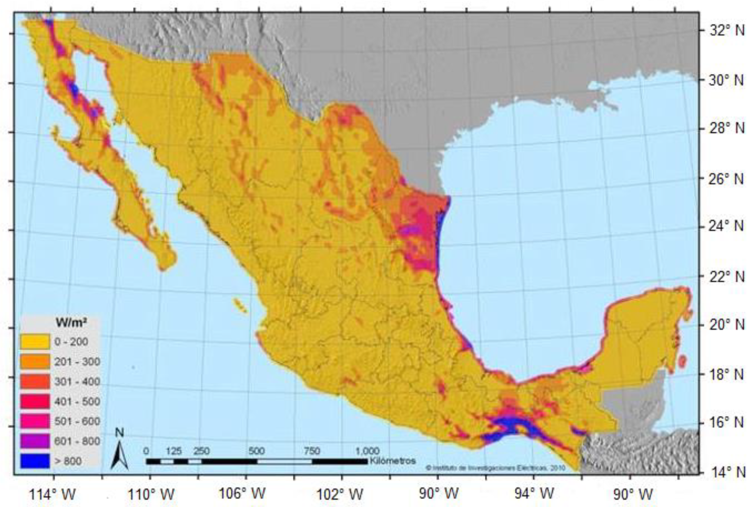
2. Study Location and Measured Data

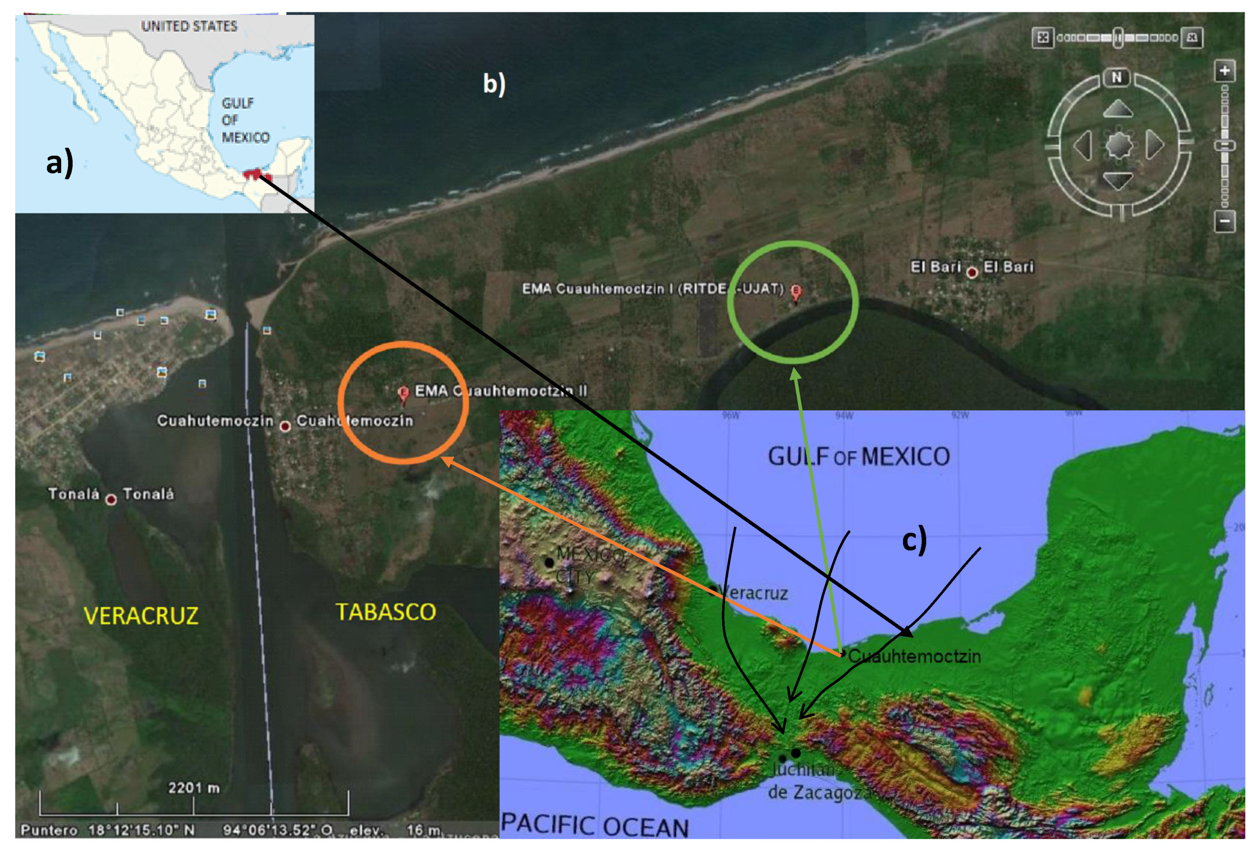
2.1. Specific Site Location

The selected location for weather data acquisition corresponds to the coastal zone of Cuauhtemotzin, Tabasco, Mexico positioned geographically in the north of Tehuantepec Isthmus (latitude: 18 12 15.10 N; longitude: 94 06 13.52 W; height: 16 m.a.s.l). This is located southeast of Mexican country on the border between Tabasco and Veracruz, bounded on the north by the Gulf of Mexico and on the south by La Venta, Oaxaca. This region is characterized by a flat wooded land with vegetation, surrounding trees of medium and high altitude, and hot humid tropic climate.
Cuauhtemotzin represents one of the access point for the virtual trajectory of the wind circulating from the Gulf of Mexico to Pacific Ocean. Figure 2 shows the isotach (lines with equal wind speed in a short or medium distance) extended arbitrarily to indicate the direction of the wind flow that is exchanged in the Tehuantepec Isthmus. As can be seen in the figure, due to the orographic conditions of the south of the Isthmus, this reduces the circulation area of the air coming from the gulf increasing its kinetic energy. This causes the wind circulating in the study zone to have moderate speed but with continuous flow throughout the year.

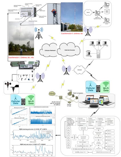
2.2. Experimental System and Instrumentation

To measure climatic data, two wind monitoring towers (Cuauhtemotzin I and Cuauhtemotzin II), were built by Autonomous University Juarez of Tabasco in the study site, separated by 3.8 km. A set of automatic weather stations (AWS) were installed at 33 and 54 m.a.g.l. for Cuauhtemotzin I, and 26 m.a.g.l. for Cuauhtemotzin II. Weather parameters measured were solar irradiation, wind speed, wind direction, ambient temperature, atmospheric pressure, rain precipitation and relative humidity. The sampling period of weather variables was 1 Hz and the records were obtained by arithmetic averages every 10 min. The records were stored in a data logger and managed remotely by Global System for Mobile (GSM) protocol communications. An Internet server was located 160 km away to store the registers in a database, and then process and analyze them.
Climatic datasets collected correspond to a measurements campaign conducted in 2016. Figure 3 illustrates W S trends from the three heights measured, randomly taken from the database for one day (24 h). The figure shows high roughness conditions around the study area given by the low wind speed levels reported at 26 m. On the other hand, the records indicate that the increments of height double the wind speed at 54 m (gain of 50%).

3. Wind Assessment

This section presents the statistical analysis of the wind data measured by the two monitoring towers. Other than that, the influence of climatic variables on wind speed is also studied, as well as the profile of wind speeds for the zone.

3.1. Hellman Power Law

Hellman power law was used to correlate the increment of the wind speed with the increase of the height in the study zone. It is one of the most widespread wind profile models by various organizations to compute the vertical wind increases over a flat terrain [29,30]. Assuming neutral atmospheric conditions, the model is given by:
W S W S 0 = h h 0 α
where W S is the wind speed at height h; W S 0 is the reference wind speed at the reference height h 0 ; and α is the power law index (PLI) determined by the orographic characteristics, surface roughness, mean wind speed, and climatic conditions [31]. Table 1 contains PLI ( α values) for different landscape types reported in literature.
The calculation of this profile is useful to perform approximations of wind speed at a similar height of wind turbine hub height. In the current work, the obtained results were evaluated for a wind turbine (WT) hub height of 54.0 m and cut-in wind speed of ( W S c ) 3.0 m/s [32]. The selected WT is designed to operate in low wind speed regions.

3.2. Wind Distribution Function

The International Standard IEC 61400-12 and other international normatives recommend the use of the Weibull probability distribution function (PDF) to estimate the WE frequency, which is described by the mathematical expression:
f ( W S ) W = k c W S c k 1 e W S c k
where c is the scale parameter, k is the shape parameter, and W S is the wind speed. However, studies carried out at the location of La Venta (south of Tehuantepec Isthmus) indicate that this expression is not adequate to represent the wind regimes in the area [10,33]. According to these studies, a Bimodal PDF provides a better fit to describe the wind behavior for the south of Tehuantepec Isthmus:
f ( W S ) B = A 1 σ 1 2 π exp ( W S μ 1 ) 2 2 σ 1 2 + A 2 σ 2 2 π exp ( W S μ 2 ) 2 2 σ 2 2
It is composed of a linear combination of two weighted Gaussian distribution functions where A 1 and A 2 represent the weight factors, σ 1 and σ 2 are the scale factors established by the standard deviation of the left and right Gaussian distribution, and μ 1 and μ 1 are the factors established by the location of the mean value of the left and right Gaussian distribution.
To identify the PDF model with the best fit performance respect to the wind behavior, a comparison using the statistic measurements coefficient of determination (R 2 ) and Kolmogorov–Smirnov test (SK) was conducted. R 2 is a statistical measure widely used for the evaluation of WS frequency distributions [34,35]. It measures the strength of the linear relationship between the expected and observed frequencies of the bins; the greater is its value (R 2 1), the greater is the fit of the model to the behavior of the probability distribution. On the other hand, SK represents the maximum difference between the cumulative probability of the specified distribution and that of the empirical distribution function calculated [8]. Contrary to R 2 , smaller KS values indicate a better fit between the underlying theoretical distribution and the observed data values.

3.3. Assessment Results
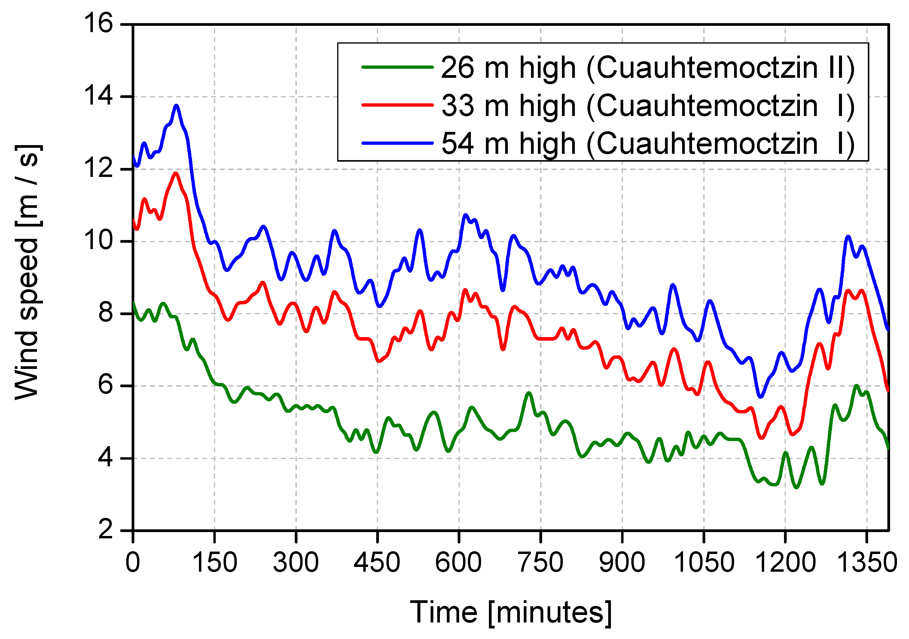
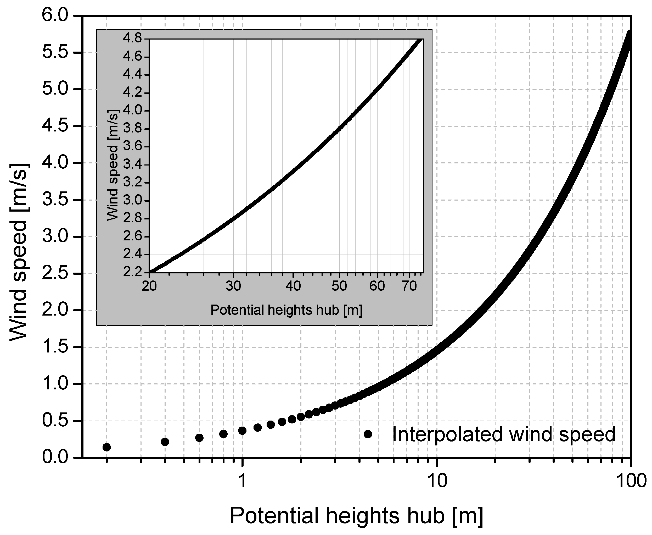
3.3.1. Wind Profile

PLI for Cuauhtemotzin wind profile was calculated and verified by using annual average W S for the three height measured in the zone. Applying Equation (1) an α = 0.5988 was obtained. As can be seen, this value is much higher than those reported in Table 1. This indicates a high roughness in the surrounding terrain, caused by the height of the trees and vegetation in the area (20–40 m.a.g.l.). In addition, studies have shown that PLI is regularly affected by air temperature [36]; therefore, the warm humid climate of the study site also represents an influential factor for the obtained α value. Table 2 contains a comparison of the obtained α with respect to other values reported in the literature. The comparison contemplates the W S estimation at a height of 54 m (m.a.g.l.). As can be appreciated, by increasing PLI value, the estimation error of the W S extrapolated decreases until it reaches 3.41% less than the measured W S using the computed α .
To identify the WR feasibility for Cuauhtemotzin, extrapolated W S α = 0.598 was analyzed with respect to the operating conditions of wind turbine models (WTM) with 54, 50, and 60 m (m.a.g.l.) hub heights, respectively. WTM considered are designed to operate in low wind speed regions [32]. Results in Table 2 show that W S α = 0.598 exceeds the cut-in wind speed ( W S c ) for the three WT models analyzed. Therefore, Cuauhtemotzin location has favorable conditions of operation under the design conditions evaluated. The WS vertical profile obtained in this study is illustrated in Figure 4.

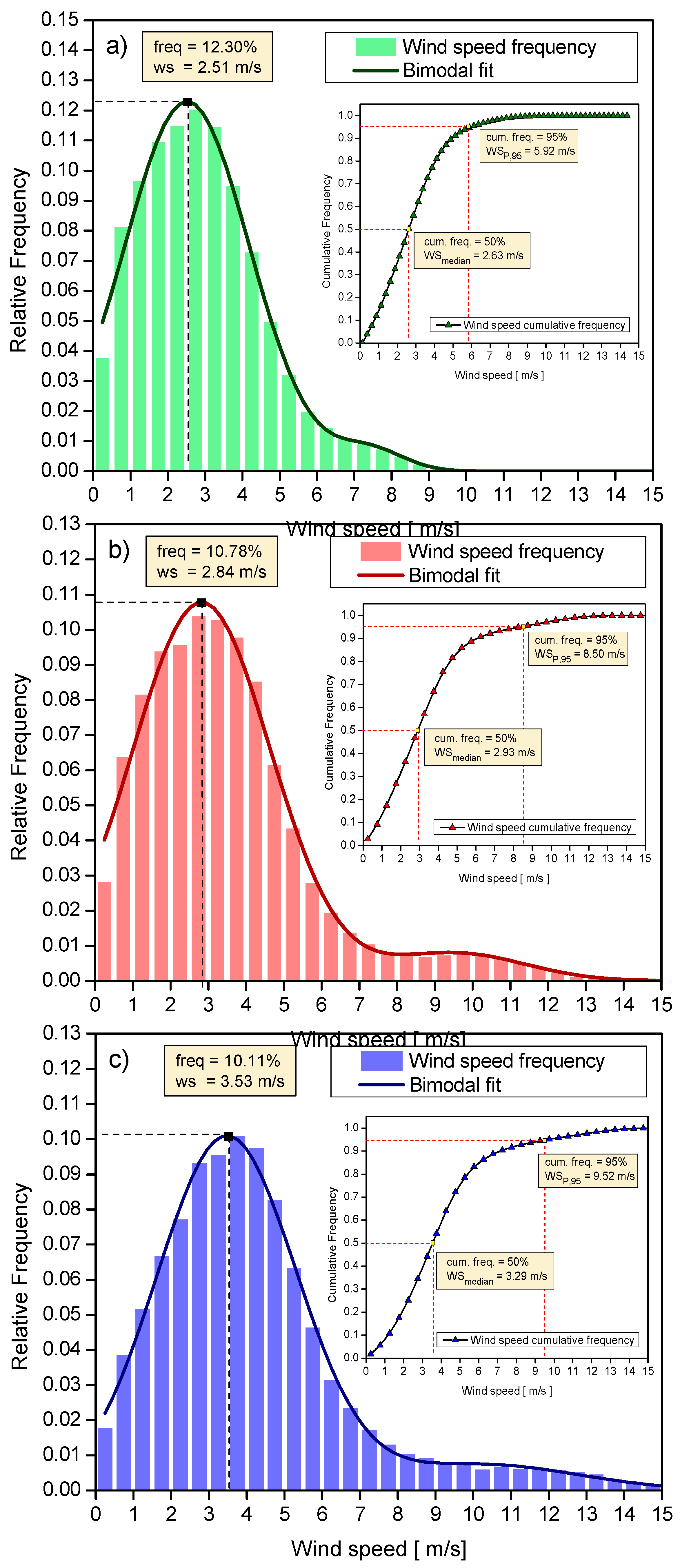
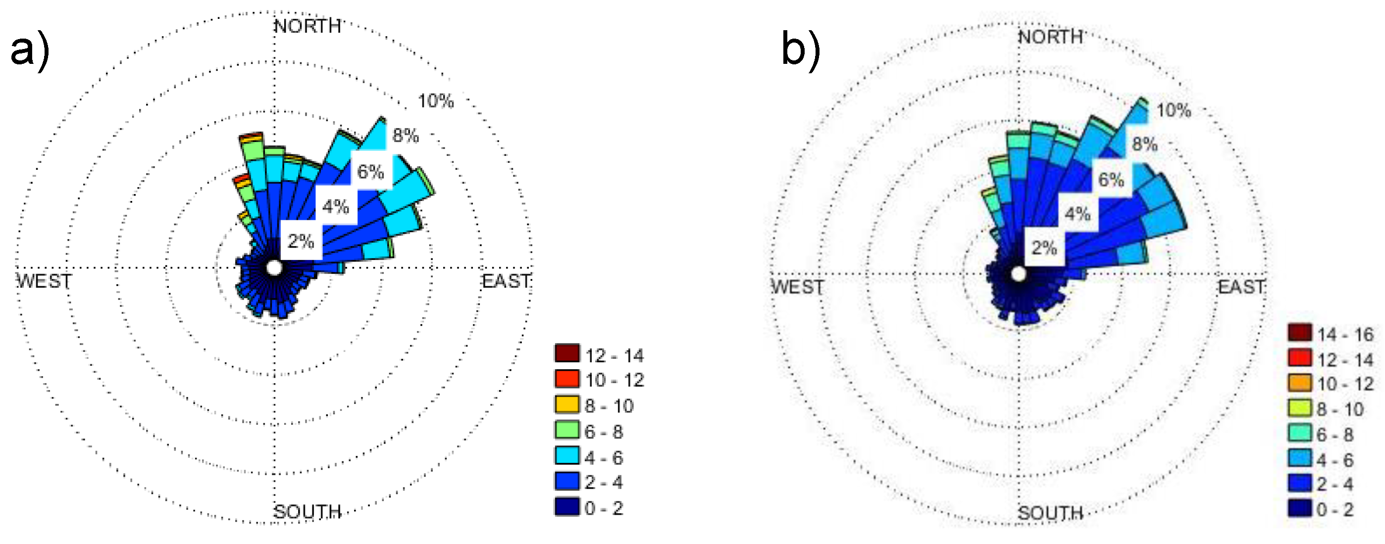
3.3.2. Data Analysis

The statistical results from the analysis of the wind data measured at the study site are summarized in Table 3. From the table, the annual average wind density ( ρ a i r ) reported is 1.17845 kg/m 3 with a standard deviation (Std. Dev.) of 0.01488 kg/m 3 . These variations are caused by the influence of air temperature ( T a ), atmospheric pressure ( P a t m ), and relative humidity ( R H ). The measurements identified that ρ a i r presents an exchange rate of 0.0046 kgm−3 °C−1 for the warm humid tropical climate conditions of the region. Additionally, presences of R H in the air reduces significantly ρ a i r . The statistical results indicate that, for Cuauhtemotzin zone, R H presents a variation of 20% per year with a Std. Dev. ± 8.8614 , being the element with the greatest impact on annual ρ a i r fluctuations. Based on the previous description, annual reports of ρ a i r are lower than the standard value assumed in the literature for the evaluation of the wind potential ( ρ = 1.225 kg/m 3 ). Therefore, the use of the standardized ρ for the location of Cuauhtemotzin underestimates the wind potential for up to 6.3%.
The comparison of the wind probability estimation models presented in Table 4 indicate that Weibull model is not suitable for the description of wind behavior in the area (R 2 < 50% and KS > 0.9). Otherwise, modeling results for bimodal function present R 2 > 99% and KS ≪ 0.1 for the three measured heights, providing great reliability in the models for the estimation of the wind resource. Table 4 also contains the recorded annual average values of wind speed and wind power density (WPD). As can be seen, the Weibull model underestimates the available WPD, which has repercussions on wind turbine operation problems and damages. These results agrees with that reported by Jaramillo et al. [10] where the winds in some coastal areas or sites are bimodal. Therefore, Weibull model, recommended by the International Standard IEC 61400-1, is not appropriate for the evaluation of WR in Tehuantepec Isthmus and specific site with similar characteristics.
Figure 5 shows the relative and cumulative probability density obtained by Bimodal PDF to identify the characteristics of the wind in Cuauhtemotzin. The dominant W S for the measurements at 26, 33, and 54 m (m.a.g.l.) are 2.51 (12.30%), 2.84 (10.78%), and 3.53 m/s (10.11%), respectively. This categorizes the location as a zone with wind class 1 [37]. On the other hand, cumulative frequency graphs provide maximum and minimum useful wind interval for each measured height (between 50% and 95% of the bimodal distribution). According to the aforementioned, the dominant and average speed of the wind (3.53 and 4.12 m/s, respectively) at 54 m are enough to overcome the cutting speed (3.0 m/s), allows the rotation of the generator. In addition, the cumulative frequency at this height shows that the useful wind range is between 3.29 and 9.52 m/s. This indicates very low possibility to reach the rates wind speed ( v r = 12.00 m/s), ensuring an acceptable continuous operation.
According to Figure 6, NE-N is the most dominant and prevalent wind direction in Cuauhtemotzin. Additionally, the wind behavior shows that it has 16 different dominant sections, as listed in Table 5. It was identified that that four of these sections have the highest average W S and frequency. Therefore, separating for this case into two predominant modes for the direction of wind flow—sea–land and land–sea wind—at the site. This coastal dynamic intercalation of the wind agrees with a bimodal behavior where the average wind speed is W S ¯ ≅ 3.2247 ms 1 and the standard deviation between these is σ 0.504 for that address sector, whose neighbourhood of greater frequency are in: NNW, N, ENE, NE and NNE, while for the rest of the directions of the historical wind rose of the site, the W S ¯ 1.4123 ms 1 and the standard deviation is σ 0.339 .

4. Artificial Intelligence Forecasting Modeling

Based on the results presented in the previous section, Cuauhtemotzin has wind conditions of interest for the development of wind projects, from the technical point of view. This makes it feasible for the development of forecasting models. W S forecasting is crucial to improve the operability and optimize the profitability of wind projects. However, given the random and unstable nature of the wind, the development of effective prediction models is very complicated. According to this, an AI approach with global sensitivity analysis (GSA) is presented in this work as an alternative method to forecast the wind resource in a wet humid tropical zone. AI technique used to forecast is the known as Multi-Gene Genetic Programming (MGGP). The prediction horizon considered in this paper corresponds to a very short-term wind forecast with 10-min intervals [38].

4.1. Multi-Gene Genetic Programming Approach

MGGP is a computational technique based on Charles Darwin’s evolution theory used for the modeling of complex non-linear phenomena. MGGP method consists in a set of mathematical expressions randomly generated, which are evaluated and modified iteratively in order to obtain the model with the minimum global error between simulated results and experimental measurements [39].
MGGP iterative modeling process is illustrated in Figure 7. First, the algorithm is initialized by creating a random population of mathematical functions from simple arithmetic operators and independent process variables. Subsequently, the models are ranked according to their performance, discarding the worst models and assigning the best ones for a genetic recombination process. In genetic recombination, the models develop offspring through the modification of genes (mutation or cross-over) in order to generate better mathematical solutions. The new elements are incorporated into the population. The new population is tested again in the algorithm until the number of generations assigned to the process are completed or the minimum tolerable limit of error is reached. The final product is a mathematical equation described by the form:
y ( x ) = H 1 m 1 + H 2 m 2 + H n m n + B
where H are the genes, m is the weight of each gene, B is the bias or offset value, and the subfix n represents the total number of genes for the MGGP model.

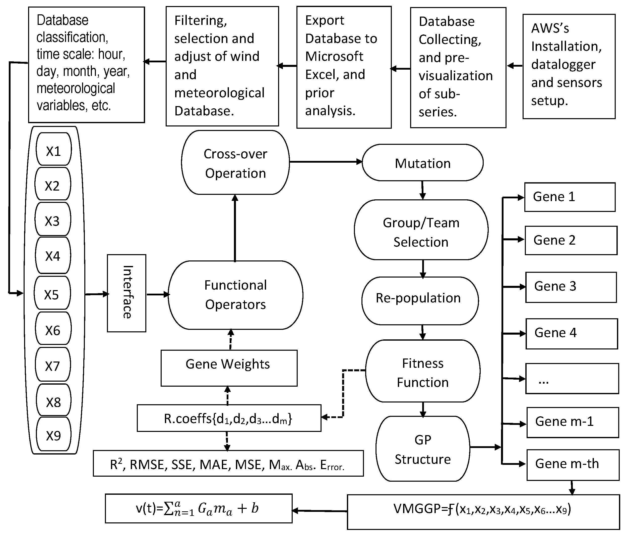
4.2. Computational Methodology

In this work, forecast model considers the influence of climatic variables on the W S behavior. Therefore, the developed model corresponds to a W S time series WITH additional exogenous input variables. To model using the MGGP method, a series of activities are required (Figure 7); these are summarized in the computational methodology described below:
(I) Working database generation. A working database was created by using the atmospheric parameters acquired with the AWS during the measurement campaign from Cuauhtemotzin II. The climatic parameters considered to integrate the database were selected from the cross-correlation analysis presented in Table 3, assuming a relevance threshold >10%. Besides, to know the number of required W S past values for the modeling process, an autocorrelation analysis was performed. The analysis indicates that W S has a strong correlation with respect to four previous measurements. The information of the database used for the modeling process in MGGP is enlisted in Table 6.
(II) Development and evaluation W S forecast models. To perform the modeling, the database was divided into a training section and test section. In the training section (integrated by 80% of the data), the algorithm learns to estimate the results from a function based on samples of real measurements. Then, the best equations are evaluated with the test data (the remaining 20%); this second part has the purpose of determining the feasibility of the model to evaluate data that are not involved in its creation. To obtain a reliable model, several runs for W S forecasting were conducted based on the previously described evolutionary algorithm. The evaluation of multiple runs and different modeling parameters represents a suitable computational strategy to find out the non-linear relationships between the input and output variables.
(III) Statistic analysis. Statistical evaluation was conducted to identify the forecast model with the best accuracy. In the current work, the statistical parameters used are the Mean Percentage Error (MPE) (Equation (5)), Root Mean Squared Error (RMSE) (Equation (6)), and Mean Absolute Error (MAE) (Equation (7)). These parameters correspond to most widely used in the evaluation of predictive models based on AI [22,23,24,25,40]. MPE describes how many the forecasts of a model differ from actual values of the quantity being forecast. MPE is expressed mathematically as:
M P E = 1 a i = 1 a ( W S E x p W S M G G P ) W S E x p × 100
where a represent the number of samples per set, W S E x p is the measured WS and W S M G G P is the forecasted W S . The RMSE determines the accuracy of the model comparing the deviation of simulated and experimental values:
R M S E = 1 a i = 1 a W S E x p W S M G G P 2
High values of RMSE indicate high error margins in the forecasts, while values very close to zero indicate predictions with high accuracy. The MAE is useful to identify the mean error value between the observed and adjusted series. Similar to the RMSE, the best forecast models are found in the values closest to zero. It is given by the expression:
M A E = 1 a i = 1 a | W S E x p W S M G G P |
Besides, the coefficient of determination (R) is another adjusted time series parameter that shows the relationship of the predicted data with the measured data:
R = i = 1 N W S E x p W S ¯ E x p W S M G G P W S ¯ M G G P i = 1 N W S E x p W S ¯ E x p 2 W S M G G P W S ¯ M G G P 2
where ( W S ¯ ) is the average of W S . According to this parameter, values close to 1 indicate very precise correlations, values higher than 0.75 indicate a good performance of the model, and values lower than 0.5 show that the predictions of the model are not adequate.

4.3. Sensitivity Analysis

Sensitivity analysis determines the relative importance of the M input variables of a mathematical model x i = x 1 , x 2 , , x M with respect to its output response y k . Due to the heuristic nature of AI-based models, sensitivity analysis is a necessary process to determine the adaptation of the system to the phenomenon studied [41]. In a sensitivity analysis, the greater is the disturbance in the output of the model, the greater is the influence of the evaluated variable. In the present work, Effective Elements Test (EET) was used [42]. EET is a global sensitivity analysis with low computation time, which ranks the importance of the input variables in a simple way by using the so-called Effective Elements (EEs). These characteristics make it suitable for the analysis of renewable energies’ complex computational models based on AI.
EET works under the concepts of random sampling and One-factor-At-Time (OAT) to compute the EEs. The first one is based on the generation of r random samples for each input variable by using the Latin Hypercube method. In the second one, for each set of input variables x i = x 1 , x 2 , , x M , perturbations are induced by varying one input factor at a time and keeping the other variables fixed. This alteration produces a total of M r + 1 datasets evaluated in the MGGP model. In general, it can be indicated that the EE of the ith input factor x i at a given baseline point x j and for a predefined perturbation is given by [43]:
E E i j = y k x 1 j , x 2 j , x 3 j , , x i j + , , x M j y k x 1 j , x 2 j , x 3 j , , x i j , , x M j
The EEs quantify how much the MGGP result is affected by the disturbance in the ith variable, where the total number of EEs per each variable is r. The mean of the absolute values of EEs μ i * is considered the sensitivity measure for the ith input parameter:
μ i * = 1 r j = 1 r | E E i j |
Sensitivity can be expressed as a percentage if the sensitivity indices obtained by Equation (10) meet the convergence criteria (convergence of sensitivity index, ranking, and screening) described by Sarrazin et al. [44]. Therefore, we defined the percentage value of the sensitivity as:
S i = U i i = 1 M U i
where U i represents the normalized mean of the EEs given as the ratio between μ i * and the maximum value of the mean EEs across all the input factors. On the other hand, as a secondary product, the interaction of the ith input parameter with respect other input parameter can be interpreted from the standard deviation of EEs σ i :
σ i = 1 r j = 1 r | E E i j μ i |

4.4. Forecast Model Results

4.4.1. Multi-Gene Genetic Programming Model

MGGP modeling is influenced by several parameters, affecting the generalization capability of the algorithm. To achieve a minimum prediction error, the model must be subjected to a series of configuration settings. The main parameters that influence the modeling process are the size of the population, the number of genes, the number of generations, the gene tree depth, the set of mathematical functions, the range of the constants, the tournament size, and mutation and reproduction rate. Table 7 enlists the parameter settings used in this work that offer the best accuracy in the shortest computational time possible; its values were obtained by a trial and error approach. Modeling process was conducted using the Matlab software and the GPTIPS 2.0 computational package [45].
To obtain the model that achieve the best fitness for training and testing data, various MGGP runs were performed. The values of the statistical parameters (RMSE, MAE, and MPE) closer to zero assure a better forecasting accuracy. Similarly, R results higher than 0.75 are considered good; R values of 0.36–0.75 indicate a acceptable performance, and R values <0.36 are considered unacceptable. Statistical results for the best W S forecast computational model are presented in Table 8. As can be appreciated, the statistical indicators show that the model generated with MGGP has good approximations for the estimation of the wind speed in a 10-min interval. Similar statistical ranges have been reported by Cadenas et al. [28] and do Nascimento Camelo et al. [40] for hourly forecasts in Mexico and Brazil, respectively. Moreover, the statistical indicators for both the training and testing phases have similar values, which shows the representativeness of the model with respect to the phenomenon. Consequently, these results indicate that the model is capable of making predictions with a very adequate range of certainty.
Additionally, Table 8 presents a comparison of the model obtained with one of the most widely used models in predictions of time series such as the autoregressive integrated moving average model (ARIMA). From this comparison, it is observable that the prediction approach based on evolutionary programming estimates the wind behavior statistically better than ARIMA for a very short period of forecast, such as the one presented in this work (10-min interval). This indicates the competitiveness of the MGGP to be applied as a tool in the prediction of wind behavior and allows its incorporation as an alternative to the existing computational techniques for wind speed forecasting.
Viability of the developed model was analyzed by an autocorrelation study of prediction errors, as presented in Figure 8. As can be seen in the figure, the autocorrelations of the training and test data do not present perceptible patterns within a significant limit of 95%. Therefore, the errors obtained are due to the random behavior of the irregularities in the time series.

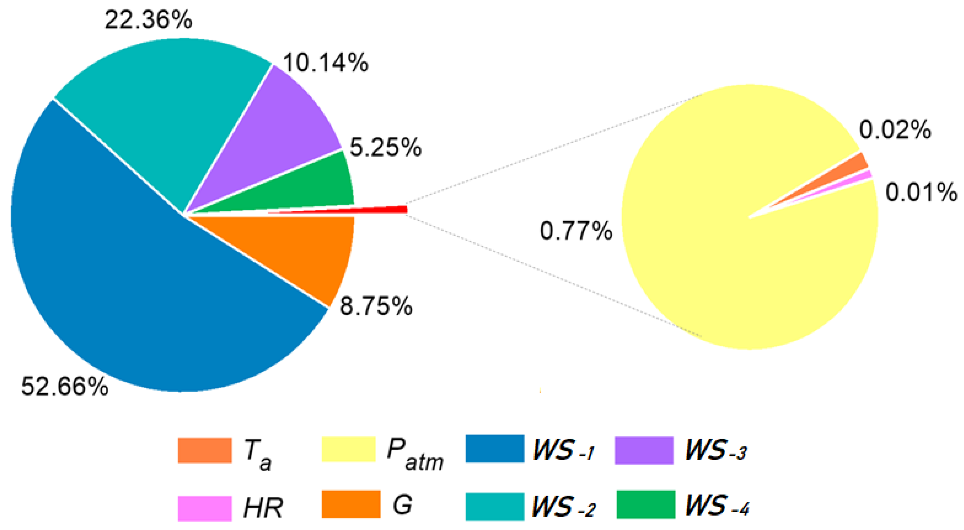
4.4.2. Sensitivity Analysis Evaluation

Sensitivity analysis was conducted using a sample strategy based on Latin Hypercube, a uniform distribution function for random samples generation, and a maximum number of evaluated samples r equal to 500 per each input variable. All calculations were executed using the MATLAB toolbox SAFE 1.1 [46]. According to the results, the evaluation complied with the convergence criteria using the normalized sensitivity indexes, making feasible the presentation of results in percentage form.
Figure 9 illustrates the influence for each input variables of analyzed mathematical model. According to the results of the sensitivity analysis, the model perceives that greatest impact on the prediction of wind speed is given by W S 1 with 52.66% followed by W S 2 with 22.36%, W S 3 with 10.14%, G with 8.75%, and W S 4 with 5.25%. On the contrary, the least influential variables were atmospheric pressure, air temperature and relative humidity, with 0.77%, 0.02%, and 0.01%, respectively. These results are in accordance with the indicated by the autocorrelation analysis (Section 4.2), where four previous W S data play an important role in the forecast of the future value to 10 min. On the other hand, the discrepancy between the exogenous variables used and the influence reported in Table 2 is given by the reduced change gradient that these parameters present in the 10-min interval. Similar results were reported by Cadenas et al. [28] for the north of Tehuantepec Isthmus, where four previous W S measurements and G were identified as the most influential parameters to W S forecast with one-hour intervals. The above provides a correlation of wind phenomena between the north and south of Tehuantepec Isthmus, expanding the landscape of the evaluation of the resource for the zone.
These results give the certainty to the developed model through evolutionary programming of being able to interpret the physical behavior of the phenomenon, despite being constructed by stochastic processes. Table 9 summarizes the information regarding the degree of interaction of each input variable with the others. As can be seen, the parameters that most influence the others are W S 1 , W S 2 and G. The high influence of the immediate past WS values is due to the nature of the time series, where the previous values are highly correlated with each other in order to carry out the estimation. However, this dependence is reduced as it projects back the past, which is demonstrated by the reduced influence of W S 4 . On the other hand, the influence of G is due to the relevance that this variable has on the various meteorological phenomena of the Earth, among them the WS. In general, with the exception of W S 4 , the influence exerted by the input variables between them is very similar to their impact on the output of the developed model.
The results presented in the sensitivity analysis allowed determining that the predictive model based on multi-genetic programming is perfectly adapted to the physical behavior of the wind governed by a series of time. In addition, the interaction results between input variables guarantee what is specified by the autocorrelation, where four previous WS values are enough to forecast the next value.

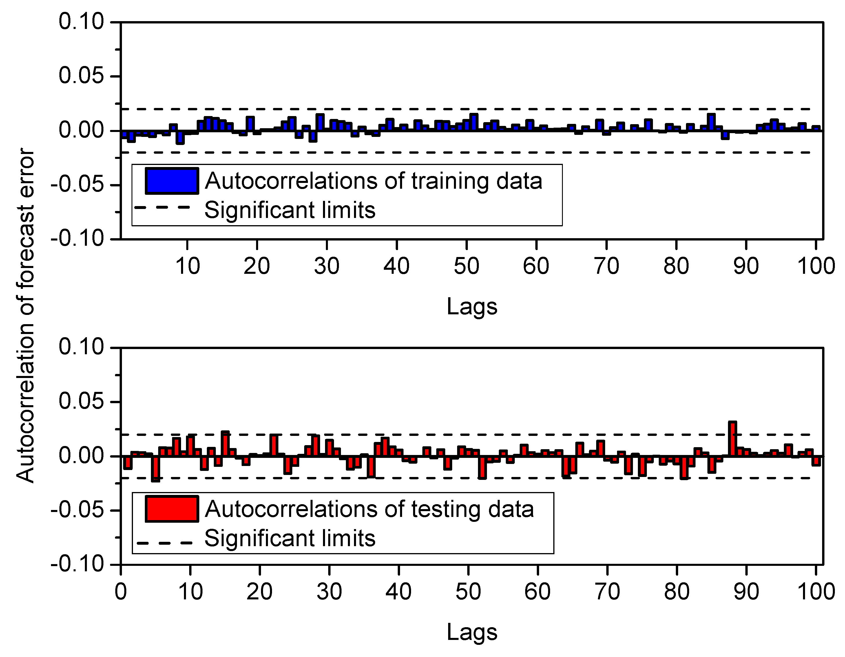
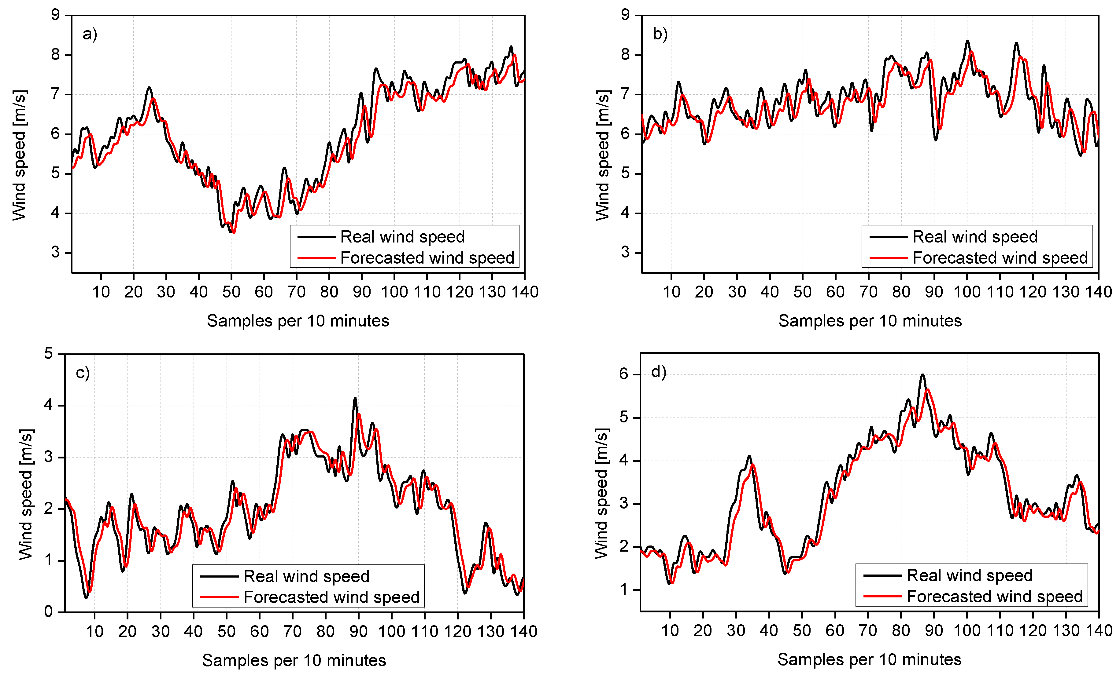
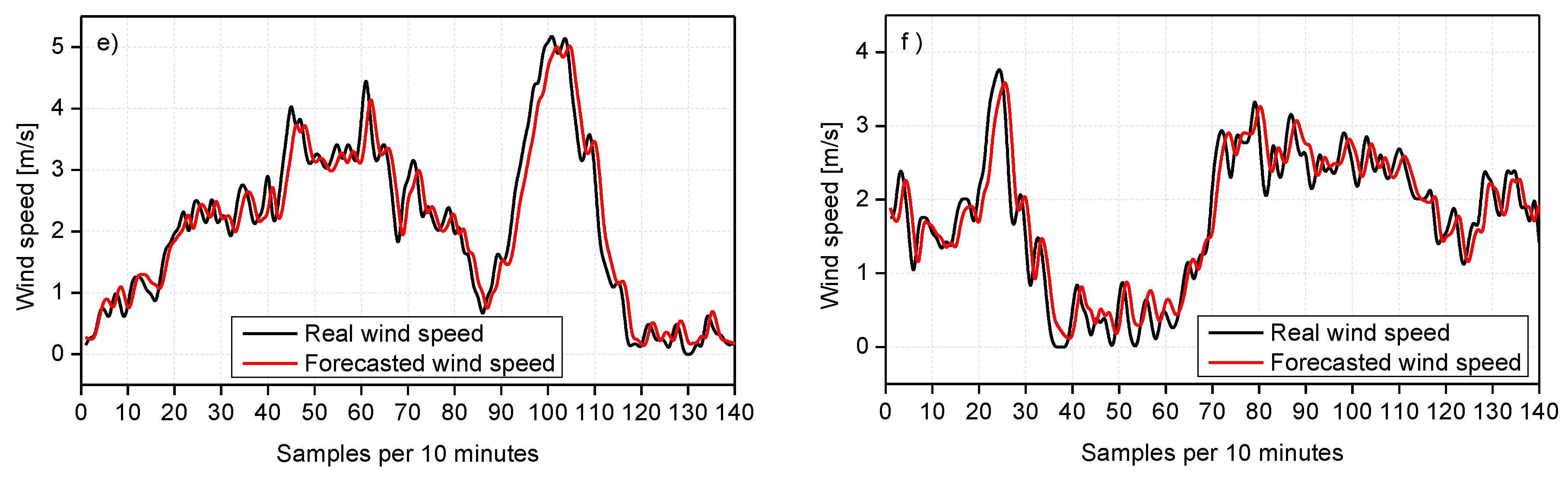
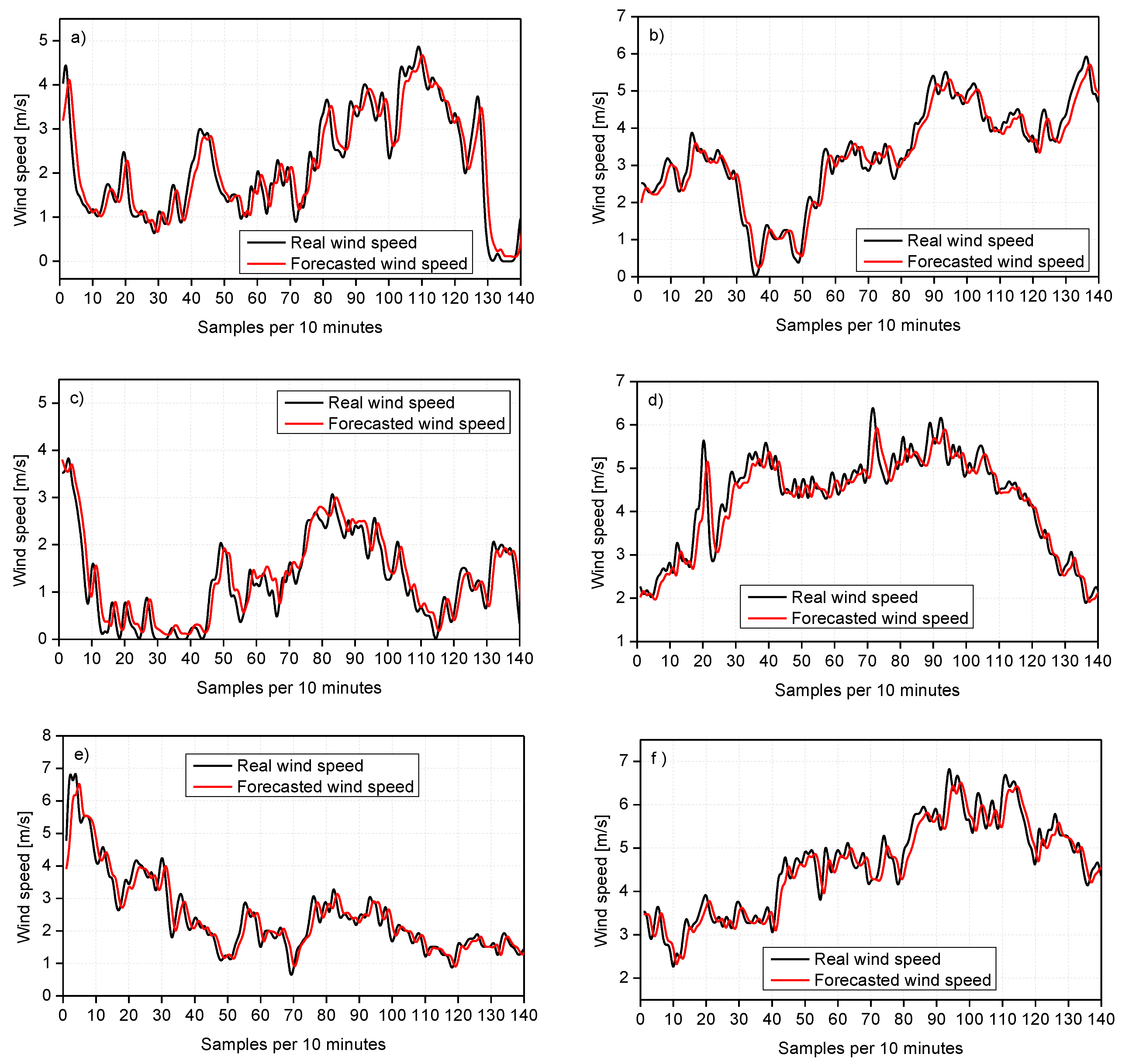
4.4.3. MGGP Forecast Model Validation

The performance of the MGGP model is validated by a comparison between measured wind values and forecast results by using data not involved in the training and testing phase. To fully appreciate the time series behavior, the evaluation was carried out using measurements corresponding to a full day of each month. In Figure 10 and Figure 11, the forecast system based on MGGP is subjected to different prediction conditions throughout the year, in which it adapts adequately to variations and sudden changes of the wind. The evaluation demonstrates that MGGP model provides a good approach of W S behavior in 10-min intervals during the 12 months of the year. On the other hand, it is observed that the most of forecast errors present values lower than the real one, indicating that the predictions do not over estimate the wind’s energy potential for the area.
It is important to note that since the period of prediction is for the 10 min immediately after, the computation time is irrelevant. For this work, all the predictive calculations were carried out in a period of less than one minute, which provides a wide margin for very short-term decision making. Therefore, the developed model represents the first forecasting approach and a feasible alternative for the very short-term estimation of W S for Cuauhtemotzin location. Both the statistical results and the evaluation of the model showed that it has an acceptable prediction accuracy. Then, the forecasting methodology presented in this work represents an important auxiliary tool for estimating the energy potential of the region, and the results can be extrapolated to different heights under the appropriate considerations.

5. Conclusions

Tehuantepec Isthmus is one of the areas with greatest wind power potential around the world. However, although there is extensive documentation on wind’s characteristic and behavior for the southern zone of the isthmus, there are no studies that complement the region’s energetic panorama for the northern zone. In that sense, this work addressed the wind resource assessment and wind speed forecast for Cuauhtemotzin, Mexico, located at north of the Tehuantepec Isthmus. The study was conducted using climatic data: wind speed, wind direction, solar radiation, air temperature, relative humidity, rain precipitation, and atmospheric pressure measured at 26, 33, and 54 m.a.g.l.
The measurements allowed us to develop the profile of wind speeds for the zone, identifying which external parameters such as temperature, humidity and pressure affect the behavior of the wind. The evaluation of the resource indicated that the dominant wind direction for the area is between the north-northwest and north-northeast (wind flow sea–land) with an annual frequency probability greater than 90%, which have wind speeds higher than average according to the records. In addition, it was also identified that the wind probability distribution cannot be represented under the Weibull model recommended by International Standard IEC 61400-1. The analysis shows that the wind behavior for the region is adapted to a bimodal probability fitting, with an accuracy greater than 99%. These results are similar to those reported in the southern region of Tehuantepec Isthmus. Hence, Weibull probability distribution function is not appropriate for the wind resource assessment in the wind corridor formed in the Isthmus.
On the other hand, the application of a new approach for the prediction of wind speed based on an evolutionary programming is presented. From a computational methodology, a time series exogenous model was developed to forecast wind speed in 10-min intervals, using multi-gene genetic programming and global sensitivity analysis. Forecast model considered the four previous values of the wind speed and as exogenous parameters the solar radiation, air temperature, atmospheric pressure, and relative humidity. The model’s statistical parameters (R = 0.9567, MPE = −13.58, RMSE = 0.5287, 0.38831) demonstrated a good precision in the estimation of the wind speed, and the autocorrelation errors indicate the absence of patterns that compromise its viability of use. In addition, sensitivity analysis results show that the most influential parameters for forecasting were the previous values of wind speed and solar radiation. A similar dependence was identified for the south of Tehuantepec Isthmus. This results provides a correlation of the wind phenomena between the north and south zones, expanding the landscape of the evaluation for the resource.
Finally, this work presented the analysis for a case study in Mexico; however, the methodology developed is useful to complete the wind energy scenario in locations with similar geographical conditions around the world. Moreover, it has been shown that multi-gene genetic programming is an effective technique for the prediction of wind speed, enriching the catalog of computational tools suitable for the development of wind forecast models. Thus, the presented methodology and computational approach can be implemented to evaluate the wind resource in different regions.

Author Contributions

L.M.L.-M., E.V.M.-M., and K.M.A.-C. conceived and designed the experiments; L.M.L.-M. and I.H.-P. performed the experiments; L.M.L.-M., M.-M.E., and A.B. analyzed the data; O.M.T. contributed reagents/materials/analysis tools; and L.M.L.-M. and O.M.T. wrote the paper.

Funding

Universidad Juárez Autónoma de Tabasco: 12219. Fonde SENER-Sustentabilidad 254667.

Acknowledgments

The authors thank Universidad Juárez Autónoma de Tabasco Funding sources and LERMER (Laboratorio de Energías Renovables y Mediciones Estrategias Renovables) for the use of their Automatic Weather Stations and equipment in this research and to federal funds number 12219, program PFCE project number 20180977 for supporting research collaboration stances in UADY, Merida Yuc. The authors also thank Hector Pastrana Alcocer and Rasikh Tariq for their support in the modeling face and language revision, respectively.

Conflicts of Interest

The authors declare no conflict of interest. Authors declare any personal circumstances or interest that may be perceived as inappropriately influencing the representation or interpretation of reported research results. Any role of the funding sponsors in the design of the study; in the collection, analyses or interpretation of data; in the writing of the manuscript, or in the decision to publish the results. There is no role. The founding sponsors had no role in the design of the study; in the collection, analyses, or interpretation of data; in the writing of the manuscript, and in the decision to publish the results.

References

  1. REN21. Renewables 2017: Global Status Report; Technical Report; Renewable Energy Policy Network for the 21st Century: Paris, France, 2017. [Google Scholar]
  2. IEA. Renewables Information: Overview; Technical Report; International Energy Agency: Paris, France, 2018. [Google Scholar]
  3. Pérez-Denicia, E.; Fernández-Luqueño, F.; Vilariño-Ayala, D.; Manuel Montaño-Zetina, L.; Alfonso Maldonado-López, L. Renewable energy sources for electricity generation in Mexico: A review. Renew. Sustain. Energy Rev. 2017, 78, 597–613. [Google Scholar] [CrossRef]
  4. Hernández-Escobedo, Q.; Perea-Moreno, A.J.; Manzano-Agugliaro, F. Wind energy research in Mexico. Renew. Energy 2018, 123, 719–729. [Google Scholar] [CrossRef]
  5. Guerrero, A.L. CEMIE-EOLICO, Alianza Para la Ciencia y Tecnología del Viento; Technical Report; CEMIE Eólico, Instituto Nacional de Electricidad y Energías Limpias: Cuernava, Mexico, 2016.
  6. Alemán-Nava, G.S.; Casiano-Flores, V.H.; Cárdenas-Chávez, D.L.; Díaz-Chavez, R.; Scarlat, N.; Mahlknecht, J.; Dallemand, J.F.; Parra, R. Renewable energy research progress in Mexico: A review. Renew. Sustain. Energy Rev. 2014, 32, 140–153. [Google Scholar] [CrossRef]
  7. Hau, E. Wind Turbines; Springer: Berlin/Heidelberg, Germany, 2013. [Google Scholar]
  8. Zhou, J.; Erdem, E.; Li, G.; Shi, J. Comprehensive evaluation of wind speed distribution models: A case study for North Dakota sites. Energy Convers. Manag. 2010. [Google Scholar] [CrossRef]
  9. Gräbner, J.; Jahn, J. Optimization of the distribution of wind speeds using convexly combined Weibull densities. Renew. Wind. Water Sol. 2017, 4, 7. [Google Scholar] [CrossRef]
  10. Jaramillo, O.A.; Borja, M.A. Wind speed analysis in La Ventosa, Mexico: A bimodal probability distribution case. Renew. Energy 2004. [Google Scholar] [CrossRef]
  11. Erdem, E.; Shi, J. ARMA based approaches for forecasting the tuple of wind speed and direction. Appl. Energy 2011. [Google Scholar] [CrossRef]
  12. Wang, J.; Song, Y.; Liu, F.; Hou, R. Analysis and application of forecasting models in wind power integration: A review of multi-step-ahead wind speed forecasting models. Renew. Sustain. Energy Rev. 2016, 60, 960–981. [Google Scholar] [CrossRef]
  13. Okumus, I.; Dinler, A. Current status of wind energy forecasting and a hybrid method for hourly predictions. Energy Convers. Manag. 2016, 123, 362–371. [Google Scholar] [CrossRef]
  14. Nowotarski, J.; Weron, R. Recent advances in electricity price forecasting: A review of probabilistic forecasting. Renew. Sustain. Energy Rev. 2018, 81, 1548–1568. [Google Scholar] [CrossRef]
  15. Archer, C.L.; Vasel-Be-Hagh, A.; Yan, C.; Wu, S.; Pan, Y.; Brodie, J.F.; Maguire, A.E. Review and evaluation of wake loss models for wind energy applications. Appl. Energy 2018, 226, 1187–1207. [Google Scholar] [CrossRef]
  16. Zhang, Y.; Wang, J. A distributed approach for wind power probabilistic forecasting considering spatiooral correlation without direct access to off-site information. IEEE Trans. Power Syst. 2018. [Google Scholar] [CrossRef]
  17. Nielsen, H.A.; Madsen, H.; Nielsen, T.S. Using quanti le regression to extend an existing wind power forecasting system With probabilistic forecasts. Wind Energy 2006. [Google Scholar] [CrossRef]
  18. Pinson, P.; Kariniotakis, G. Conditional Prediction Intervals of Wind Power Generation. IEEE Trans. Power Syst. 2010. [Google Scholar] [CrossRef] [Green Version]
  19. Liu, H.; Shi, J.; Erdem, E. An integrated wind power forecasting methodology: Interval estimation of wind speed, operation probability of wind turbine, and conditional expected wind power output of a wind farm. Int. J. Green Energy 2013. [Google Scholar] [CrossRef]
  20. Zhang, Y.; Wang, J. K-nearest neighbors and a kernel density estimator for GEFCom2014 probabilistic wind power forecasting. Int. J. Forecast. 2016. [Google Scholar] [CrossRef]
  21. Palit, A.K.; Popovic, D. Computational Intelligence in Time Series Forecasting; Springer: Berlin, Germany, 2005. [Google Scholar]
  22. Cruz May, E.; Ricalde, L.J.; Atoche, E.J.R.; Bassam, A.; Sanchez, E.N. Forecast and Energy Management of a Microgrid with Renewable Energy Sources Using Artificial Intelligence. In Intelligent Computing Systems. ISICS 2018. Communications in Computer and Information Science; Brito-Loeza, C., Espinosa-Romero, A., Eds.; Springer International Publishing: Berlin, Germany, 2018; pp. 81–96. [Google Scholar]
  23. Zendehboudi, A.; Baseer, M.; Saidur, R. Application of support vector machine models for forecasting solar and wind energy resources: A review. J. Clean. Prod. 2018, 199, 272–285. [Google Scholar] [CrossRef]
  24. Zhang, F.; Dong, Y.; Zhang, K. A Novel Combined Model Based on an Artificial Intelligence Algorithm—A Case Study on Wind Speed Forecasting in Penglai , China. Sustainability 2016, 8, 555. [Google Scholar] [CrossRef]
  25. Li, G.; Shi, J.; Zhou, J. Bayesian adaptive combination of short-term wind speed forecasts from neural network models. Renew. Energy 2011. [Google Scholar] [CrossRef]
  26. Hocaoglu, F.O.; Gerek, Ö.N.; Kurban, M. A novel wind speed modeling approach using atmospheric pressure observations and hidden Markov models. J. Wind Eng. Ind. Aerodyn. 2010. [Google Scholar] [CrossRef]
  27. Cortés Pérez, E.; Nuñez Rodríguez, A.; Moreno De La Torre, R.E.; Lastres Danguillecourt, O.; Dorrego Portela, J.R. Forecasting of Wind Spedd with a Backpropagation Artificial Neural Network in the Isthmus of Tehuantepec Region in the State of Oaxaca, Mexico. Acta Univ. 2012, 22, 62–68. [Google Scholar]
  28. Cadenas, E.; Rivera, W.; Campos-Amezcua, R.; Cadenas, R. Wind speed forecasting using the NARX model, case: La Mata, Oaxaca, México. Neural Comput. Appl. 2016, 27, 2417–2428. [Google Scholar] [CrossRef]
  29. ABS. Guide for Building and Classing Floating Offshore Wind Turbine Installations; Technical Report; American Bureau of Shipping: Houston, TX, USA, 2015. [Google Scholar]
  30. Van der Tempel, J.; Diepeveen, N.F.B.; Cerda Salzmann, D.J.; de Vries, W.E. Design of Support Structures for Offshore Wind Turbines. In Wind Power Generation and Wind Turbine Design; WIT Press: Southampton, UK, 2006. [Google Scholar]
  31. Liu, Y.; Chen, D.; Yi, Q.; Li, S. Wind profiles and wave spectra for potential wind farms in South China Sea. Part I: Wind speed profile model. Energies 2017, 10, 125. [Google Scholar] [CrossRef]
  32. Dong, Y.; Wang, J.; Jiang, H.; Shi, X. Intelligent optimized wind resource assessment and wind turbines selection in Huitengxile of Inner Mongolia, China. Appl. Energy 2013. [Google Scholar] [CrossRef]
  33. Jaramillo, O.; Borja, M. Bimodal versus Weibull Wind Speed Distributions: An Analysis of Wind Energy Potential in La Venta, Mexico. Wind Eng. 2004. [Google Scholar] [CrossRef]
  34. Li, M.; Li, X. MEP-type distribution function: A better alternative to Weibull function for wind speed distributions. Renew. Energy 2005. [Google Scholar] [CrossRef]
  35. Kantar, Y.M.; Usta, I. Analysis of wind speed distributions: Wind distribution function derived from minimum cross entropy principles as better alternative to Weibull function. Energy Convers. Manag. 2008. [Google Scholar] [CrossRef]
  36. Albani, A.; Ibrahim, M.Z. Wind Energy Potential and Power Law Indexes Assessment for Selected Near-Coastal Sites in Malaysia. Energies 2017, 10, 307. [Google Scholar] [CrossRef]
  37. Chowdhury, S.; Mehmani, A.; Zhang, J.; Messac, A. Market suitability and performance tradeoffs offered by commercialwind turbines across differingwind regimes. Energies 2016, 9, 352. [Google Scholar] [CrossRef]
  38. Zhang, Y.; Wang, J.; Wang, X. Review on probabilistic forecasting of wind power generation. Renew. Sustain. Energy Rev. 2014, 32, 255–270. [Google Scholar] [CrossRef]
  39. Handbook of Genetic Programming Aplications; Number 2015945115; Springer International Publishing Switzerland: Cham, Switzerland, 2015.
  40. Do Nascimento Camelo, H.; Lucio, P.; Junior, J.; de Carvalho, P. A hybrid model based on time series models and neural network for forecasting wind speed in the Brazilian northeast region. Sustain. Energy Technol. Assess. 2018, 28, 65–72. [Google Scholar] [CrossRef]
  41. May Tzuc, O.; Bassam, A.; Mendez-Monroy, P.E.; Sanchez Dominguez, I. Estimation of the operating temperature of photovoltaic modules using artificial intelligence techniques and global sensitivity analysis: A comparative approach. J. Renew. Sustain. Energy 2018, 10, 033503. [Google Scholar] [CrossRef] [Green Version]
  42. Morris, M. Factorial sampling plans for preliminary computational experiments. Technometrics 1991, 9, 161–164. [Google Scholar] [CrossRef]
  43. Lee, L.; Srivastava, P.K.; Petropoulos, G.P. Overview of Sensitivity Analysis Methods in Earth Observation Modeling; Elsevier Inc.: Amsterdam, The Netherlands, 2017; pp. 3–24. [Google Scholar]
  44. Sarrazin, F.; Pianosi, F.; Wagener, T. Global Sensitivity Analysis of environmental models: Convergence and validation. Environ. Model. Softw. 2016, 79, 135–152. [Google Scholar] [CrossRef]
  45. Handbook of Genetic Programming Applications; Chapter GPTIPS 2: An Open-Source Software Platform for Symbolic Data Mining; Springer Publishing International: Berlin, Germany, 2015.
  46. Pianosi, F.; Sarrazin, F.; Wagener, T. A Matlab toolbox for Global Sensitivity Analysis. Environ. Model. Softw. 2015, 70, 80–85. [Google Scholar] [CrossRef]
Figure 1. Wind power density at 80 m.a.g.l. for the territory of Mexico [6].
Energies 11 03197 g001
Figure 2. Location map: (a) the location for Tabasco State; (b) zoom of masts in Cuauhtemotzin (I and II) in municipality of Cardenas; and (c) location and isotach of Cuauhtemotzin site inside orography trajectory to La Venta, Oaxaca showing proximity in latitude and longitude.
Energies 11 03197 g002
Figure 3. Sample of wind speeds recorded in Cuauhtemotzin zone for the study heights (26, 33, and 54 m).
Energies 11 03197 g003
Figure 4. Cuauhtemotzin wind profile obtained from the measurement campaigns conducted in 2016.
Energies 11 03197 g004
Figure 5. Bimodal distribution for the wind speeds obtained in the measurement campaign: (a) 26 m (Cuauhtemotzin II); (b) 33 m (Cuauhtemotzin I); and (c) 54 m (Cuauhtemotzin I).
Energies 11 03197 g005
Figure 6. Wind direction from the annual measuring campaign in 2016: (a) wind measurements from Cuauhtemotzin I; and (b) wind measurements from Cuauhtemotzin II.
Energies 11 03197 g006
Figure 7. Computational methodology applied to generate the W S forecasting model.
Energies 11 03197 g007
Figure 8. Autocorrelation function of the forecast errors for the MGGP with significant limits of 95%.
Energies 11 03197 g008
Figure 9. Sensitivity analysis results for the forecasting multi-gene genetic programming developed model.
Energies 11 03197 g009
Figure 10. Comparison between experimental WS and simulated values for the first semester of the year (a) January; (b) February; (c) March; (d) April; (e) May; and (f) June.
Energies 11 03197 g010aEnergies 11 03197 g010b
Figure 11. Comparison between experimental WS and simulated values for the second semester of the year: (a) July; (b) August; (c) September; (d) October; (e) November; and (f) December.
Energies 11 03197 g011
Table 1. PLI values according to landscape type.
Landscape α
Flat land with ice or grass0.08–0.12
Sea and coasts0.14
Little hilly areas0.13–0.16
Rural zones0.20
Rugged terrains and forests0.20–0.26
Very rugged terrains and cities0.25–0.40
Table 2. Comparison and evaluation of the wind profile for Cuauhtemotzin considering implementation cases at different heights.
ParametersMeasured α = 0.140 α = 0.143 α = 0.200 α = 0.260 α = 0.400 α = 0.598
WS [m/s]4.122.84582.85202.97343.10673.44143.9796
Error [-]-0.30930.30780.27830.24600.16470.0341
WTMh [m] WS c [m/s] WS r [m/s] WS α = 0.598 [m/s]
Gamesa G58-850543.012.03.9796
Unison U54-750603.012.04.2387
Dewind D4/48-600703.012.04.6486
Table 3. Statistical parameters results of climatic annual variations for for Cuauhtemotzin, Mexico.
VariableUnitsmin.max.meanStd DevWS Cross Corr %
Air temperature( T a )[ C]12.89639.42026.1582.962611.13%
Atmospheric Pressure( P a t m )[mbar]998.451027.551011.354.0508721.91%
Relative Humidity( R H )[%]37.810086.39408.861430.53%
Wind Direction( W D )[ Deg]0355.2125.0309112.59715.6566%
Air Density( ρ a i r )[kgm 3 ]1.122741.242061.178450.014881.6011%
Solar Radiation( S R )[Wm 2 ]0.61276.90198.3771295.975818.9817%
Rain( R n )[mm]022.610.0440.461548.641%
Table 4. PDF models fit comparison for the estimation of wind resource probability in Cuauhtemotzin.
Weibull PDF
h [m]ckR2KSWS [m/s]WPD [W/m 2 ]
266.16061.19350.41070.95642.8353.26
336.96701.20750.34260.95213.4394.83
547.53461.30350.22470.92424.12144.17
Bimodal PDF
h [m]A 1 A 2 σ 1 σ 2 μ 1 μ 2 R 2 KSWS [m/s]WPD [W/m 2 ]
260.01670.51760.92011.67917.38742.51560.94430.01152.8351.64
330.03650.49491.83191.83029.53462.82320.99180.01173.43114.71
540.48290.46612.59701.845810.16923.46850.99630.00454.12181.73
Table 5. Annual Statistics wind behavior sectioned in 16 different wind directions.
Directions
[ ]
Average Wind Velocity
[ms 1 ]
Maximum Wind Velocity
[ms 1 ]
Frequency
[Times]
Mean Differences
[ms 1 ]
N3.358811.8465880.78989
NNE3.122311.0874700.5533
NE2.991110.0784620.42205
ENE2.82698.5680910.25788
E1.97098.813272−0.5981
ESE1.42978.811830−1.1393
SE1.14998.811884−1.4191
SSE1.27148.311894−1.2976
S1.389614.351916−1.1794
SSW1.605911.841678−1.9631
SW1.365611.581353−1.2034
WSW1.08187.051023−1.4872
W1.05686.81116−1.4074
WNW1.16166.31000−1.4074
NW2.051810.071140−0.5172
NNW3.958611.3335181.3895
Table 6. Range of values of the database used in MGGP.
ParameterMinimumMaximumUnits
Input variables:
Temperature ( T a i r )12.89639.420[ C]
Relative Humidity ( R H )37.8100[%]
Atmospheric Pressure ( P a t m )998.451027.55[mbar]
Global Solar Radiation (G)0.61276.90[Wm 2 ]
1st Past WS ( W S 1 )014.35[ms 1 ]
2nd Past WS ( W S 2 )014.35[ms 1 ]
3rd Past WS ( W S 3 )014.35[ms 1 ]
4th Past WS ( W S 4 )014.35[ms 1 ]
Output variables:
Wind Speed ( W S )014.35[ms 1 ]
Table 7. Initial configuration of the elements for the modeling by using the MGGP.
ParameterValue
Tournament Size10
Function Set + ,   ,   x ,   / ,   ,   s i n ,   c o s ,   t a n ,   s i n h ,   c o s h ,   t a n h ,   l n ,   e x p ,   l o g 10
Population Size100
Mutation Probabilities 0.4
Maximum Tree Depth13
Maximum Total Nodes
Maximum Genes30
Maximum Generations30
Input Variables8
Elite Fractions 0.05
ERC Probability 0.1
Crossover Probability 0.55
Table 8. Statistical analysis of the model for the WS forecasting.
Statistic ParameterARIMAMGGP
TrainTest
RMSE0.59220.517990.52877
MAE0.43480.383420.38831
MPE−8.4893−8.5578−13.5836
R0.94980.958550.95668
Table 9. Degree of interaction between the input variables of the mathematical model.
Input VariablesUnits σ i
Environmental Temperature T a 0.014
Relative Humidity R H 0.002
Atmospheric Pressure P a t m 0.001
Global Solar RadiationG 0.946
1st Past WS W S 1 1.453
2nd Past WS W S 2 1.230
3rd Past WS W S 3 0.782
4th Past WS W S 4 0.001

