
Genetic Programming for High-Level Feature Learning in Crop Classification
by
 , and
, and
Miao Lu
1,2, 
Ying Bi
2,3,
Bing Xue
2,
Qiong Hu
4,
Mengjie Zhang
2,
Yanbing Wei
1,
Peng Yang
1 and
Wenbin Wu
1,* 1
Key Laboratory of Agricultural Remote Sensing, Ministry of Agriculture and Rural Affairs/Institute of Agricultural Resources and Regional Planning, Chinese Academy of Agricultural Sciences, Beijing 100081, China
2
School of Engineering and Computer Science, Victoria University of Wellington, Wellington 6140, New Zealand
3
School of Electrical Engineering, Zhengzhou University, Zhengzhou 450001, China
4
School of Urban and Environmental Sciences, Central China Normal University, Wuhan 430079, China
*
Author to whom correspondence should be addressed.
Remote Sens. 2022, 14(16), 3982; https://doi.org/10.3390/rs14163982
Submission received: 29 June 2022
/
Revised: 12 August 2022
/
Accepted: 15 August 2022
/
Published: 16 August 2022
(This article belongs to the Special Issue Remote Sensing for Mapping Farmland and Agricultural Infrastructure)
Abstract
:Information on crop spatial distribution is essential for agricultural monitoring and food security. Classification with remote-sensing time series images is an effective way to obtain crop distribution maps across time and space. Optimal features are the precondition for crop classification and are critical to the accuracy of crop maps. Although several approaches are available for extracting spectral, temporal, and phenological features for crop identification, these methods depend heavily on domain knowledge and human experiences, adding uncertainty to the final crop classification. This study proposed a novel Genetic Programming (GP) approach to learning high-level features from time series images for crop classification to address this issue. We developed a new representation of GP to extend the GP tree’s width and depth to dynamically generate either fixed or flexible informative features without requiring domain knowledge. This new GP approach was wrapped with four classifiers, i.e., K-Nearest Neighbor (KNN), Decision Tree (DT), Naive Bayes (NB), and Support Vector Machine (SVM), and was then used for crop classification based on MODIS time series data in Heilongjiang Province, China. The performance of the GP features was compared with the traditional features of vegetation indices (VIs) and the advanced feature learning method Multilayer Perceptron (MLP) to show GP effectiveness. The experiments indicated that high-level features learned by GP improved the classification accuracies, and the accuracies were higher than those using VIs and MLP. GP was more robust and stable for diverse classifiers, different feature numbers, and various training sample sets compared with classification using VI features and the classifier MLP. The proposed GP approach automatically selects valuable features from the original data and uses them to construct high-level features simultaneously. The learned features are explainable, unlike those of a black-box deep learning model. This study demonstrated the outstanding performance of GP for feature learning in crop classification. GP has the potential of becoming a mainstream method to solve complex remote sensing tasks, such as feature transfer learning, image classification, and change detection.
1. Introduction
The ability to map and monitor the spatial distribution of crop types is critical for applying precision agriculture, preserving crop diversity, and increasing food production [1,2,3]. Remote sensing provides an important and efficient way to obtain crop distribution maps over time and space [4]. Time series of satellite images have been widely used for crop identification as they can better capture the growth characteristics of individual crops than a single image [5,6]. One of the key challenges of using time series images is the extraction of discriminative features to represent the growing stages and phenological characteristics for crop identification.
Crop classification often uses vegetation indexes (VIs) and phenological metrics obtained from time series images. Numerous VIs have been developed using the form of simple ratios or normalized difference ratios of the red and near infrared (NIR) spectral bands, such as the Enhanced Vegetation Index (EVI), Normalized Difference Vegetation Index (NDVI), and Difference Vegetation Index (DVI) [7,8]. VIs relate to the dynamics and physiological properties of vegetation across time and space [9]. Thus, a great number of studies have directly utilized time series of VIs for crop classification with distinctive seasonal characteristics such as soybean and rice [10,11,12,13].
Phenological metrics are usually extracted from time series of VIs or band reflectance. Because phenological changes such as germination and leaf development depend on crop type, phenological features play an important role in crop delineation [14]. Statistical or threshold-based methods have been employed to calculate phenological patterns such as time of peak VI, maximum VI, phenological stages, and onset of green-up [15]. Bargiel [14] developed a new method to identify phenological sequence patterns by using time series Sentinel-1 data for crop classification. Zhong et al. [16] employed Landsat data to derive vegetation phenology based on the crop calendar, such as the amplitude of EVI variation within the growth cycle, change rate parameters of growth curves, and start and end dates of growth curves, for corn and soybean classification.
Although several methods have been developed for extracting features for crop classification, this step is still challenging in practice because the methods depend heavily on domain knowledge and human experiences, which cause the following issues:
- Manual feature extraction is tedious and time-consuming. Features are usually extracted by trial and error, and the classification results tend to be subjective [6]. Features tend to vary for the same crop classification in the same study area for different studies.
- Most of the existing methods can only extract low-level features from the original image, such as spectral features, VIs, and phenological features. Low-level features might ignore useful time series information while including redundant information for crop classification. Complex factors, such as intra-class variability, inter-class similarity, light-scattering mechanisms, and atmospheric conditions, are difficult to be accounted for with only domain knowledge and human experience.
- Manual feature extraction approaches depend on the inter-regional and inter-annual variations of the crop calendar. Phenological characteristics of the same crops in different regions may differ because of various climate and geographic factors. Therefore, manually extracted features may be merely adequate for the specific study area and temporal pattern.
Feature learning techniques provide an alternative way to automatically generate/learn effective features from original data to achieve high classification performance without domain knowledge [17]. Deep learning methods, such as Convolutional Neural Networks (CNNs), can automatically discover data representations in an end-to-end regime to solve a particular problem [18]. However, designing an effective deep learning architecture often requires a series of trials and errors or domain knowledge, and the deep models are a black box with poor interpretability [19]. In addition, the performance of deep learning methods typically relies on a large number of high-quality training samples, which are usually limited and unavailable in crop classification.
Evolutionary computation is a family of nature-inspired and population-based algorithms, which have powerful search and learning ability by evolving a population of candidate solutions (individuals) towards optimal solutions to solve a problem [20]. As an evolutionary algorithm, Genetic Programming (GP) is a popular and fast-developing approach to automatic programming [21,22]. In GP, a solution is typically a computer program that can be represented by different forms, including a flexible tree-based representation. The flexibility of the solution representation and the powerful search ability enable GP to be an effective method in feature learning for many problems related to computer vision and pattern recognition. Bi et al. [17] proposed a GP-based method to learn different types and numbers of global and local image features for face recognition. Ain et al. [23] developed a multi-tree representation of GP to learn features for melanoma detection from skin images. A novel multi-objective GP technology was used in image segmentation to learn high-level features and improve the separation of objects from target images [24]. GP provides improved interpretability of the evolved solutions and does not rely on predefined solution structures or a huge number of training samples.
Recently, GP has been gradually introduced into remote sensing and achieved promising results. Puente et al. [25] applied GP to automatically produce a new vegetation index to estimate soil erosion from satellite images. Cabral et al. [26] employed GP for classifying burned areas and indicated that the performance of GP is better than Maximum Likelihood and Regression Trees. Batista et al. [27] used the M3GP algorithm to create hyper features for land cover classification, and the accuracy is higher than adding NDVI and NDWI. Applying GP to times series of satellite images for crop classification is still challenging as GP needs to be adapted to exploit their temporal, spatial, and spectral information. In general, GP constructs one feature from a set of input features and performs binary classification using the constructed feature. However, crop classification usually includes multiple crop types, and one feature may not be effective for this task. Therefore, it is necessary to investigate a new GP approach for constructing multiple features for multi-class crop classification.
To address the above limitation, the goal of this study is to develop a GP approach with a new representation to automatically learn multiple high-level features for multi-class crop classification. To achieve this goal, we develop a new GP representation to learn multiple features from the input time series data using a single tree. The new representation enables GP to automatically extend the width and depth of the GP trees to obtain fixed or flexible features without relying on domain knowledge. This proposed GP approach is wrapped with different classification algorithms, i.e., K-Nearest Neighbor (KNN), Naive Bayes (NB), Decision Tree (DT), and Support Vector Machine (SVM), for crop classification in Heilongjiang Province, China. The performance of the proposed GP approach is compared with the classification with the traditional VIs features and the classifier of Multilayer Perceptron (MLP) to analyze the effectiveness. The main contributions of this paper are summarized as follows.
- (1)
- The new approach for feature learning based on GP represents, to the best of our knowledge, the first time that GP is used to learn multiple features for crop classification.
- (2)
- The new GP representation with COMB functions learns multiple high-level features based on a single tree for the classification of crops. The new GP representation automatically selects the discriminable low-level features from the raw images and then constructs a fixed or flexible number of high-level features based on the low-level ones.
2. Background on GP
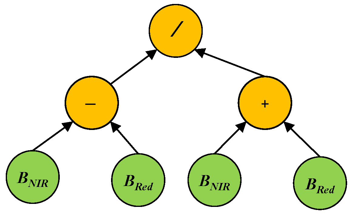
GP aims to automatically evolve computer programs (models or solutions) to solve a problem/task without requiring extensive domain knowledge [22]. Following the principles of Darwinian evolution and natural selection, GP can automatically evolve a population of programs to search for the best solution via several generations/iterations to solve specific problems. The programs/solutions of GP can be represented by different forms, such as trees, grammar, and linear. Among all these representations, tree-based GP is the most popular and widely used one. The trees are constructed by using functions or operators, such as +, −, ×, and protected /, to form the internal/root nodes, and using terminals, such as constants or variables/features, to form the leaf nodes. The functions are selected from a predefined function set, which often contains arithmetic and logic operators that can be used to solve this problem. The terminals are selected from a predefined terminal set, which often contains random constants and all the possible input variables/features of the problem. We take NDVI as an example to show the structure of a GP tree (Figure 1). In this example GP tree, the functions are /, +, and −, and the terminals are the NIR and Red bands. The GP tree can be formulated as , which is a feature constructed by using the NIR and Red bands.
The general process of GP starts by randomly initializing a population of trees (also called solutions, individuals, and programs) using a tree generation method [22]. Each tree is assigned a fitness value through fitness evaluation using a fitness function. The fitness value indicates how well the tree fits into the problem. GP searches for the best solution from the population via several generations, where the overall process is known as the evolutionary process. During the evolutionary process, better trees with higher fitness values have a large chance to survive and generate offspring for the next generation. These trees are selected by a selection method, and the offspring are generated from the selected trees (known as parents) using genetic operators. The commonly used genetic operators are crossover, mutation, and elitism of the subtree. A new population is generated using these operators for the next generation. The overall evolutionary process proceeds until it satisfies a termination criterion, and the best tree is returned. On a feature learning task, the best tree indicates the best feature set.
3. GP-Based Feature Learning for Crop Classification
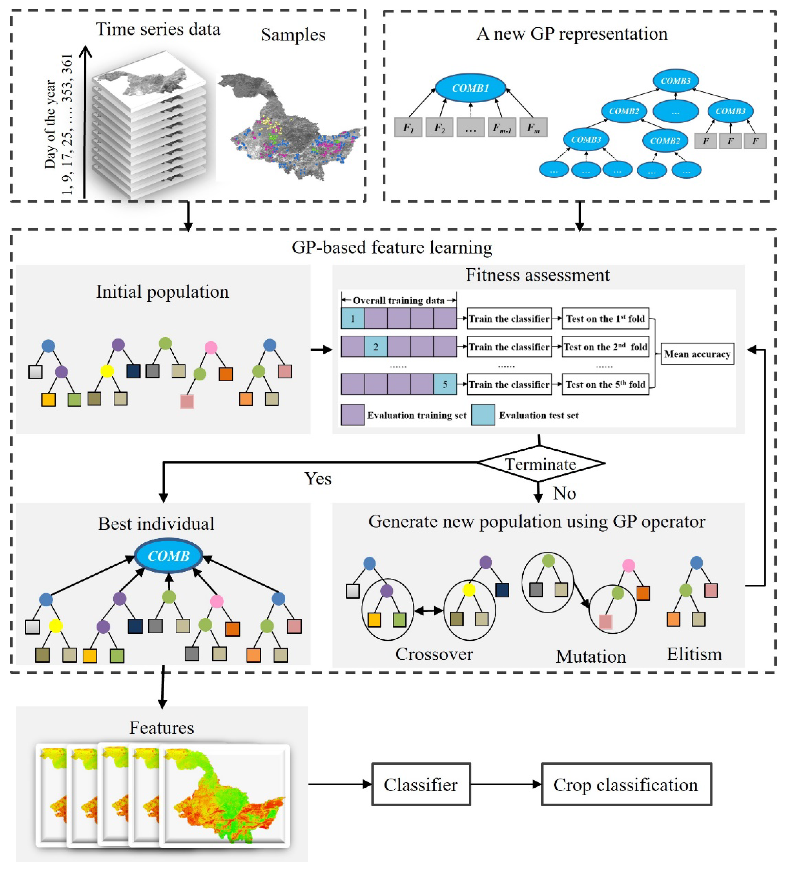
The overview of the whole GP approach for feature learning in crop classification is shown in Figure 2. We developed a new GP representation with a set of COMB functions, i.e., COMB1 as the root node to generate a fixed number of features, and COMB2 and COMB3 as the internal/root nodes to generate a dynamic number of features. The feature learning process of GP starts by randomly generating an initial population of trees based on the new representation, functions, and terminal sets. A new fitness function is designed to evaluate the goodness of each tree in the population with the training samples. At each generation, a new population is generated using the selection method and three common genetic operators, i.e., elitism, crossover, and mutation, to replace the current population. Then, the new population is evaluated using the fitness function, and evaluation processes are repeated until the maximum number of generations. Then the best GP tree is returned and applied to generate informative features for crop classification. The important parts of GP approach for high-level feature learning include the new GP representation, function and terminal sets, fitness function, and genetic operators, which are described in detail below.
3.1. The New Tree Representation of GP
Two representations of GP with COMB functions are developed to automatically learn/generate a predefined number or a dynamic number of features from the input data. The tree representation is based on strongly typed GP, where type constraints must be met when building new trees in the population initialization process and the genetic operations, i.e., crossover and mutation. The followings present how the GP trees are built using these different COMB functions in two ways.
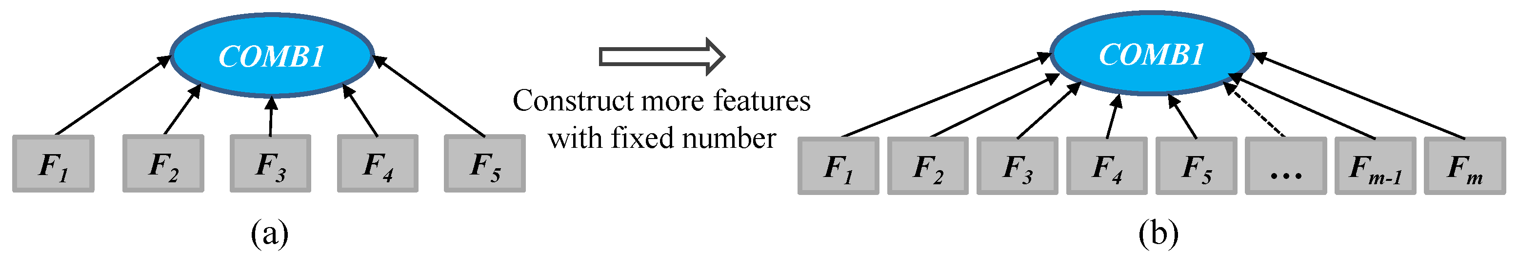
In the first tree representation, the function COMB1 is used as a root node to produce features with a fixed size. In other words, the root node of a GP tree has a predefined number of child nodes to produce features. An example tree with COMB1 that produces five different features is shown in Figure 3. This example program has five branches split from the root node COMB1. Each branch is a normal GP tree that can produce one feature using arithmetic operators. For example, the first feature F1 is , which indicates that the learned feature is a combination of the three bands. The five features are learned using different operators and the original bands.
The tree representation with function COMB1 is further extended by increasing the width of the tree to construct more high-level features with a fixed number (Figure 4). In this representation, we can define a number of learned features, and then the representation is extended to include more branches as each branch can produce a feature. For example, if m features are expected to be learned for crop classification, the GP representation can be changed to have m branches by designing a new root node COMB1. As shown in Figure 4b, the COMB1 function has m branches that produce m features. This new design of the COMB1 node allows GP to generate a predefined number of features for crop classification.
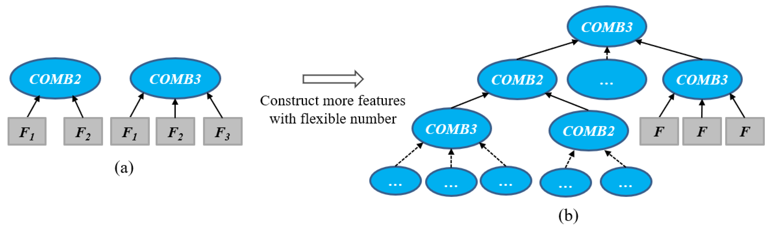
In the second tree representation, the COMB2 and COMB3 functions are developed as internal and root nodes to allow GP to learn a dynamic/flexible number of features by increasing the depth of the tree. The COMB2 and COMB3 functions accept two or three nodes as child nodes and can combine features from their child nodes. When the COMB2 or COMB3 function only appears at the root node, a GP tree can produce two or three features, respectively (as shown in Figure 5a). When the COMB2 and COMB3 functions appear at both internal and root nodes, a GP tree can concatenate the features from the internal nodes and has a deeper size to produce a large flexible number of features (as shown in Figure 5b). Compared with the first representation (Figure 4), the second representation does not need to predefine the number of features by automatically learning a dynamic number of features. The internal nodes and root nodes of COMB2 and COMB3 in GP trees determine the number of the features.
3.2. Function Set and Terminal Set
The function set includes the COMB functions (COMB1, COMB2, and COMB3), four arithmetic operators (, , , protected /), and a logic operator (IF) (Table 1). Except for the COMB functions, the other functions are commonly used for feature learning in the GP community. The COMB functions were specifically developed to allow the proposed approach to generate additional high-level features using a single tree. The four arithmetic functions each take two arguments as inputs and return one floating-point number. The division operation (/) is protected by returning one if the divisor is zero. The logic function IF returns one number by taking three arguments as inputs.
The terminal set includes original band values and random constants. The original bands are from the time series images for crop classification. Specifically, there are 217 band values for a pixel/example/instance as inputs of GP trees, where more details of them will be presented in Section 4.2. The random constants are random floating-point numbers sampled within the range [0.0, 1.0].
3.3. Fitness Function
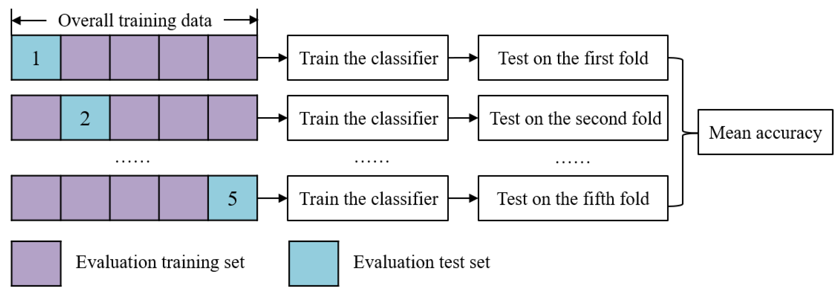
During the evolution of GP, the effectiveness of the features learned by GP is evaluated by using a fitness function. The fitness function is the classification accuracy obtained by an external classification algorithm (such as KNN, NB, DT, or SVM) with five-fold cross-validation using all samples in the training set.
In the fitness evaluation process, all samples with band values in the training set are transformed into features using a GP tree, and then the transformed training set is split into five folds. Four folds (evaluation training set) are used to train the classifier and the other one fold (evaluation test set) is used to evaluate the classifier and calculate the accuracy. This process repeats five times until each fold is used as the evaluation test set exactly once. The detailed process is shown in Figure 6. The test accuracy of each fold is defined in Equation (1), and the mean accuracy is calculated in Equation (2) as the fitness function.
where , , , and are the numbers of true positives, true negatives, false negatives, and false negatives of the corresponding (nth) fold, respectively. The acc and Fitness are in the range of [0, 1].
3.4. Genetic Operators
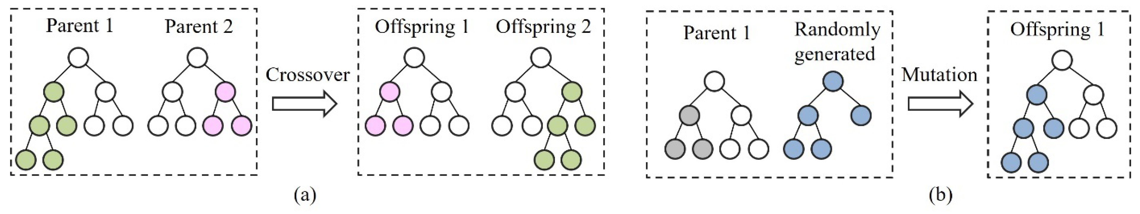
At each generation of GP, selection and genetic operators, including elitism, subtree crossover, and subtree mutation, are employed to create a new population to construct more promising features. The elitism operator copies several best trees with good fitness values from the current population to the new population. We apply tournament selection as the selection method to select trees with better fitness from the current population for crossover and mutation. The subtree crossover operator creates two new trees (offspring) by randomly selecting a branch of two trees (parents) and swapping the selected branches (Figure 7a). The subtree mutation operator creates a new tree (offspring) by randomly selecting one branch from a tree (parent) and replacing it with a new randomly generated branch (Figure 7b). In the GP approach with the COMB1 function, the genetic operators, i.e., crossover and mutation operators, do not change the root node since all GP methods use the same root node. In the GP approach with the COMB2 and COMB3 functions, the genetic operators work on the nodes with the same input and output types, i.e., meeting the constraints of the input and output types of nodes. The genetic operators not only maintain the goodness of the current population but can also search for promising spaces to produce the best features.
4. Experiment Design
4.1. Study Area
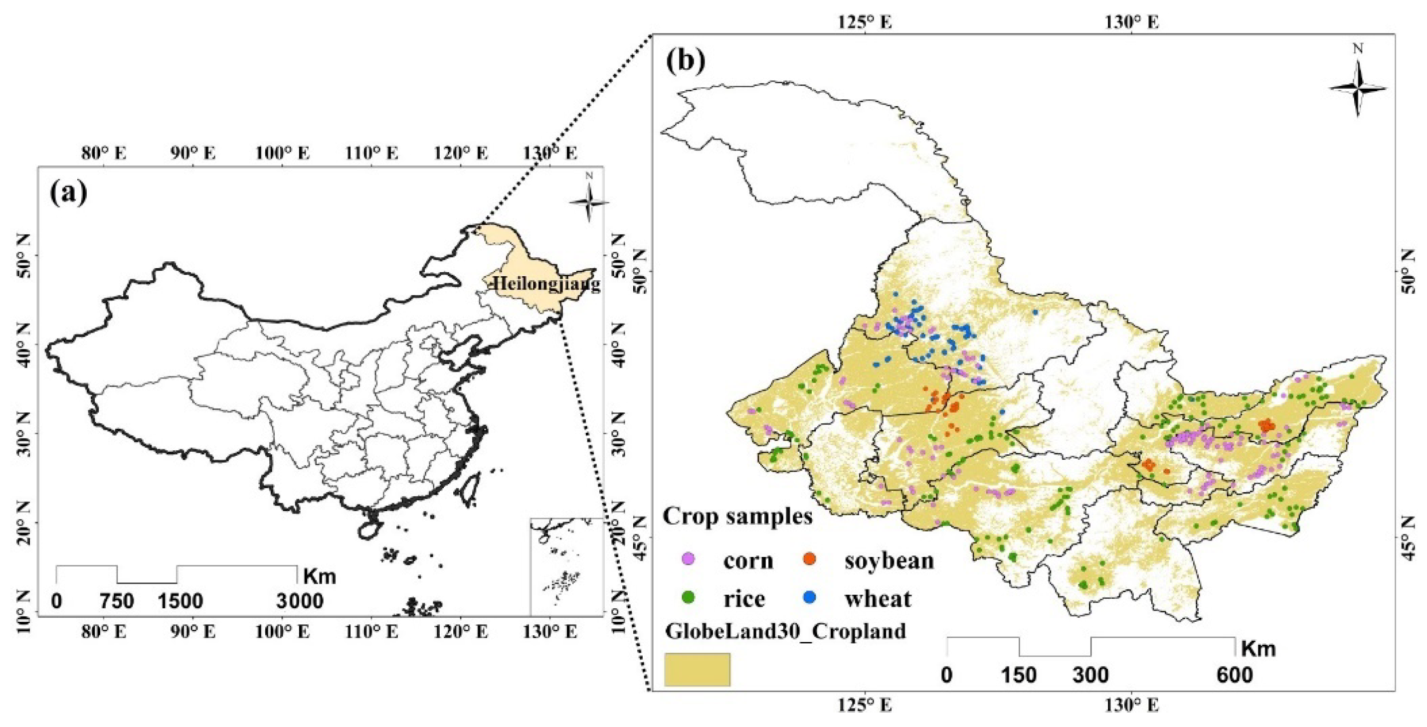
The study area was in Heilongjiang Province, located in northeastern China (Figure 8). Heilongjiang is the major agricultural region of China and has the largest grain production in the country. The cropland area in Heilongjiang Province is about 159,440 km2 according to the second national land survey of China [28]. Corn, soybean, rice, and wheat are the predominant crops. The study area has a humid continental climate, with a long bitter winter and a short warm summer. The annual average rainfall is 400 to 700 mm, concentrated heavily in the summer, and the annual average temperature is −4 °C to 4 °C, with 2200–2900 h of sunshine. As a result, Heilongjiang Province adopts a single cropping season system.
4.2. Data Collection and Preprocessing
We used MODIS Surface Reflectance Product (MOD09A1) of 8-day composites with a 500-m resolution, and each MOD09A1 pixel contained the best possible observation during 8 days (https://lpdaac.usgs.gov/products/mod09a1v006/, accessed on 1 August 2021). The input data of GP was the original seven bands of MOD09A1 with 8-day time series to learn high-level features for crop classification. The study area was covered by four MODIS tiles, i.e., h27v04, h26v04, h26v03, and h25v03. We selected the images from DOY (day of year) 65 to DOY 305 (31 composite periods) in 2011, spanning the critical period of the growing season. The data preprocessing included reprojection, mosaicking, and clipping. Finally, we obtained the time series images of MOD09A1 with the WGS84 projection covering the entire Heilongjiang Province. Because we focused on crop classification, we utilized the cropland distribution of GlobeLand30 to extract the cropland areas (Figure 8).
We utilized stratified random sampling to obtain the samples based on existing crop maps. Then the samples were identified with high-spatial-resolution images and field surveys. We obtained a total of 1131 crop samples, including rice, corn, soybean, and wheat. The training set included 411 samples (150 corn samples, 148 rice samples, 60 soybean samples, and 53 wheat samples), and the remaining 720 samples (300 corn samples, 300 rice samples, 70 soybean samples, and 50 wheat samples) were used for testing, which was consistent with our previous experiments [29].
4.3. Crop Classification Experiments and Parameter Settings
Firstly, the proposed GP approach with the new representations was evaluated by automatically learning fixed and flexible numbers of features from the time series data, respectively. We employed the new GP approach with the COMB1 function as the root node to learn a fixed number of features (Figure 4). The number of arguments/inputs in the COMB1 function was set as 5, 10, 15, 20, 25, and 30, enabling the proposed approach to learn 5, 10, 15, 20, 25, and 30 features, respectively. The GP approach with the COMB2 and COMB3 functions was used to learn a dynamic/flexible number of features (Figure 5). By conducting this group of experiments, we analyzed whether and how different numbers of features learned by GP affected crop classification performance.
Then, KNN, NB, DT, and SVM, were wrapped with the GP to analyze the influence of different classification algorithms on the crop classification. These four algorithms are representative classification algorithms that can build an instance-based classifier, a probability-based classifier, a tree-based classifier, and a linear classifier, respectively. The four classification algorithms were conducted by scikit-learn of the Python package [30]. In KNN, the number of neighbors was set to five. In SVM, a linear kernel was used since it provided better results than the other kernels and required fewer parameters. The penalty parameter value was one in SVM. The NB classifier is based on the Gaussian Naïve Bayes classification algorithm. For simplicity and easy reproduction, the parameter settings of these methods including MLP are default settings of the scikit-learn package [30]. In all of the above methods, all the 411 training samples are used for evolutionary learning and classifier training, and the classification/test accuracy is calculated using the 720 test samples.
The GP approach was implemented using the DEAP (Distributed Evolutionary Algorithm in Python) package with the parameter settings following the common settings in the GP community [17]. For every setting, i.e., each classification algorithm with a fixed or flexible number of features, GP runs independently 30 times because GP is a stochastic algorithm. The classifier with the highest test accuracy of the 30 runs was used as the final result of crop classification following the same setting in [26].
4.4. Comparison Experiments
The features with fixed number learned by GP were compared with the traditional features of VIs to investigate whether the features of GP can achieve better performance than the VI features. We first manually calculated five VIs (EVI, normalized difference tillage index (NDTI), land surface water index (LSWI), green vegetation index (VIgreen), and normalized difference senescent vegetation index (NDSVI)) for each composite period with a total of 155 VI features from the original spectrum channels. The minimum pairwise separability index (SImin) was used to calculate the minimum value separability of VIs and select the optimal features with fixed numbers (i.e., 5, 10, 15, 20, 25, and 30) for classification [29]. The classifiers KNN, NB, DT, and SVM were also used for crop classification based on the selected VI feature sets. Then the classification accuracies of the same test set were compared with that of GP.
The flexible number of features learned by GP were compared with MLP. We selected MLP to represent the popular deep learning method for classification due to the limitation of training sample size. In these comparisons, different numbers of training samples were employed for GP and MLP training to obtain flexible number of features and then used for the classification. In the experiments, the subset was randomly selected from the original training set using a proportion, i.e., 40%, 50%, 60%, 70%, 80%, 90%, and 100%, and the subset was used for feature learning and classifier training. The test set was kept the same and the classification accuracies of these methods were calculated on the test set for comparisons. We used the default settings of the MLP in the scikit-learn package for simplification. The activation function was a rectified linear unit function (ReLU), and the optimizer was Adam. The maximum number of iterations was 200. The MLP method takes the raw pixels as inputs and transforms the raw inputs into features to perform classification. Note that MLP may not be the state-of-the-art NN-based method for this problem. Since there is no NN-based method for this problem and other NN-based methods such as CNNs and Transformers have a large number hyperparameters, which are difficult to set, only the simple NN—MLP was used for comparisons.
5. Results and Analysis
5.1. Crop Classification Results
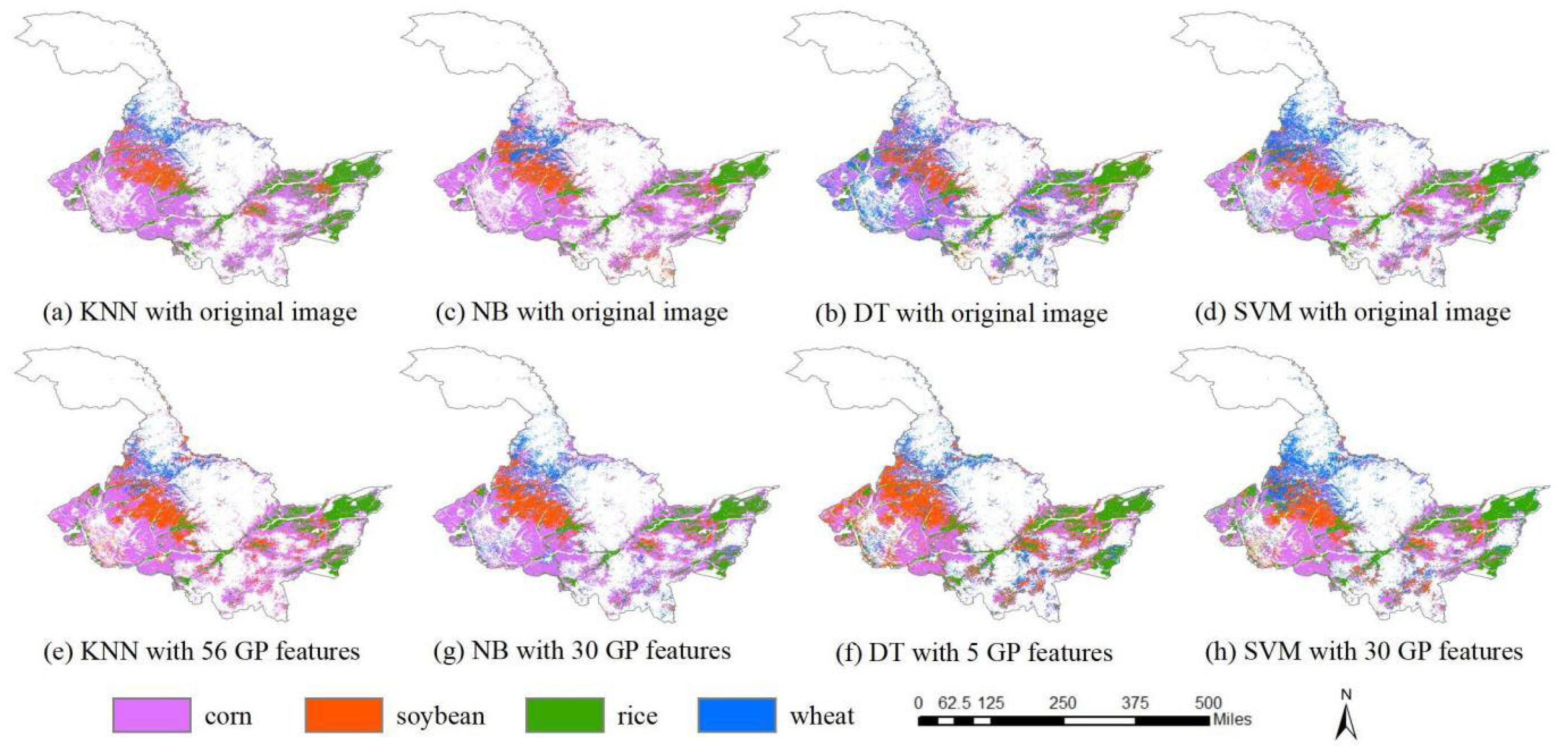
The classification results with the original time series images by using KNN, NB, DT, and SVM are shown in Figure 9a–d, and the classification accuracies are shown in Table 2. By comparison, the classification results with the highest accuracies by using features of GP for each classifier (values in bold in Table 2) are shown in Figure 9e–h. For KNN, the highest accuracy was 97.78% with the flexible number of features. The highest accuracies of NB, DT, and SVM were 97.08%, 96.11%, and 97.78%, and the fixed numbers of features used were 30, 5, and 30, respectively (Table 2). The classification results show that the proposed GP method markedly improved the classification accuracy compared with the classification using original images. The classification accuracies of KNN were improved greatly using the features learned by GP. The KNN classification accuracy by using the original image was 89.72%, while the accuracies by using the GP learned features were all over 96.11%. The classification accuracy of NB using the original image was 92.50%, which is much less than any of the accuracies obtained using the features learned by GP. The classification accuracy of DT using the original image was 94.03%, and the accuracies were improved by using GP-based feature learning. The classification accuracy of SVM by using the original image was 97.22%, while the accuracies using features learned by GP were higher than or equal to that of the original data, except for feature number five.
With the features learned by GP, the classification accuracies of KNN and NB were improved more than those of DT and SVM. KNN with GP features achieved the largest increase of 8.06% in classification accuracy (from 89.72% to 97.78%), and NB obtained the larger increase of 5.03% in classification accuracy by using GP features (from 92.05% to 97.08%). In contrast, DT with GP features improved the accuracy from 94.03% to 96.11% by using features learned by GP, and SVM increased the classification accuracy from 97.22% with raw images to 97.78%, which was the smallest accuracy increase. Because DT and SVM select features or optimize weights for features when training the classifiers, the accuracy improvements of DT and SVM were small. In contrast, KNN and NB, which are weak classifiers, treat each feature equally. The accuracy improvements of KNN and NB demonstrate the effectiveness of the proposed GP method for crop classification.
The number of features has little effect on classification accuracy in the GP method. Most studies on feature selection found that the classification accuracies initially increase with more features and then decrease after the accuracies reach a peak, which is the well-known Hughes effect [31]. In contrast, fewer features learned by GP can achieve better accuracy, and the effect of the number of features on the classification accuracy is not obvious. Specifically, when the feature number was fixed, KNN obtained the highest accuracy of 97.36% with 10 features and the lowest accuracy of 96.11% with 25 features. NB reached the highest accuracy with 30 features, while 5 and 25 features had the same accuracies. Therefore, the accuracies of NB were not increased when the feature sizes were increased from 5 to 30. Similarly, there were no remarkable relationships between classification accuracies and feature numbers for DT and SVM.
The performance of GP learning a flexible number is not always better than that of learning a fixed number for crop classification. The best classification accuracy of KNN was 97.78% with a flexible feature number of 56 (Table 2), which is higher than the accuracies with the fixed number of features. Yet, the accuracies with a flexible number of features for other classifiers were not higher than those with a fixed number of features. The accuracies of NB, DT, and SVM were 96.67%, 95.14%, and 97.22% with a flexible number of features, which are lower than some accuracies of features with a fixed number. Therefore, using GP to learn a flexible number of features might not always increase the classification accuracy compared with fixed number of features. This is because when the number of the feature is flexible the search space of GP is larger than when learning a fixed number of features. GP needs a larger population and a longer time to search for the best solutions from the larger search space. This aspect can be further investigated in future research.
5.2. Feature Visualization and Analysis
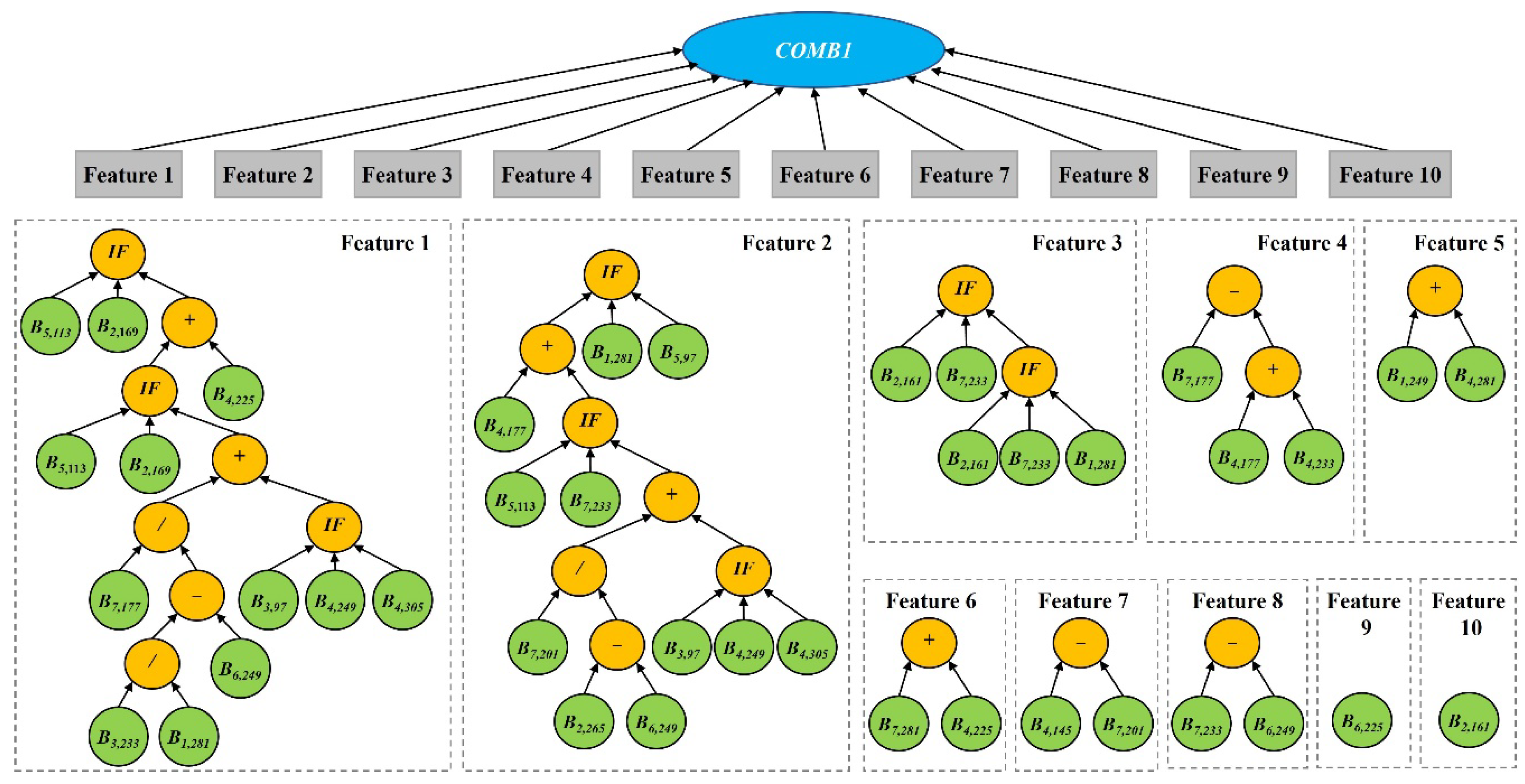
We took 10 features as an example to visualize the features learned by GP with KNN. The classification accuracy of KNN with these 10 learned features was 97.36% (Table 2). We used a single tree of the new representation to visualize the 10 features (Figure 10). The root node of COMB1 has 10 branches, and each branch is a learned feature constructed by different functions and bands. The terminals are the input time series MODIS bands, and the functions are mainly arithmetic functions (, , , and protected /) and the logic function (IF) (Table 1). Features 1 to 8 used various bands and functions to construct features and represent high-level information of the original bands. GP can not only be used to construct the new high-level features automatically but also as a feature selection method simultaneously. Feature 9 is B6, 225, which is the SWIR band on DOY 225. Feature 10 is B2,161, which is the NIR band on DOY 161. These two bands are sensitive to vegetation water and growth.
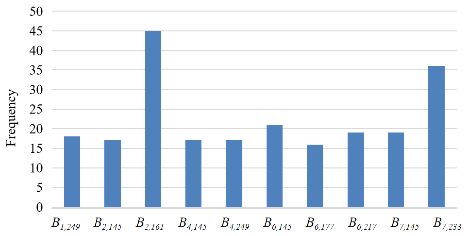
We analyzed the usage frequency of the original bands in the GP method learning fixed and flexible numbers of features. The top 10 bands with high usage frequency were Bands 2, 6, and 7 (Figure 11). Band 2 is NIR with a wavelength from 841 to 876 nm, which is a strong reflection band for vegetation. Band 2 can reveal chlorophyll content in crops and is widely used for crop identification [15,32]. Bands 6 and 7 are SWIR bands, and the vegetation reflectance decreases in these two bands because incoming radiation is strongly absorbed by water. The SWIR bands can be used to retrieve information on vegetation water content over a crop-growing period. Most vegetation indices combine information contained in NIR and SWIR, such as NDVI, EVI, and NDTI.
The top 10 bands were mainly from DOYs 145-177 and 217-249, optimal window periods for crop identification. DOYs 145-177 (from late May to late June) are the rice transplanting and green-up periods in Heilongjiang [29]. This period can be easily used to identify rice because paddy fields are inundated and show higher water levels than other fields. Wheat seedlings range from three leaves to the jointing stage and have a vegetation coverage that is higher than that of corn and soybean. DOYs 217-249 are in the optimal window period of maturity for crop identification. In this period, wheat is harvested earliest, and, after harvest, its soil moisture and vegetation cover are significantly lower than those of other crops. Additionally, the leaves of soybean become yellow and dry during the period of seed filling, which is different from other crops. The analysis further reveals that GP can automatically find useful patterns, select important features from the original features, and construct useful high-level features for effective crop classification without relying on extensive domain knowledge and experience.
5.3. Comparisons with VIs
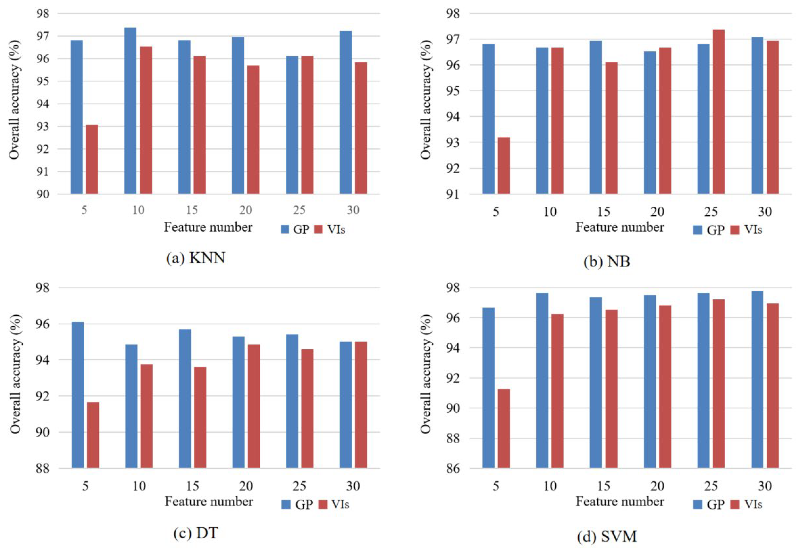
We selected 5, 10, 15, 20, 25, and 30 features from 155 original VIs by using SImin, and the classification accuracies of KNN, NB, DT, and SVM were compared with those of features learned by GP (Figure 12). The accuracies of the four classifiers with features of GP were generally higher than those derived from VIs. Especially for the five features, the accuracies of the four classifiers using GP features were more than 96.10%, whereas the accuracies using VIs were less than 93.50%. The accuracies of VIs were steadily improved with the increase in the number of features, and the accuracy gaps between GP and VIs were gradually narrowed. The accuracies of NB using features learned by GP were slightly lower than those using VI features when the feature numbers were 20 and 25. For the other classifiers, GP features showed remarkable advantages compared with VIs.
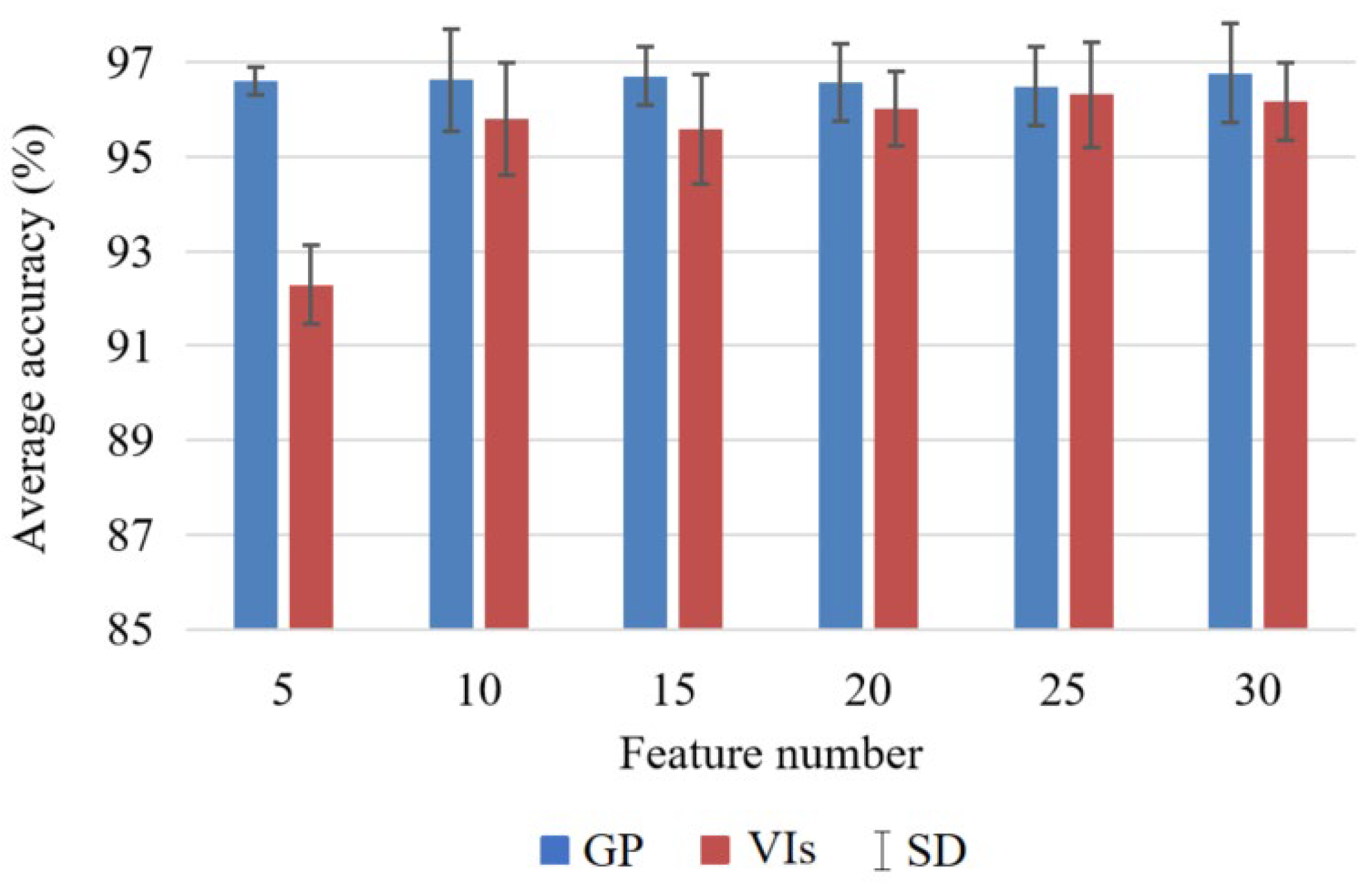
We calculated the average accuracies and standard deviations (SDs) using different classifiers with each feature set from GP and VIs (Figure 13). The average accuracies of the GP-based features were higher than those obtained from VIs, indicating the better performance of GP. The average accuracies of features learned by GP ranged from 96.50% to 96.77%, with minor differences. In contrast, the average accuracies of VIs increased and SDs decreased with more features. The lowest average accuracy of VIs was 92.29% when using 5 features, whereas the highest accuracy was 96.32% when using 25 features. From the comparisons, it is clear that the number of GP features has little effect on classification accuracy, while it is very crucial for the VIs. Therefore, the GP method is more robust and stable than the VIs in terms of the feature number.
The SDs describe the accuracy differences of the four classifiers when using the same number of features. The SDs of GP ranged from 0.29 to 1.08, while the SDs of VIs were from 0.82 to 1.19. Taking five features as an example, the SDs of GP and VIs were 0.29 and 0.85, respectively, which indicated the classification differences of the GP method with the four classifiers (i.e., KNN, NB, DT, and SVM) were less than with the VI features. Overall, the SDs of GP were always lower than those of VIs. The results indicate that for the same number of features, the accuracy differences of GP are lower with different classifiers for crop classification. Therefore, it is reasonable to assume that GP is more stable than VIs for various classifiers.
5.4. Comparisons with MLP
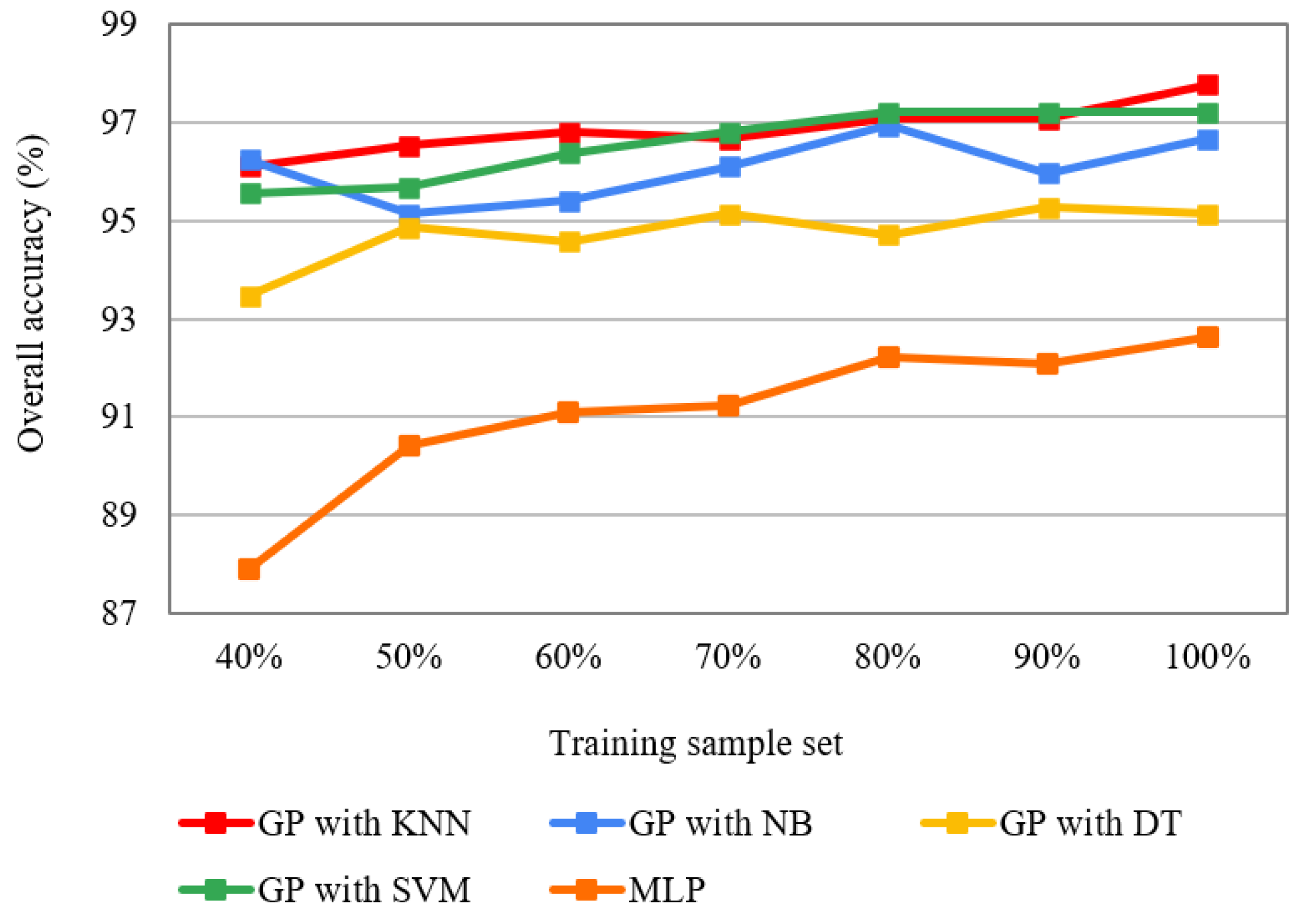
The overall accuracies of GP with the flexible number of features wrapped with the four classifiers (i.e., KNN, NB, DT, and SVM) by using 40%, 50%, 60%, 70%, 80%, 90%, and 100% training sets were assessed and compared with those of MLP (Figure 14). Firstly, the higher accuracies with various training sets indicate that GP performed better for feature learning compared with the MLP. Second, GP can achieve excellent accuracy even with a small training subset. For example, the overall accuracies of GP with KNN and NB were 96.11% and 96.25% with 40% training subsets. Moreover, the number of training samples has less influence on GP than the MLP, and the accuracy of GP does not always increase as the sample number increases. For example, the GP with NB had the lowest accuracy using 50% training samples and the highest accuracy with 80% of the training subset. Similarly, the accuracies of GP with DT slightly fluctuated as the sample number increased. In comparison with GP, the higher the number of training samples, the higher the overall accuracies of the MLP. Additionally, the accuracy fluctuation of the MLP was higher than that of GP. The accuracy of MLP is increased from 87.92% (40% training samples) to 92.64% (100% training samples), while that of GP with KNN ranged from 96.11% to 97.78%.
6. Discussion
Automatic feature extraction is still challenging for crop classification because the manual methods are tedious, time-consuming, and subjective. GP is a very powerful and flexible method to automatically evolve mathematical models from a set of terminals and operators without extensive domain knowledge. We introduced a new GP method to automatically learn high-level, effective features based on time series images. We developed new representations for GP by using a set of COMB functions to automatically produce fixed and flexible numbers of high-level features from the time series data. The COMB1 function was developed to produce a predefined number of features by extending the width of the GP tree, while the COMB2 and COMB3 functions were proposed to produce a flexible number of features by extending the GP tree depth. The proposed GP method can automatically select valuable bands with typical spectral and temporal characteristics from the original data and simultaneously construct high-level features from the selected features using predefined operators or functions (Figure 10).
The features learned by GP significantly improved the classification accuracy for two reasons. The first one is that GP creates new features from the original features, and automatically transforms the original representation space into a new one that better represents the spatial and temporal characteristics of crops. The process of feature learning combines features selected from the original features and then creates new high-level features for classification. The second reason is that GP employs the fitness function wrapped with a classifier to assess the effectiveness of the learned features in the evolutionary process.
GP is more robust and stable with various classifiers and different numbers of features compared with VIs. The average accuracy differences of the four classifiers are small using features learned by GP, while they are large when using VIs. The feature number of GP has little effect on the classification performance since classification accuracy is high even with only five GP-based features. By contrast, VIs usually require a large number of features to reach the highest classification accuracy. Additionally, GP can achieve excellent accuracy even with a small training subset. The overall accuracy of MLP increases with more training samples, while GP is more stable with various training sets. The number of training samples has less influence on the classification accuracy of GP than that of MLP.
The features learned by GP are easier to understand and interpret because of their origin and formation compared with other feature learning methods such as deep learning. In the experiments, GP first identified the original bands with typical spectral and temporal characteristics for feature learning. Bands with high usage frequencies for GP were NIR and SWIR bands, which are also widely used to construct vegetation indices (such as EVI and NDVI). Meanwhile, most bands were selected during DOYs 145-177 and 217-249, which are DOYs in the middle of the crop growing seasons and represent optimal window periods for crop identification in Heilongjiang Province. Based on the selected bands, GP constructed new high-level features by the tree representation using a series of functions and operators (Table 1). Deep learning models (such as CNNs and other neural networks) can achieve high classification accuracy in several cases but are considered black boxes because they learn arcane features with poor interpretability. By comparison, GP has good interpretability and can explain how and why the features are obtained.
GP is one of the most versatile artificial intelligence methods but is still largely underused in remote sensing. Our study demonstrated the outstanding performance of GP for feature-learning based on MODIS time series images, suggesting that it is worthwhile to explore its potential applications in remote sensing. The GP for feature learning with dynamic/flexible number is more promising because predefining the number of features is not necessary. However, this method may not always achieve the best accuracy, because the search space of GP is much larger than with learning a fixed number of features, and the model suffers from local optima. How to automatically decide the optimal number of constructed features with high classification accuracy is still an open issue and needs further research. In practice, GP can also be used for classifier construction with its flexible representation and distinctive features [33]. GP will be investigated in future work to explore additional applications using higher spatial and temporal images, such as tree-based GP for image classification, feature transfer learning, and change detection.
7. Conclusions
We developed a novel GP approach to learn high-level features for crop classification using time series images to address the inefficiencies of manual feature extraction in this study. We proposed a new GP representation with a single tree to flexibly learn multiple high-level features. GP with this representation produces high-level features by increasing the widths or depths of the trees based on a set of COMB functions. We employed four classifiers (KNN, NB, DT, and SVM) for crop classification by using the features learned by GP, and the accuracies were significantly improved. Compared with the traditional VIs features, GP demonstrated better performance and robustness for various classifiers and feature numbers. Additionally, we found that the number of training samples influenced GP less compared with MLP and that GP could produce excellent accuracy even with a small training subset.
This was the first time that GP was utilized to learn multiple features for crop classification by using time series images. The new GP approach automatically selected discriminable low-level features from the original band images and learned additional high-level features without domain knowledge. This study showed the advantages of GP in feature learning, i.e., flexible representation and high interpretability. These promising results demonstrated the potential of GP in remote sensing, which will be further explored by applying it to more applications with higher resolution data in the future. In addition, it is possible to investigate different experiment designs such as using the validation set to further improve the performance of the GP approach on real-world applications.
Author Contributions
M.L., Y.B., B.X. and M.Z. proposed the GP method for crop classification and designed the experiments; M.L., Q.H., P.Y., Y.W. and W.W. prepared the remote sensing data and conducted the experiments of SImin; M.L. and Y.B. developed the model code of GP and conducted the experiments of GP; M.L. prepared the manuscript and wrote the final paper with contributions from all the co-authors. All authors have read and agreed to the published version of the manuscript.
Funding
This research was funded by the National Natural Science Foundation of China (41921001, 42071419), the Fundamental Research Funds for Central Non-profit Scientific Institution (1610132020016), the Agricultural Science and Technology Innovation Program (ASTIP No. CAAS-ZDRW202201), the National Key Research and Development Program of China (2019YFA0607400), and Project of Special Investigation on Basic Resources of Science and Technology (2019FY202501).
Data Availability Statement
The MODIS Terra MOD09A1 product used in this study is openly available from https://lpdaac.usgs.gov/products/mod09a1v006/ (accessed on 28 June 2022). The code is available from the corresponding author upon reasonable request.
Conflicts of Interest
The authors declare no conflict of interest.
References
- Gao, L.; Bryan, B.A. Finding pathways to national-scale land-sector sustainability. Nature 2017, 544, 217–222. [Google Scholar] [CrossRef] [PubMed]
- Cui, Z.; Zhang, H.; Chen, X.; Zhang, C.; Ma, W.; Huang, C.; Zhang, W.; Mi, G.; Miao, Y.; Li, X.; et al. Pursuing sustainable productivity with millions of smallholder farmers. Nature 2018, 555, 363–366. [Google Scholar] [CrossRef] [PubMed]
- Renard, D.; Tilman, D. National food production stabilized by crop diversity. Nature 2019, 571, 257–260. [Google Scholar] [CrossRef] [PubMed]
- Veloso, A.; Mermoz, S.; Bouvet, A.; Le Toan, T.; Planells, M.; Dejoux, J.-F.; Ceschia, E. Understanding the temporal behavior of crops using Sentinel-1 and Sentinel-2-like data for agricultural applications. Remote Sens. Environ. 2017, 199, 415–426. [Google Scholar] [CrossRef]
- Johnson, D.M. Using the Landsat archive to map crop cover history across the United States. Remote Sens. Environ. 2019, 232, 111286. [Google Scholar] [CrossRef]
- Zhong, L.; Hu, L.; Zhou, H. Deep learning based multi-temporal crop classification. Remote Sens. Environ. 2019, 221, 430–443. [Google Scholar] [CrossRef]
- Pôças, I.; Calera, A.; Campos, I.; Cunha, M. Remote sensing for estimating and mapping single and basal crop coefficientes: A review on spectral vegetation indices approaches. Agric. Water Manag. 2020, 233, 106081. [Google Scholar] [CrossRef]
- Xue, J.; Su, B. Significant Remote Sensing Vegetation Indices: A Review of Developments and Applications. J. Sens. 2017, 2017, 1353691. [Google Scholar] [CrossRef]
- Huete, A.; Didan, K.; Miura, T.; Rodriguez, E.P.; Gao, X.; Ferreira, L.G. Overview of the radiometric and biophysical performance of the MODIS vegetation indices. Remote Sens. Environ. 2002, 83, 195–213. [Google Scholar] [CrossRef]
- Zhang, G.; Xiao, X.; Biradar, C.M.; Dong, J.; Qin, Y.; Menarguez, M.A.; Zhou, Y.; Zhang, Y.; Jin, C.; Wang, J.; et al. Spatiotemporal patterns of paddy rice croplands in China and India from 2000 to 2015. Sci. Total Environ. 2017, 579, 82–92. [Google Scholar] [CrossRef]
- Zhang, G.; Xiao, X.; Dong, J.; Xin, F.; Zhang, Y.; Qin, Y.; Doughty, R.B.; Moore, B. Fingerprint of rice paddies in spatial–temporal dynamics of atmospheric methane concentration in monsoon Asia. Nat. Commun. 2020, 11, 554. [Google Scholar] [CrossRef]
- Chang, J.; Hansen, M.C.; Pittman, K.; Carroll, M.; DiMiceli, C. Corn and Soybean Mapping in the United States Using MODIS Time-Series Data Sets. Agron. J. 2007, 99, 1654–1664. [Google Scholar] [CrossRef]
- Song, X.-P.; Potapov, P.V.; Krylov, A.; King, L.; Di Bella, C.M.; Hudson, A.; Khan, A.; Adusei, B.; Stehman, S.V.; Hansen, M.C. National-scale soybean mapping and area estimation in the United States using medium resolution satellite imagery and field survey. Remote Sens. Environ. 2017, 190, 383–395. [Google Scholar] [CrossRef]
- Bargiel, D. A new method for crop classification combining time series of radar images and crop phenology information. Remote Sens. Environ. 2017, 198, 369–383. [Google Scholar] [CrossRef]
- Wang, S.; Azzari, G.; Lobell, D.B. Crop type mapping without field-level labels: Random forest transfer and unsupervised clustering techniques. Remote Sens. Environ. 2019, 222, 303–317. [Google Scholar] [CrossRef]
- Zhong, L.; Gong, P.; Biging, G.S. Efficient corn and soybean mapping with temporal extendability: A multi-year experiment using Landsat imagery. Remote Sens. Environ. 2014, 140, 1–13. [Google Scholar] [CrossRef]
- Bi, Y.; Xue, B.; Zhang, M. An Effective Feature Learning Approach Using Genetic Programming With Image Descriptors for Image Classification [Research Frontier]. IEEE Comput. Intell. Mag. 2020, 15, 65–77. [Google Scholar] [CrossRef]
- Zhang, L.; Zhang, L.; Du, B. Deep Learning for Remote Sensing Data: A Technical Tutorial on the State of the Art. IEEE Geosci. Remote Sens. Mag. 2016, 4, 22–40. [Google Scholar] [CrossRef]
- Zhang, C.; Sargent, I.; Pan, X.; Li, H.; Gardiner, A.; Hare, J.; Atkinson, P.M. Joint Deep Learning for land cover and land use classification. Remote Sens. Environ. 2019, 221, 173–187. [Google Scholar] [CrossRef]
- Eiben, A.E.; Smith, J. From evolutionary computation to the evolution of things. Nature 2015, 521, 476–482. [Google Scholar] [CrossRef]
- Koza, J.R. Genetic Programming: On the Programming of Computers by Means of Natural Selection; MIT Press: Cambridge, MA, USA, 1992. [Google Scholar]
- Tran, B.; Xue, B.; Zhang, M. Genetic programming for multiple-feature construction on high-dimensional classification. Pattern Recognit. 2019, 93, 404–417. [Google Scholar] [CrossRef]
- Ain, Q.U.; Al-Sahaf, H.; Xue, B.; Zhang, M. Generating Knowledge-Guided Discriminative Features Using Genetic Programming for Melanoma Detection. IEEE Trans. Emerg. Top. Comput. Intell. 2021, 5, 554–569. [Google Scholar] [CrossRef]
- Liang, Y.; Zhang, M.; Browne, W.N. Figure-ground image segmentation using feature-based multi-objective genetic programming techniques. Neural Comput. Appl. 2019, 31, 3075–3094. [Google Scholar] [CrossRef]
- Puente, C.; Olague, G.; Trabucchi, M.; Arjona-Villicaña, P.D.; Soubervielle-Montalvo, C. Synthesis of Vegetation Indices Using Genetic Programming for Soil Erosion Estimation. Remote Sens. 2019, 11, 156. [Google Scholar] [CrossRef]
- Cabral, A.I.R.; Silva, S.; Silva, P.C.; Vanneschi, L.; Vasconcelos, M.J. Burned area estimations derived from Landsat ETM+ and OLI data: Comparing Genetic Programming with Maximum Likelihood and Classification and Regression Trees. ISPRS J. Photogramm. Remote Sens. 2018, 142, 94–105. [Google Scholar] [CrossRef]
- Batista, J.E.; Cabral, A.I.; Vasconcelos, M.J.; Vanneschi, L.; Silva, S. Improving Land Cover Classification Using Genetic Programming for Feature Construction. Remote Sens. 2021, 13, 1623. [Google Scholar] [CrossRef]
- Tan, Y.; He, J.; Yue, W.; Zhang, L.; Wang, Q.R. Spatial pattern change of the cultivated land before and after the second national land survey in China. J. Nat. Resour. 2017, 32, 186–197. [Google Scholar] [CrossRef]
- Hu, Q.; Wu, W.; Song, Q.; Yu, Q.; Lu, M.; Yang, P.; Tang, H.; Long, Y. Extending the Pairwise Separability Index for Multicrop Identification Using Time-Series MODIS Images. IEEE Trans. Geosci. Remote Sens. 2016, 54, 6349–6361. [Google Scholar] [CrossRef]
- Pedregosa, F.; Varoquaux, G.; Gramfort, A.; Michel, V.; Thirion, B.; Grisel, O.; Blondel, M.; Prettenhofer, P.; Weiss, R.; Dubourg, V. Scikit-learn: Machine learning in Python. J. Mach. Learn. Res. 2011, 12, 2825–2830. [Google Scholar]
- Löw, F.; Michel, U.; Dech, S.; Conrad, C. Impact of feature selection on the accuracy and spatial uncertainty of per-field crop classification using Support Vector Machines. ISPRS J. Photogramm. Remote Sens. 2013, 85, 102–119. [Google Scholar] [CrossRef]
- Gitelson, A.A.; Viña, A.; Ciganda, V.; Rundquist, D.C.; Arkebauer, T.J. Remote estimation of canopy chlorophyll content in crops. Geophys. Res. Lett. 2005, 32, L08403. [Google Scholar] [CrossRef]
- Espejo, P.G.; Ventura, S.; Herrera, F. A Survey on the Application of Genetic Programming to Classification. IEEE Trans. Syst. Man Cybern. Part C (Appl. Rev.) 2010, 40, 121–144. [Google Scholar] [CrossRef]
Figure 1.
An example GP tree for NDVI.

Figure 2.
The workflow of GP for feature learning in crop classification.

Figure 3.
An example tree of the proposed GP method with the COMB1 function. This tree can produce five features, and each feature is constructed by using arithmetic operators and input bands (terminals).
Figure 3.
An example tree of the proposed GP method with the COMB1 function. This tree can produce five features, and each feature is constructed by using arithmetic operators and input bands (terminals).

Figure 4.
The new GP tree representation with COMB1 as a root node produces a predefined number of features by extending the width of the tree: using COMB1 to produce five features (a); and using COMB1 to produce m features (b). Fi denotes a subtree that produces a feature using functions (e.g., arithmetic operators) and terminals.

Figure 5.
The new representation with the COMB2 and COMB3 functions produces a flexible/dynamic number of features by extending the depth of the tree. COMB2 and COMB3 are only used as the root node to produce two and three features (a); while they are used as the root and internal nodes to produce more features (b). Fi denotes a subtree that produces a feature using functions (e.g., arithmetic operators) and terminals.

Figure 6.
Illustration of the five-fold cross-validation with a classification algorithm.

Figure 7.
Schematic of crossover (a); and mutation operations (b).

Figure 8.
The study area location (a) and crop samples (b).

Figure 9.
Classification results of KNN, NB, DT, and SVM by using original images (a–d); and GP learned features with the highest accuracies (e–h).
Figure 9.
Classification results of KNN, NB, DT, and SVM by using original images (a–d); and GP learned features with the highest accuracies (e–h).

Figure 10.
Example of 10 features learned by GP.

Figure 11.
The frequency of the top 10 bands used in the GP methods learning the fixed and flexible numbers of features.
Figure 11.
The frequency of the top 10 bands used in the GP methods learning the fixed and flexible numbers of features.

Figure 12.
Comparisons of classification accuracies of (a) KNN, (b) NB, (c) DT, and (d) SVM using features learned by GP and selected from VIs.
Figure 12.
Comparisons of classification accuracies of (a) KNN, (b) NB, (c) DT, and (d) SVM using features learned by GP and selected from VIs.

Figure 13.
The average accuracies and SDs of GP and VIs using different classifiers and feature numbers.
Figure 13.
The average accuracies and SDs of GP and VIs using different classifiers and feature numbers.

Figure 14.
The overall accuracies of the GP wrapped four classifiers (i.e., KNN, NB, DT and SVM), and MLP for various training subsets.
Figure 14.
The overall accuracies of the GP wrapped four classifiers (i.e., KNN, NB, DT and SVM), and MLP for various training subsets.


Table 1.
The function set of the proposed approach.
| Function | Type | No. Arguments | Descriptions |
|---|---|---|---|
| COMB1 | Root | m (Predefined) | Concatenate multiple inputs into a feature vector |
| COMB2 | Root/Internal | Two | Concatenate two inputs into a feature vector |
| COMB3 | Root/Internal | Three | Concatenate three inputs into a feature vector |
| Add (+) | Internal | Two | Add two arguments |
| Sub (−) | Internal | Two | Subtract two arguments |
| Mul (×) | Internal | Two | Multiply two arguments |
| ProD (/) | Internal | Two | Protected division. Divide the second argument using the first argument. Return one if the divisor is zero. |
| IF | Internal | Three | If the first argument is greater than 0, the second argument is returned. Otherwise, the third argument is returned. |
Table 2.
Classification accuracies of KNN, NB, DT, and SVM using original image and different numbers of features learned by GP.
Table 2.
Classification accuracies of KNN, NB, DT, and SVM using original image and different numbers of features learned by GP.
| KNN (%) | NB (%) | DT (%) | SVM (%) | ||
|---|---|---|---|---|---|
| Original image | 89.72 | 92.50 | 94.03 | 97.22 | |
| GP for fixed number of features | 5 | 96.81↑ | 96.81↑ | 96.11↑ | 96.67↓ |
| 10 | 97.36↑ | 96.67↑ | 94.86↑ | 97.64↑ | |
| 15 | 96.81↑ | 96.94↑ | 95.69↑ | 97.36↑ | |
| 20 | 96.94↑ | 96.53↑ | 95.28↑ | 97.50↑ | |
| 25 | 96.11↑ | 96.81↑ | 95.42↑ | 97.64↑ | |
| 30 | 97.22↑ | 97.08↑ | 95.00 ↑ | 97.78↑ | |
| GP for flexible number of features | 97.78↑ (56) | 96.67↑ (23) | 95.14↑ (32) | 97.22 = (65) |
Note: Numbers in italic in the last row indicate the number of features automatically learned by GP when this number was flexible. Symbols “↑”, “↓”, and “=” indicate that the accuracies are higher than, lower than, and equal to those of the original image (band values).
Publisher’s Note: MDPI stays neutral with regard to jurisdictional claims in published maps and institutional affiliations. |
© 2022 by the authors. Licensee MDPI, Basel, Switzerland. This article is an open access article distributed under the terms and conditions of the Creative Commons Attribution (CC BY) license (https://creativecommons.org/licenses/by/4.0/).
Share and Cite
MDPI and ACS Style
Lu, M.; Bi, Y.; Xue, B.; Hu, Q.; Zhang, M.; Wei, Y.; Yang, P.; Wu, W. Genetic Programming for High-Level Feature Learning in Crop Classification. Remote Sens. 2022, 14, 3982. https://doi.org/10.3390/rs14163982
AMA Style
Lu M, Bi Y, Xue B, Hu Q, Zhang M, Wei Y, Yang P, Wu W. Genetic Programming for High-Level Feature Learning in Crop Classification. Remote Sensing. 2022; 14(16):3982. https://doi.org/10.3390/rs14163982
Chicago/Turabian StyleLu, Miao, Ying Bi, Bing Xue, Qiong Hu, Mengjie Zhang, Yanbing Wei, Peng Yang, and Wenbin Wu. 2022. "Genetic Programming for High-Level Feature Learning in Crop Classification" Remote Sensing 14, no. 16: 3982. https://doi.org/10.3390/rs14163982
Note that from the first issue of 2016, this journal uses article numbers instead of page numbers. See further details here.