Estimating Water pH Using Cloud-Based Landsat Images for a New Classification of the Nhecolândia Lakes (Brazilian Pantanal)

 , , ,
, , ,
Abstract
: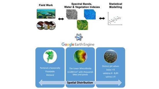
1. Introduction
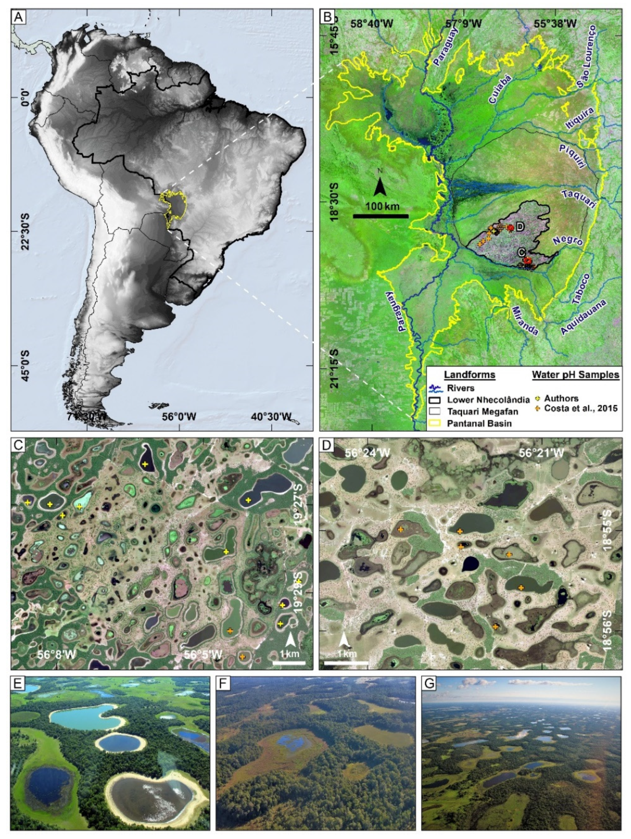
2. Regional Settings
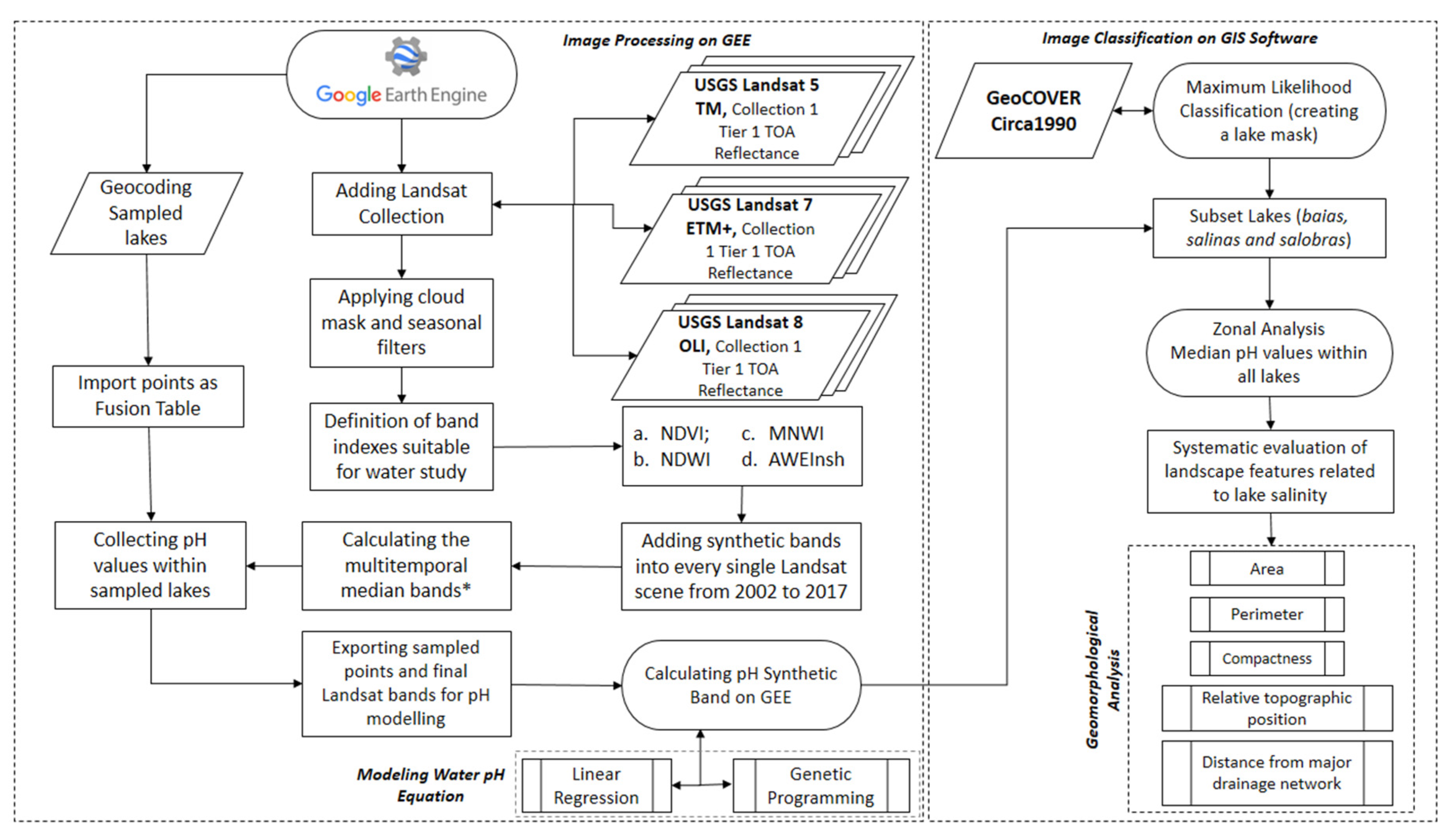
3. Dataset and Methods
3.1. Landsat Surface Reflectance Dataset
3.2. Water and Vegetation Indexes
3.3. Field Sample Data
3.4. Prediction of pH Values
3.5. Analyzing the Spatial Distribution of Saline and Freshwater Lakes
4. Results and Discussion
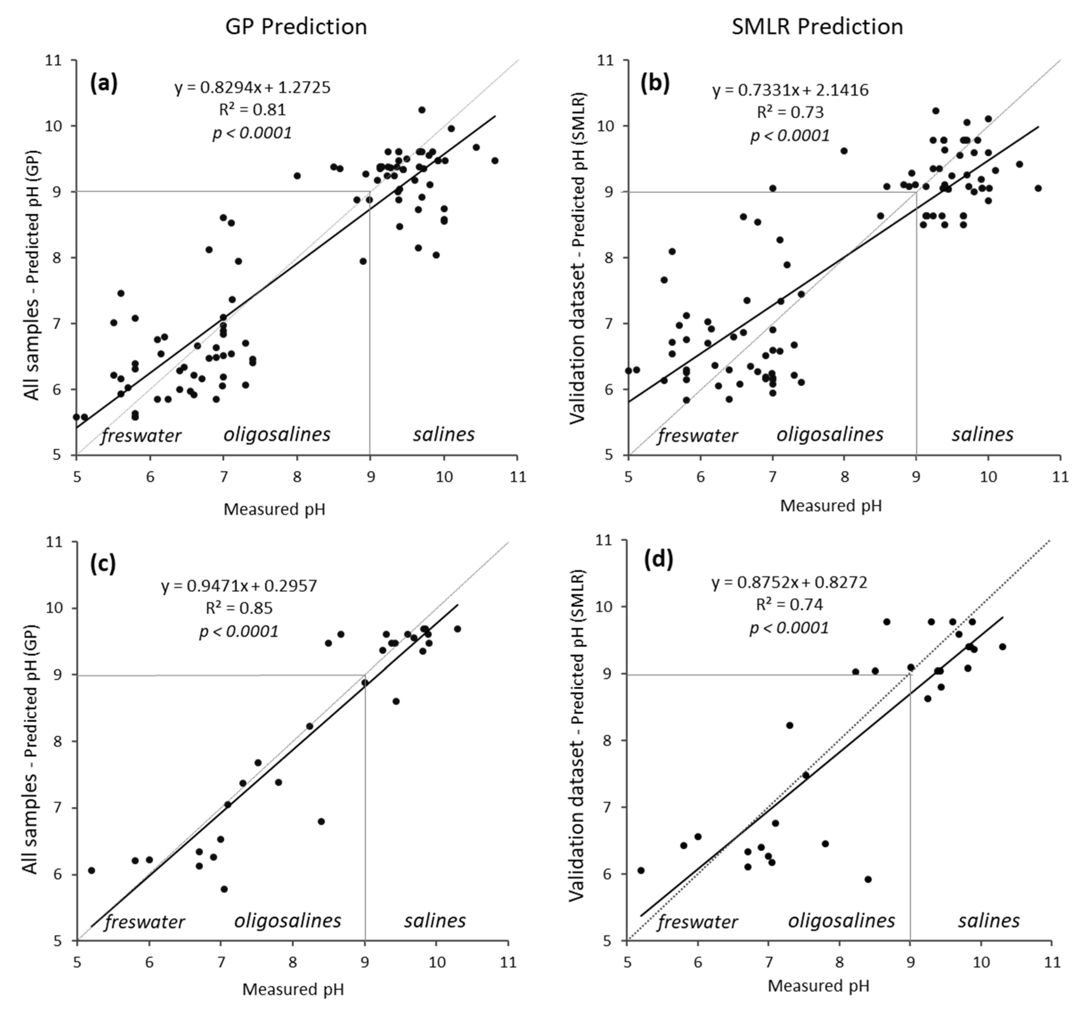
4.1. Spatial Modeling of Nhecolândia Lakes
Regression Models for Predicting pH in Lakes
4.2. Landscape Features Related to the Distribution of Lakes in the Nhecolândia
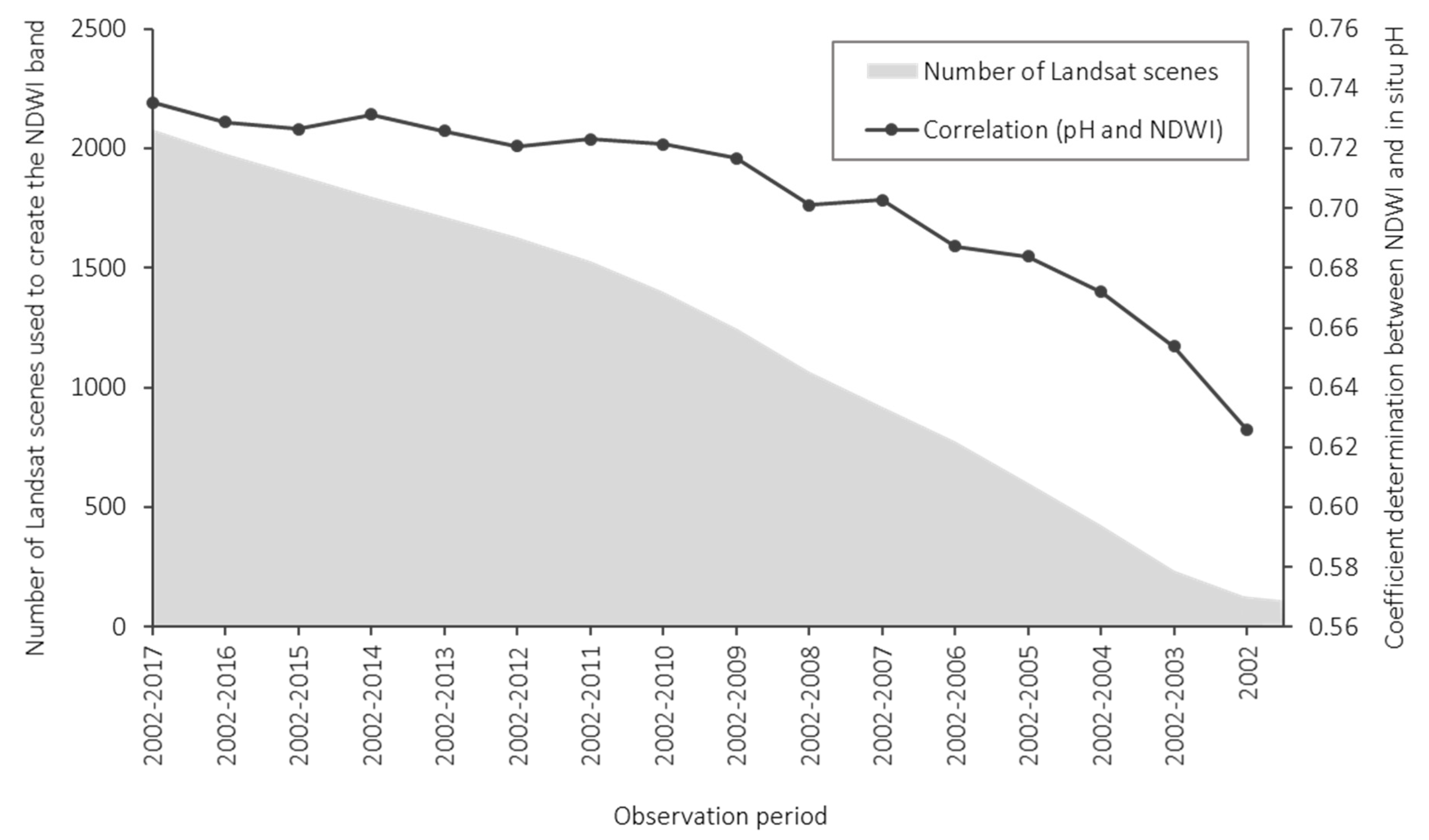
4.3. Remote Sensing Big Data for Inland Environments
5. Conclusions
Supplementary Materials
Author Contributions
Funding
Acknowledgments
Conflicts of Interest
References
- Löffler, H. The origin of lake basins. In The Lakes Handbook; O’Sullivan, P.E., Reynolds, C.S., Eds.; Blackwell Science: Oxford, UK, 2004; Volume 1, pp. 8–60. [Google Scholar]
- Hutchinson, G.E. A Treatise on Limnology. I. Geography, Physics, and Chemistry; John Wiley & Sons: New York, New York, USA, 1957; 1015p. [Google Scholar]
- Wetzel, R.G. Limnology: Lake and River Ecosystems; Gulf Professional Publishing: San Diego, CA, USA, 2001; 1014p. [Google Scholar]
- Winter, T.C. The Hydrology of Lakes. In The Lakes Handbook; O’Sullivan, P.E., Reynolds, C.S., Eds.; Blackwell Science: Oxford, UK, 2004; Volume 1, pp. 61–78. [Google Scholar]
- Lo, E.L.; McGlue, M.M.; Silva, A.; Bergier, I.; Yeager, K.M.; de Azevedo Macedo, H.; Swallom, M.; Assine, M.L. Fluvio-lacustrine sedimentary processes and landforms on the distal Paraguay fluvial megafan (Brazil). Geomorphology 2019, 342, 163–175. [Google Scholar] [CrossRef]
- Stevaux, J.C.; Macedo, H.d.A.; Assine, M.L.; Silva, A. Changing fluvial styles and backwater flooding along the Upper Paraguay River plains in the Brazilian Pantanal wetland. Geomorphology 2020, 350, 106906. [Google Scholar] [CrossRef]
- Furian, S.; Martins, E.R.C.; Parizotto, T.M.; Rezende-Filho, A.T.; Victoria, R.L.; Barbiero, L. Chemical diversity and spatial variability in myriad lakes in Nhecolândia in the Pantanal wetlands of Brazil. Limnol. Oceanogr. 2013, 58, 2249–2261. [Google Scholar] [CrossRef]
- Por, F.D. The Pantanal of Mato Grosso (Brazil): World’s Largest Wetlands; Springer Science & Business Media: Dordrecht, Netherlands, 1995; Volume 73. [Google Scholar]
- Keddy, P.A.; Fraser, L.H.; Solomeshch, A.I.; Junk, W.J.; Campbell, D.R.; Arroyo, M.T.; Alho, C.J. Wet and wonderful: The world’s largest wetlands are conservation priorities. BioScience 2009, 59, 39–51. [Google Scholar] [CrossRef] [Green Version]
- Assine, M.L.; Merino, E.R.; Pupim, F.N.; Macedo, H.A.; Santos, M.G.M. The Quaternary alluvial systems tract of the Pantanal Basin, Brazil. Braz. J. Geol. 2015, 45, 475–489. [Google Scholar] [CrossRef] [Green Version]
- Galvão, L.S.; Pereira Filho, W.; Abdon, M.M.; Novo, E.M.M.L.; Silva, J.S.V.; Ponzoni, F.J. Spectral reflectance characterization of shallow lakes from the Brazilian Pantanal wetlands with field and airborne hyperspectral data. Int. J. Remote Sens. 2003, 24, 4093–4112. [Google Scholar] [CrossRef]
- Costa, M.; Telmer, K.H.; Evans, T.L.; Almeida, T.I.; Diakun, M.T. The lakes of the Pantanal: Inventory, distribution, geochemistry, and surrounding landscape. Wetl. Ecol. Manag. 2015, 23, 19–39. [Google Scholar] [CrossRef]
- Almeida, T.I.R.; Calijuri, M.d.C.; Falco, P.B.; Casali, S.P.; Kupriyanova, E.; Paranhos Filho, A.C.; Sigolo, J.B.; Bertolo, R.A. Biogeochemical processes and the diversity of Nhecolândia lakes, Brazil. Ann. Braz. Acad. Sci. 2011, 83, 391–407. [Google Scholar] [CrossRef] [PubMed] [Green Version]
- Almeida, T.I.R.; Sígolo, J.B.; Fernandes, E.; Queiroz-Neto, J.P.; Barbiero, L.; Sakamoto, A.Y. Proposta de classificação e gênese das lagoas da baixa Nhecolândia-MS com base em sensoriamento remoto e dados de campo. Braz. J. Geol. 2003, 33 (Suppl. 2), 83–90. [Google Scholar] [CrossRef]
- Almeida, F.F.M. Geology of the Midwest Matogrossense; Bulletin of the Division of Geology and Mineralogy; SERGRAF: Rio de Janeiro, Brazil, 1964; 123p. [Google Scholar]
- Klammer, C. Die Paläovüste des Pantanal von Mato Grosso und Die Pleistozäne Klimageschichte der Brasilianischen Randtropen. Ann. Geomorphol. 1982, 26, 393–416. [Google Scholar]
- Wilhelmy, H. Meander and embankment lakes of tropical lowland rivers. Ann. Geomorphol. 1958, 2, 27–54. [Google Scholar] [CrossRef]
- Braun, E.W. Cone aluvial do Taquari, unidade geomórfica marcante da planície quaternária do Pantanal. Braz. J. Geogr. 1977, 39, 164–180. [Google Scholar]
- Palmer, S.C.J.; Kutser, T.; Hunter, P.D. Remote sensing of inland waters: Challenges, progress and future directions. Remote Sens. Environ 2015, 157, 1–8. [Google Scholar] [CrossRef] [Green Version]
- Rezende-Filho, A.T.; Valles, V.; Furian, S.; Oliveira, C.M.S.C.; Ouardi, J.; Barbiero, L. Impacts of Lithological and Anthropogenic Factors Affecting Water Chemistry in the Upper Paraguay River Basin. J. Environ. Qual. 2015, 44, 1832–1842. [Google Scholar] [CrossRef]
- Rezende Filho, A.T.; Furian, S.; Victoria, R.L.; Mascré, C.; Valles, V.; Barbiero, L. Hydrochemical variability at the Upper Paraguay Basin and Pantanal wetland. Hydrol. Earth Syst. Sci. 2012, 16, 2723–2737. [Google Scholar] [CrossRef] [Green Version]
- Barbiero, L.; Berger, G.; Rezende Filho, A.T.; Meunier, J.-F.; Martins-Silva, E.R.; Furian, S. Organic Control of Dioctahedral and Trioctahedral Clay Formation in an Alkaline Soil System in the Pantanal Wetland of Nhecolândia, Brazil. PLoS ONE 2016, 11, e0159972. [Google Scholar] [CrossRef] [Green Version]
- Barbiero, L.; Queiroz Neto, J.P.; Ciornei, G.; Sakamoto, A.Y.; Capellari, B.; Fernandes, E.; Valles, V. Geochemistry of water and ground water in the Nhecolândia, Pantanal of Mato Grosso, Brazil: Variability and associated processes. Wetlands 2002, 22, 528–540. [Google Scholar] [CrossRef]
- Furquim, S.A.C.; Graham, R.C.; Barbiero, L.; de Queiroz Neto, J.P.; Vallès, V. Mineralogy and genesis of smectites in an alkaline-saline environment of pantanal wetland, Brazil. Clays Clay. Miner. 2008, 56, 579–595. [Google Scholar] [CrossRef]
- Furquim, S.A.C.; Graham, R.C.; Barbiero, L.; Queiroz Neto, J.P.; Vidal-Torrado, P. Soil mineral genesis and distribution in a saline lake landscape of the Pantanal Wetland, Brazil. Geoderma 2010, 154, 518–528. [Google Scholar] [CrossRef]
- Evans, T.L.; Costa, M. Landcover classification of the Lower Nhecolândia subregion of the Brazilian Pantanal Wetlands using ALOS/PALSAR, RADARSAT-2 and ENVISAT/ASAR imagery. Remote Sens. Environ. 2014, 128, 118–137. [Google Scholar] [CrossRef]
- Gorelick, N.; Hancher, M.; Dixon, M.; Ilyushchenko, S.; Thau, D.; Moore, R. Google Earth Engine: Planetary-scale geospatial analysis for everyone. Remote Sens. Environ. 2017, 202, 18–27. [Google Scholar] [CrossRef]
- Casu, F.; Manunta, M.; Agram, P.S.; Crippen, R.E. Big Remotely Sensed Data: Tools, applications and experiences. Remote Sens. Environ. 2017, 202, 1–2. [Google Scholar] [CrossRef]
- Andreote, A.P.D.; Dini-Andreote, F.; Rigonato, J.; Machineski, G.S.; Souza, B.C.E.; Barbiero, L.; Rezende-Filho, A.T.; Fiore, M.F. Contrasting the Genetic Patterns of Microbial Communities in Soda Lakes with and without Cyanobacterial Bloom. Front. Microbiol. 2018, 9. [Google Scholar] [CrossRef] [Green Version]
- Barbiero, L.; Siqueira Neto, M.; Braz, R.R.; Carmo, J.B.; Rezende-Filho, A.T.; Mazzi, E.; Fernandes, F.A.; Damatto, S.R.; Camargo, P.B. Biogeochemical diversity, O2-supersaturation and hot moments of GHG emissions from shallow alkaline lakes in the Pantanal of Nhecolândia, Brazil. Sci. Total Environ. 2018, 619–620, 1420–1430. [Google Scholar] [CrossRef] [PubMed]
- Assine, M.; Merino, E.; Pupim, F.; Warren, L.; Guerreiro, R.; McGlue, M. Geology and Geomorphology of the Pantanal Basin. In The Handbook of Environmental Chemistry; Springer: Berlin/Heidelberg, Germany, 2015; pp. 1–28. [Google Scholar] [CrossRef] [Green Version]
- Bergier, I. Effects of highland land-use over lowlands of the Brazilian Pantanal. Sci. Total Environ. 2013, 463–464, 1060–1066. [Google Scholar] [CrossRef]
- Assine, M.L. River avulsions on the Taquari megafan, Pantanal wetland, Brazil. Geomorphology 2005, 70, 357–371. [Google Scholar] [CrossRef]
- Buehler, H.A.; Weissmann, G.S.; Scuderi, L.A.; Hartley, A.J. Spatial and temporal evolution of an avulsion on the Taquari River distributive fluvial system from satellite image analysis. J. Sediment Res. 2011, 81, 630–640. [Google Scholar] [CrossRef]
- Assine, M.L. Sedimentation in the Pantanal Sedimentar Basin, West-Central Brazil. Ph.D. Thesis, São Paulo State University, Rio Claro, Brazil, 2003. [Google Scholar]
- Hamilton, S.K.; de Souza, O.C.; Coutinho, M.E. Dynamics of floodplain inundation in the alluvial fan of the Taquari River (Pantanal, Brazil). SIL Proc. 1922–2010 1998, 26, 916–922. [Google Scholar] [CrossRef]
- Alvares, C.A.; Stape, J.L.; Sentelhas, P.C.; de Moraes, G.; Leonardo, J.; Sparovek, G. Köppen’s climate classification map for Brazil. Meteorol. J. 2013, 22, 711–728. [Google Scholar] [CrossRef]
- Alho, C.J.R. The Pantanal. In The World’s Largest Wetlands—Ecology and Conservation; Fraser, L.H., Keddy, P.A., Eds.; Cambridge University Press: New York, NY, USA, 2005; pp. 203–271. [Google Scholar]
- Zhou, L.; Lau, K.M. Does a Monsoon Climate Exist over South America? J. Clim. 1998, 11, 1020–1040. [Google Scholar] [CrossRef]
- Garreaud, R.D.; Vuille, M.; Compagnucci, R.; Marengo, J. Present-day South American climate. Palaeogeogr. Palaeoclimatol. Palaeoecol. 2009, 281, 180–195. [Google Scholar] [CrossRef]
- Assine, M.; Macedo, H.; Stevaux, J.; Bergier, I.; Padovani, C.; Silva, A. Avulsive Rivers in the Hydrology of the Pantanal Wetland. In Dynamics of the Pantanal Wetland in South America. The Handbook of Environmental Chemistry; Bergier, I., Assine, M.L., Eds.; Springer: Berlin/Heidelberg, Germany, 2015; pp. 83–110. [Google Scholar] [CrossRef] [Green Version]
- Junk, J.W.; Bayley, P.B.; Sparks, R.E. The flood pulse concept in river floodplain systems. Can. Spec. Publ. Fish. Aquat. Sci. 1989, 106, 110–127. [Google Scholar]
- Plink-Björklund, P. Morphodynamics of rivers strongly affected by monsoon precipitation: Review of depositional style and forcing factors. Sediment. Geol. 2015, 323, 110–147. [Google Scholar] [CrossRef] [Green Version]
- Hamilton, S.; Sippel, S.; Melack, J. Inundation patterns in the Pantanal wetland of South America determined from passive microwave remote sensing. Fundam. Appl. Limnol. 1996, 137, 1–23. [Google Scholar]
- Guerreiro, R.L.; McGlue, M.M.; Stone, J.R.; Bergier, I.; Parolin, M.; da Silva Caminha, S.A.F.; Warren, L.V.; Assine, M.L. Paleoecology explains Holocene chemical changes in lakes of the Nhecolândia (Pantanal-Brazil). Hydrobiologia 2017, 815, 1–29. [Google Scholar] [CrossRef] [Green Version]
- McGlue, M.M.; Guerreiro, R.L.; Bergier, I.; Silva, A.; Pupim, F.N.; Oberc, V.; Assine, M.L. Holocene stratigraphic evolution of saline lakes in Nhecolândia, southern Pantanal wetlands (Brazil). Quat. Res. 2017, 88, 472–490. [Google Scholar] [CrossRef]
- Costa, M.P.F.; Telmer, K.H. Utilizing SAR imagery and aquatic vegetation to map fresh and brackish lakes in the Brazilian Pantanal wetland. Remote Sens. Environ. 2006, 105, 204–213. [Google Scholar] [CrossRef]
- Barbiero, L.; Filho, A.R.; Furquim, S.A.C.; Furian, S.; Sakamoto, A.Y.; Valles, V.; Graham, R.C.; Fort, M.; Ferreira, R.P.D.; Neto, J.P.Q. Soil morphological control on saline and freshwater lake hydrogeochemistry in the Pantanal of Nhecolândia, Brazil. Geoderma 2008, 148, 91–106. [Google Scholar] [CrossRef] [Green Version]
- Masek, J.; Vermote, E.F.; Saleous, N.; Wolfe, R.; Hall, F.G.; Huemmrich, F.; Lim, T.K. LEDAPS Calibration, Reflectance, Atmospheric Correction Preprocessing Code, Version 2. Oak Ridge National Laboratory Distributed Active Archive Center, 2012. Available online: https://doi.org/10.3334/ORNLDAAC/1146 (accessed on 22 August 2019).
- U.S.G.S. USGS EarthExplorer. USGS Science for a Changing World. 2015. Available online: http://earthexplorer.usgs.gov/ (accessed on 1 July 2019).
- Zhu, Z.; Wang, S.; Woodcock, C.E. Improvement and expansion of the Fmask algorithm: Cloud, cloud shadow, and snow detection for Landsats 4–7, 8, and Sentinel 2 images. Remote Sens. Environ 2015, 159, 269–277. [Google Scholar] [CrossRef]
- Ivits, E.; Cherlet, M.; Sommer, S.; Mehl, W. Addressing the complexity in non-linear evolution of vegetation phenological change with time-series of remote sensing images. Ecol. Indic. 2013, 26, 49–60. [Google Scholar] [CrossRef]
- Hem, J.D. Study and Interpretation of the Chemical Characteristics of Natural Water, 3rd ed.; US Geological Survey: Alexandria, VA, USA, 1985; pp. 28–30.
- Meybeck, M.; Helmer, R. Introduction. In Water Quality Assessments. A Guide to the Use of Biota, Sediments and Water in Environmental Monitoring, 2nd ed.; Chapman, D., Ed.; CRC Press: London, UK, 1996. [Google Scholar]
- Tucker, C.J. Red and photographic infrared linear combinations for monitoring vegetation. Remote Sens. Environ 1979, 8, 127–150. [Google Scholar] [CrossRef] [Green Version]
- Feyisa, G.L.; Meilby, H.; Fensholt, R.; Proud, S.R. Automated Water Extraction Index: A new technique for surface water mapping using Landsat imagery. Remote Sens. Environ. 2014, 140, 23–35. [Google Scholar] [CrossRef]
- McFeeters, S.K. The use of the Normalized Difference Water Index (NDWI) in the delineation of open water features. Int. J. Remote Sens. 1996, 17, 1425–1432. [Google Scholar] [CrossRef]
- Xu, H. Modification of normalised difference water index (NDWI) to enhance open water features in remotely sensed imagery. Int. J. Remote Sens. 2006, 27, 3025–3033. [Google Scholar] [CrossRef]
- Koza, J.R. Evolving a Computer Program to Generate Random Numbers Using the Genetic Programming Paradigm. In Proceedings of the 4th International Conference on Genetic Algorithms, San Diego, CA, USA, July 1991. [Google Scholar]
- Schmidt, M.; Lipson, H. Symbolic Regression of Implicit Equations. In Genetic Programming Theory and Practice VII; Riolo, R., O’Reilly, U.-M., McConaghy, T., Eds.; Springer US: Boston, MA, USA, 2010; pp. 73–85. [Google Scholar] [CrossRef] [Green Version]
- Parinet, B.; Lhote, A.; Legube, B. Principal component analysis: An appropriate tool for water quality evaluation and management—application to a tropical lake system. Ecol Modell. 2004, 178, 295–311. [Google Scholar] [CrossRef]
- MDA Federal, 2004. Landsat GeoCover 1990/TM Edition Mosaics. Tile S-21-15. ETM-EarthSat-MrSID, 1.0. USGS: Sioux Falls, SD, USA, 1990. Available online: https://landsatlook.usgs.gov/ (accessed on 1 July 2019).
- Takaku, J.; Tadono, T.; Tsutsui, K. Generation of high resolution global DSM from ALOS Prism. Int. Arch. Photogramm. Remote Sens. Spatial Inf. Sci. 2014, XL-4, 243–248. [Google Scholar] [CrossRef] [Green Version]
- Zani, H.; Assine, M.L.; McGlue, M.M. Remote sensing analysis of depositional landforms in alluvial settings: Method development and application to the Taquari megafan, Pantanal (Brazil). Geomorphology 2012, 161, 82–92. [Google Scholar] [CrossRef]
- Martins, E.R.C. Typology of Saline Lakes in the Pantanal of Nhecolândia (MS). Ph.D. Thesis, University of São Paulo, São Paulo, Brazil, 2012. [Google Scholar]
- Merino, E.R.; Assine, M.L. Hidden in plain sight: How finding a lake in the Brazilian Pantanal improves understanding of wetland hydrogeomorphology. Earth Surf Process Landf. 2019, 45, 440–458. [Google Scholar] [CrossRef]
- Pott, A.; da Silva, J.S.V. Terrestrial and aquatic vegetation diversity of the Pantanal wetland. In Dynamics of the Pantanal Wetland in South America; Bergier, I., Assine, M.L., Eds.; Springer International Publishing: Cham, Switzerland, 2015; pp. 111–131. [Google Scholar] [CrossRef]
- Freitas, J.G.; Furquim, S.A.C.; Aravena, R.; Cardoso, E.L. Interaction between lakes’ surface water and groundwater in the Pantanal wetland, Brazil. Environ. Earth Sci. 2019, 78, 139. [Google Scholar] [CrossRef]
- Andreote, A.P.D.; Vaz, M.G.M.V.; Genuário, D.B.; Barbiero, L.; Rezende-Filho, A.T.; Fiore, M.F. Nonheterocytous cyanobacteria from Brazilian saline-alkaline lakes. J. Phycol. 2014, 50, 675–684. [Google Scholar] [CrossRef]
- Park, E.; Latrubesse, E.M. Modeling suspended sediment distribution patterns of the Amazon River using MODIS data. Remote Sens. Environ. 2014, 147, 232–242. [Google Scholar] [CrossRef]
- Zang, C.; Huang, S.; Wu, M.; Du, S.; Scholz, M.; Gao, F.; Guo, Y.; Dong, Y. 2011. Comparison of Relationships Between pH, Dissolved Oxygen and Chlorophyll a for Aquaculture and Non-aquaculture Waters. Water Air Soil Pollut. 2011, 219, 157–174. [Google Scholar] [CrossRef]
- Mariot, M.; Dudal, Y.; Furian, S.; Sakamoto, A.; Vallès, V.; Fort, M.; Barbiero, L. Dissolved organic matter fluorescence as a water-flow tracer in the tropical wetland of Pantanal of Nhecolândia, Brazil. Sci. Total Environ. 2007, 388, 184–193. [Google Scholar] [CrossRef] [PubMed] [Green Version]
- Duarte, C.M.; Prairie, Y.T.; Montes, C.; Cole, J.J.; Striegl, R.; Melack, J.; Downing, J.A. CO2 emissions from saline lakes: A global estimate of a surprisingly large flux. J. Geophys. Res. Biogeosci. 2008, 113. [Google Scholar] [CrossRef] [Green Version]
- Martins, E.R.C.; Furian, S.; Barbiero, L. Dynamic of Lake Morphology on the Taquari Alluvial Fan: Pantanal of Nhecolândia (Ms), Brazil. In Proceedings of the VII National Congress of Geomorphology, Lisboa, Portugal, 8–10 October 2015. [Google Scholar]
- Carpenter, D.J.; Carpenter, S.M. Modeling inland water quality using Landsat data. Remote Sens. Environ. 1983, 13, 345–352. [Google Scholar] [CrossRef]
- Gallie, E.A.; Murtha, P.A. A modification of chromaticity analysis to separate the effects of water quality variables. Remote Sens. Environ. 1993, 44, 47–65. [Google Scholar] [CrossRef]
- Barnes, B.B.; Hu, C.; Holekamp, K.L.; Blonski, S.; Spiering, B.A.; Palandro, D.; Lapointe, B. Use of Landsat data to track historical water quality changes in Florida Keys marine environments. Remote Sens. Environ. 2014, 140, 485–496. [Google Scholar] [CrossRef]
- Thomann, G.C. Remote measurement of salinity in an estuarine environment. Remote Sens. Environ 1971, 2, 249–259. [Google Scholar] [CrossRef]
- Khorram, S. Remote sensing of salinity in the San Francisco Bay Delta. Remote Sens. Environ 1982, 12, 15–22. [Google Scholar] [CrossRef]
- Scudiero, E.; Skaggs, T.H.; Corwin, D.L. Regional scale soil salinity evaluation using Landsat 7, western San Joaquin Valley, California, USA. Geoderma Reg. 2014, 2–3, 82–90. [Google Scholar] [CrossRef]
- Muller, S.J.; van Niekerk, A. An evaluation of supervised classifiers for indirectly detecting salt-affected areas at irrigation scheme level. Int. J. Appl. Earth Obs. Geoinf. 2016, 49, 138–150. [Google Scholar] [CrossRef]
- Gorji, T.; Sertel, E.; Tanik, A. Monitoring soil salinity via remote sensing technology under data scarce conditions: A case study from Turkey. Ecol. Indic. 2017, 74, 384–391. [Google Scholar] [CrossRef]
- Zhang, T.-T.; Qi, J.-G.; Gao, Y.; Ouyang, Z.-T.; Zeng, S.-L.; Zhao, B. Detecting soil salinity with MODIS time series VI data. Ecol. Indic. 2015, 52, 480–489. [Google Scholar] [CrossRef]
- El Harti, A.; Lhissou, R.; Chokmani, K.; Ouzemou, J.; Hassouna, M.; Bachaoui, E.M.; El Ghmari, A. Spatiotemporal monitoring of soil salinization in irrigated Tadla Plain (Morocco) using satellite spectral indices. Int. J. Appl. Earth Obs. Geoinf. 2016, 50, 64–73. [Google Scholar] [CrossRef]


| SMLR GEE Collections | Adjusted R2 | RMSE | AIC | Considered Bands |
|---|---|---|---|---|
| Full Collection (2002 to 2017) | 0.68 | 0.82 | −12.91 | B1/B2/B3/B7/MNDWI/NDWI |
| High Water Season Jan to May (2002 to 2017) | 0.72 | 0.90 | −37.18 | B1/B4/B5/MNDWI/NDWI |
| Low Water Season Jul to Out (2002 to 2017) | 0.65 | 0.94 | −8.15 | B1/B2/B3/B4/MNDWI |
| High Water (2014 to 2017 field samples) | 0.64 | 0.96 | −3.03 | B1/B3/B4/B7/NDVI/NDWI |
| High Water (2008 field samples) | 0.67 | 0.92 | −13.2 | B1/B2/B4/B5/NDVI/NDWI |
© 2020 by the authors. Licensee MDPI, Basel, Switzerland. This article is an open access article distributed under the terms and conditions of the Creative Commons Attribution (CC BY) license (http://creativecommons.org/licenses/by/4.0/).
Share and Cite
Pereira, O.J.R.; Merino, E.R.; Montes, C.R.; Barbiero, L.; Rezende-Filho, A.T.; Lucas, Y.; Melfi, A.J. Estimating Water pH Using Cloud-Based Landsat Images for a New Classification of the Nhecolândia Lakes (Brazilian Pantanal). Remote Sens. 2020, 12, 1090. https://doi.org/10.3390/rs12071090
Pereira OJR, Merino ER, Montes CR, Barbiero L, Rezende-Filho AT, Lucas Y, Melfi AJ. Estimating Water pH Using Cloud-Based Landsat Images for a New Classification of the Nhecolândia Lakes (Brazilian Pantanal). Remote Sensing. 2020; 12(7):1090. https://doi.org/10.3390/rs12071090
Chicago/Turabian StylePereira, Osvaldo J. R., Eder R. Merino, Célia R. Montes, Laurent Barbiero, Ary T. Rezende-Filho, Yves Lucas, and Adolpho J. Melfi. 2020. "Estimating Water pH Using Cloud-Based Landsat Images for a New Classification of the Nhecolândia Lakes (Brazilian Pantanal)" Remote Sensing 12, no. 7: 1090. https://doi.org/10.3390/rs12071090