Generalised Regression Hypothesis Induction for Energy Consumption Forecasting

Abstract

This work addresses the problem of energy consumption time series forecasting. In our approach, a set of time series containing energy consumption data is used to train a single, parameterised prediction model that can be used to predict future values for all the input time series. As a result, the proposed method is able to learn the common behaviour of all time series in the set (i.e., a fingerprint) and use this knowledge to perform the prediction task, and to explain this common behaviour as an algebraic formula. To that end, we use symbolic regression methods trained with both single- and multi-objective algorithms. Experimental results validate this approach to learn and model shared properties of different time series, which can then be used to obtain a generalised regression model encapsulating the global behaviour of different energy consumption time series.

1. Introduction

Energy efficiency in the building sector has become an important research area for two main reasons: firstly, because the residential sector represents around 25% of global energy consumption; and secondly, because the building sector is also considered as the main contributor to the energy shortage and climate change effects regarding the worldwide increased population and the large environmental impacts [1,2]. Building infrastructures include sensor technologies [3] that provide a huge amount of energy consumption data that allows researchers to address the problem of energy usage and its environmental impact from different perspectives [4], such as anomaly detection [5,6], energy consumption modelling [7,8], energy demand planning [9] or consumer profile mining [10,11].

Each of these problems has been addressed with different techniques, according to the nature of the problem and the desired output. For instance, in anomaly detection problems, Chou and Telaga [5] used a neural network to predict the energy consumption of future days and attempted to detect the energy consumption anomalies identifying the differences between the real and predicted energy data. On the other hand, Cui and Wang [6] proposed a hybrid model that combines polynomial regressions and Gaussian distributions to build data detection and visualisation systems that help to identify anomalies in electricity consumption data. Regarding consumer profile problems, Gomez et al. [10] used a data-fitting approach and a multi-class classifier to estimate the electricity needed in a building, and Capozzoli et al. [11] used pattern recognition and classification algorithms to provide knowledge about the energy usage in a building. Regarding energy consumption modelling, Zhao et al. [12] used occupant information in addition to the heating, ventilation and air conditioning (HVAC) energy consumption data to determine the pollution impact of buildings. As another example, Balaji et al. [13] built a control system that uses the WiFi network traffic in a building to estimate the occupancy and control the HVAC. Due to the heterogeneous nature of the different sources of data, every approach usually needs a preprocessing stage to provide useful data to the models, as argued in [7].

Our current work focuses on energy consumption forecasting in public buildings. Traditionally, energy consumption forecasting in residential and public buildings has been implemented by means of analysing a single energy consumption time series [14,15,16,17,18]. In these cases, this single time series is given as input to a prediction model, with the potential addition of some external data (temperature, building occupancy, etc.). These models have proven able to provide suitable results in their respective case studies, obtaining accurate prediction models. On the other hand, there are many works that combine historical energy data with statistical and machine learning techniques to provide more accurate models able to improve the energy consumption in buildings.

A good and recent review on this topic [19] summarises the state of the art in the energy consumption forecasting paradigm, and describes the most used techniques to that end. To only cite a few, Yasmin et al. developed ARIMA models (Autorregresive Intregrated Moving Average) [20] to predict electricity consumption in Pakistan and Baca Ruiz et al. [21] proposed nonlinear autoregressive artificial neural networks with exogenous inputs (NARX) to predict the energy consumption in public buildings. There is a plethora of proposals in the literature for energy consumption forecasting in the last few years, and a complete survey paper would be necessary to analyse all these research approaches.

Unlike traditional approaches in energy consumption forecasting for buildings, which use a single time series that contains historical data of energy consumption and exogenous information, we address our research from a different perspective and we assume that there are multiple buildings whose energy consumption must be predicted. We hypothesise that, if the energy consumption of different buildings is medium or highly correlated, then these buildings share the same energy consumption ground behaviour. Then, our goal is to obtain a general forecasting model able to learn structural relationships of all time series in a set, and to parameterise this model for its particular adaptation for each specific building, obtaining a more accurate prediction model that explains the overall energy consumption behaviour of the whole compound.

To address this problem, we use symbolic regression and genetic algorithms to find interpretable regression models that describe the relationships in the energy consumption data that are common to all buildings under study in a compound. More specifically, we assume that each related building provides a dataset with their energy consumption, and our motivation is to find a general regression hypothesis f able to explain all datasets of each building. These regression models will then be parameterised for its adaptation to a specific building forecasting task. As we have not found any work in the literature that solves a similar problem, we attempt to use two alternatives, namely classical genetic algorithms and multi-objective optimisation approaches, to identify the strengths and weaknesses of each type of techniques. In addition, in the experiments, we firstly validated the approach with synthetic data generated in the laboratory, and then in a real scenario. In both cases, we departed from several energy consumption time series that are medium or highly correlated, and we attempted to find a single regression model able to learn the shared ground behaviour of all these data series. The ultimate goal was to predict their future values accurately with the same model, parameterised for each data series.

To achieve these objectives, this manuscript is organised as follows. Section 2 introduces the fundamentals of symbolic regression and the different historical alternatives used to solve multi-objective problems. After that, Section 3 describes the formulation of the problem and the proposed methods. Section 4 shows the experimental results in two scenarios: synthetic data generated in the laboratory and real energy consumption data. Finally, conclusions and future works are described in Section 5.

2. Related Work

The literature gathers several techniques able to solve energy forecasting problems, such as neural networks [22,23], support vector machines, decision trees [24,25] or regression analysis techniques [26,27]. Since we were interested in finding not only accurate but also interpretable solutions for the final user, we focus this research in regression analysis techniques, and study their limitations and the solutions provided by different authors in the literature in Section 2.1. After that, we establish the basic concepts of multi-objective optimisation techniques required for our research in Section 2.2.

2.1. Symbolic Regression

Regression analysis is a classical tool widely used by researchers in prediction and data modelling problems. Given an algebraic expression f as model hypothesis, a set of input data (independent variables) $\overline{x}=(x_1,x_2,\dots ,x_n)$ and output data (dependent variables) $\overline{y}=(y_1,y_2,\dots ,y_m)$, the regression analysis attempts to find the optimal model parameters $\overline{w}=(w_1,w_2,\dots ,w_k)$ such as $\overline{y}=f(\overline{x},\overline{w})$, where $x_i,y_j,w_l\in \mathbb{R},\forall i,j,l:1\le i\le n,1\le j\le m,1\le l\le k$. The parameters $\overline{w}$ are usually found using numerical procedures, such as least squares optimisation, that minimise an error measurement, for instance $e(f(\overline{x},\overline{w}),\overline{y})=\left|\right|f(\overline{x},\overline{w})-\overline{y}\left|\right|$. However, the main limitation of traditional regression analysis appears when not only the parameters $\overline{w}$ are unknown, but also the model hypothesis f, or when f is very difficult to formulate manually. To solve this limitation, symbolic regression [28] combines a set of predefined atomic operators (such as +, -, *, /, and sin), independent variables $\overline{x}$ and parameters $\overline{w}$ to build an algebraic expression $\tilde{f}$ as an approximation for the optimal model f. To do so, symbolic regression uses optimisation algorithms to explore the search space and finds the best approximation $\tilde{f}$ that minimises an error measure, such as $\left|\right|\overline{y}-\tilde{f}(\overline{x},\overline{w})\left|\right|$.

Although there are many techniques designed to solve optimisation problems, we chose genetic programming due to its demonstrated potential in several areas [29], including symbolic regression. Genetic programming [30] is a supervised machine learning method based on biological evolution and is used in symbolic regression problems since it evolves a population of candidate algebraic expressions $\tilde{f}(\overline{x},\overline{w})$ and applies a set of genetic operators [31] to obtain the best candidate $\tilde{f}$. Although tree structures are highly used to encode the algebraic expressions of the population in genetic programming algorithms, our previous research [32] has demonstrated that alternative representations such as Straight Line Programs (SLP) are able to improve the solutions of symbolic regression problems in terms of not only accuracy and computational time but also obtaining more interpretable algebraic expressions.

Symbolic regression has been proposed previously as a tool to model energy consumption. The state of the art in this topic includes the work by Yang et al. [33], who used symbolic regression and evolutionary algorithms to identify the main factors in the energy consumption in China. Whereas Bhattacharya et al. [34] used linear genetic programming to perform consumer electricity demand forecasting, Behera et al. [35] used a genetic algorithm in order to develop an effective planning system able to estimate demand and energy consumption. In our works, we have also studied the use of symbolic regression for energy consumption modelling with good results [32].

Benefits of symbolic regression for energy consumption prediction are the simplicity of the resulting models, in contrast to more complex and difficult to analyse models such as neural networks or support vector machines, and also their interpretability by a non-expert in machine learning. On the other hand, limitations arise in the side of accuracy when dependencies between input and output data are difficult to find. In these cases, universal approximators such as neural networks have shown good performance [21]. Overall, we have selected symbolic regression as representation of forecasting model hypotheses due to the balance between their easy interpretability and good accuracy.

2.2. Multi-Objective Optimisation Paradigm

As previously described, our goal is to obtain a single general and parameterised forecasting model able to predict the energy consumption of different buildings. Thus, given a set of N energy consumption time series as input (one for each building), the task at hand is to find a unique parameterised regression model $\tilde{f}(\overline{x^i},\overline{w^i})$ that consistently models and predict future values of each ith time series separately. If the values $\overline{y^i}$ are the desired outputs for forecasting the ith time series, then we can measure N prediction errors as $e(\tilde{f},i)=\left|\right|\overline{y^i}-\tilde{f}(\overline{x^i},\overline{w^i})\left|\right|$. Finding the desired model $\tilde{f}$ therefore requires the minimisation of the N error measurements separately. In this work we consider two approaches to address this problem: (1) a single-objective approach, where all error measurements are aggregated into an unique measurement as $e(\tilde{f})={\sum }_{i=1}^{N}e(\tilde{f},i)$; and (2) using multi-objective optimisation, where each error measurement $e(\tilde{f},i)$ would be considered as a separate target function to be minimised.

Multi-objective optimisation problems attempt to find models that minimise/maximise a set of objective measures simultaneously, and represent the solution of each objective in a vector function e. Formally, a multi-objective problem is defined as the minimisation of multiple criteria $e(\overline{x})=(e_1(\overline{x}),e_2(\overline{x}),\dots ,e_m(\overline{x}))$, where $\overline{x}=(x_1,x_2,\dots ,x_n)$ is the vector of decision variables, and $e(x)=(e_1,e_2,\dots ,e_m)$ are the objective functions that must be minimised/maximised. An important aspect to take into account solving a multi-objective problem is related with the problem statement. As Hassan [36] argued, a multi-objective problem can be addressed from three different perspectives: converting the multi-objective problem in a single-objective one [37,38,39], using population-based algorithms [39,40,41] and studying Pareto-optimal based techniques [42,43,44,45,46].

Multi-objective optimisation techniques have been used to solve energy consumption problems (e.g., [47,48,49,50]). Therefore, in this work, we compare single-objective and NSGA-II multi-objective approaches to train symbolic regression forecasting models. The next section describes the problem statement of each approach, the representation used to solve symbolic regression and the main components of the algorithmic procedure.

3. Methods

Our method is based on the assumption that there is a set of several datasets (time series) composed of input/output patterns with the same structure, for which we want to model the output data with respect to the input data and obtain an algebraic expression that models the input/output relationship. We also hypothesise that there is a shared ground common behavior that is present in all these datasets, and that can explain output data regarding input data (at least partially). The model for this shared behavior could be unknown in advance. Due to this assumption, we consequently expect a medium/high correlation between the output data of all datasets.

As a toy example to understand these hypotheses, we sampled data from two linear functions $y_1=f_1(x_1)=3*x_1+5+{ϵ}_1$, and $y_2=f_2(x_2)=6*x_2+1+{ϵ}_2$ (where ${ϵ}_1,{ϵ}_2$ stand for an error in each dataset, respectively) and obtained two datasets $(X_1,Y_1)$ and $(X_2,Y_2)$. Both datasets come from different data distributions, but share a common ground behavior that could explain $y_1$ from $x_1$ and $y_2$ from $x_2$, and could be written as $y=f(x)=a*x+b$. Thus, the regression hypothesis f can be used to explain both datasets, when it is parameterised by the coefficients a and b.

We could use traditional symbolic regression methods to solve this toy example, by means of solving each dataset separately, and probably obtaining algebraic expressions that match $f_1$ and $f_2$, respectively. In this article, we provide an automatic method to find general regression hypotheses that could help to explain multiple datasets, providing a single parameterised algebraic expression that model the common ground behavior of all datasets. A necessary constraint of our proposal is that all datasets must have the same data structure, i.e., they are composed by a set of independent (input) variables $X=(x_1,x_2,\dots ,x_k)$ where $x_m\in \mathbb{R},\forall m:1\le m\le k$, and the number of variables k is the same for all datasets, and a single dependent (output) variable $Y=(y_1)$ where $y_1\in \mathbb{R}$.

The problem formulation assumes a set of n datasets $(X_1,Y_1),(X_2,Y_2),\dots ,(X_n,Y_n)$ whose data have this structure, i.e., $X_i=(x_1^i,x_2^i,\dots ,x_k^i)$ and $Y_i=(y_1^i)$$\forall i:1\le i\le n$ are the input and output variables, respectively, of the ith dataset. We denote $N(i)=(X_i,Y_i)$ as the number of input/output patterns of the ith dataset. We remark that two datasets can have different sizes (number of input/output patterns), so that $N(i)$ can be different to $N(j)$ for two different datasets, without loss of generality. Thus, the main goal of this work consists of finding a general parameterised algebraic expression $F(X,W)$ able to explain the relationships between dependent (output) and independent (input) data from all datasets simultaneously, where $W=(w_1,w_2,\dots ,w_l):w_q\in \mathbb{R}\forall q:1\le q\le l$ is a set of parameters or coefficients estimated for each specific dataset. Finding the values for the parameters of each dataset, $W_i$, is also a component of the proposed method and implemented as a local search procedure within a genetic evolutionary approach. We deepen into the algorithms description in the following sections.

3.1. Straight Line Programs for Time Series Prediction

A time series is a sequence of data (that we call x) evenly sampled in time (t) that is used to predict futures values $x(t+k)$. The goal of time series prediction is to find a model f that combines h previous values of the time series data and parameters w, to forecast the next values of the time series as $x(t+1)=f(x(t),x(t-1),\dots ,x(t-h),w)$. The value h is usually called time horizon.

In this paper, we use symbolic regression to predict future values of energy consumption time series. By using symbolic regression, we assume that the prediction model f can be written as an algebraic expression. Although there are different alternatives to encode algebraic expressions, including trees and linear genetic programming, Straight Line Programs have proved their potential over classical representations [51]. Straight Line Programs (SLP) are represented as a sequence of grammar production rules, where each production rule is composed by a set of known mathematical operators $O_{U_i}\in \{o_1,o_2,\dots ,o_m\}$ (as for instance $\{+,-,*,/,sin,cos\}$), a set of terminal symbols $T=\{t_1,t_2,\dots ,t_k\}$ (as for instance, parameters $\overline{w}=\{w_1,w_2,\dots ,w_k\}$ or independent variables $\overline{x}=\{x_1,x_2,\dots ,x_n\}$) and references to other rows $R_{U_{i,1}},R_{U_{i,2}}\in \{T\cup \{U_1,U_2,\dots ,U_{i-1}\}\}$. We may verify that the production rules that appear in the consequent must be references to previous rules, in order to avoid recursion.

$$\left\{\begin{array}{c}{U}_1\to 2*x\hfill \\ U_2\to 8+U_1\hfill \\ U_3\to sin(U_2)\hfill \\ U_4\to U_3-U_2\hfill \\ U_5\to x*U_4\hfill \\ U_6\to U_2/U_5\hfill \end{array}\right.$$

(1)

We can build an algebraic expression from a SLP by evaluating the Nth rule, which is the starting symbol of the grammar $U_N$. As an example, Equation (1) gathers a SLP that encodes the algebraic expression $f(x,\overline{w})={\displaystyle \frac{w_1+(w_2*x)}{x*sin(w_1+(w_2*x))-w_1+(w_2*x)}}$, where $\overline{w}=(w_1,w_2)=(8,2)$.

The following subsections gather the problem formulation for each approach and also a description of the main genetic operators to train SLP representations using genetic algorithms.

3.2. Single-Objective Problem Formulation

The problem addressed in this research is applied over multiple time series simultaneously, and it assumes that symbolic regression should find a general algebraic expression $F(X,W)$ that models the dependent variables of several datasets simultaneously, where X represents the independent variables of the datasets and W is the set of parameters values estimated by symbolic regression. The single-objective formulation of the problem assumes that symbolic regression should minimise an error function $e(F)$ in order to find the general algebraic expression F. We calculate this error $e(F)$ as the sum of the errors of F of all datasets to approximate the desired output Y (Equation (2)).

$$e(F)=\sum _{i=1}^n({\displaystyle \frac{1}{N(i)}}*\sum _{p=1}^{N(i)}{(F(X_i(p),W_i)-Y_i(p))}^2)$$

(2)

where n stands for the number of datasets, $N(i)$ is the number of data samples of the ith dataset, $X_i(p)$ is the pth input sample of the ith dataset, $Y_i(p)$ is the pth output sample of the ith dataset, and $W_i$ are the values of the algebraic function parameters of the ith dataset. The optimisation problem is formulated as finding the algebraic expression $\tilde{F}=mi{n}_F(e(F))$. Once the problem is formulated as explained, we use a genetic algorithm to find a SLP that provides the best regression hypothesis $\tilde{F}$.

Using the previous formulation, the accuracy error of the prediction model F over a time series $X_i$ is aggregated into a single measurement $e(F)$. In contrast, the multi-objective formulation shown in the next section treats the error minimisation of each time series separately.

3.3. Multi-Objective Problem Formulation

The single objective problem formulation described in the previous section is likely to have limitations if datasets are not normalised, since $e(F)$ is defined as the sum of squared errors in all datasets. If the data scale varies significantly from one dataset to another, then the errors could also vary significantly, and then the datasets with higher absolute errors could dominate the search in the solution space. In cases in which the data cannot be normalised, or if we do not know lower and upper bounds to perform a normalisation, then the single objective strategy could lead us to obtain undesired local optima solutions. To solve this limitation, we also provide a problem formulation from a multi-objective optimisation perspective.

In it, we define a minimisation objective per each dataset, so we assume a set of n objectives $(O_1,O_2,\dots ,O_n)$, where each objective $O_i$ attempts to minimise the error function of the corresponding ith dataset $(X_i,Y_i)$. Therefore, in the searching process of the general algebraic expression F, the multi-objective approach attempts to minimise each objective individually, finding the function F that minimises the error of the ith objective without worsening the quality of the jth objective. In this way, this formulation may avoid local optima when the data are not normalised since bad solutions in the estimation of some datasets do not influence the exploration of the search space for the remaining objectives. Thus, the goal is to find a general algebraic expression F that minimises an error function $e(F,i)$ for each of the objectives. The error measurement that must be minimised for each objective is shown in Equation (3).

$$\begin{array}{cc}\hfill O_1& =e(F,1)={\displaystyle \frac{1}{N(1)}}*\sum _{p=1}^{N(1)}{(F(X_1(p),W_1)-Y_1(p))}^2\hfill \\ ⋮\hfill \\ \hfill O_i& =e(F,i)={\displaystyle \frac{1}{N(i)}}*\sum _{p=1}^{N(i)}{(F(X_i(p),W_i)-Y_i(p))}^2\hfill \\ ⋮\hfill \\ \hfill O_n& =e(F,n)={\displaystyle \frac{1}{N(n)}}*\sum _{p=1}^{N(n)}{(F(X_n(p),W_n)-Y_n(p))}^2\hfill \end{array}$$

(3)

where n stands for the number of objectives (i.e., the number of datasets), $N(i)$ is the number of data samples of the ith dataset, $X_i(p)$ is the pth input sample of the ith dataset, $Y_i(p)$ is the pth output sample of the ith dataset, and $W_i$ is the set of parameter values for the target algebraic expression F for the ith dataset. The multi-objective formulation of the problem is to find the optimal algebraic expression $\tilde{F}$, or the set of Pareto-optimal algebraic expressions $\tilde{F}$, such as $\tilde{F}=mi{n}_F(e(F,i))\forall 1\le i\le n$. Once the problem is formulated as explained, we train SLPs to minimise $(O_1,O_2,\dots ,O_n)$ using the multi-objective algorithm NSGA-II [46].

3.4. Algorithm Description

We use a classic genetic algorithm [32] to optimise the single-objective approach, and the NSGA-II [46] method for the multi-objective optimisation approach. Since no changes were made to these template algorithms, in this section, we only describe the genetic operators to be used with SLP representation. We also remark that both crossover and mutation operators were proposed by Alonso et al. [51] and we summarise the procedure of each operator with the aim of improving the understanding of this work.

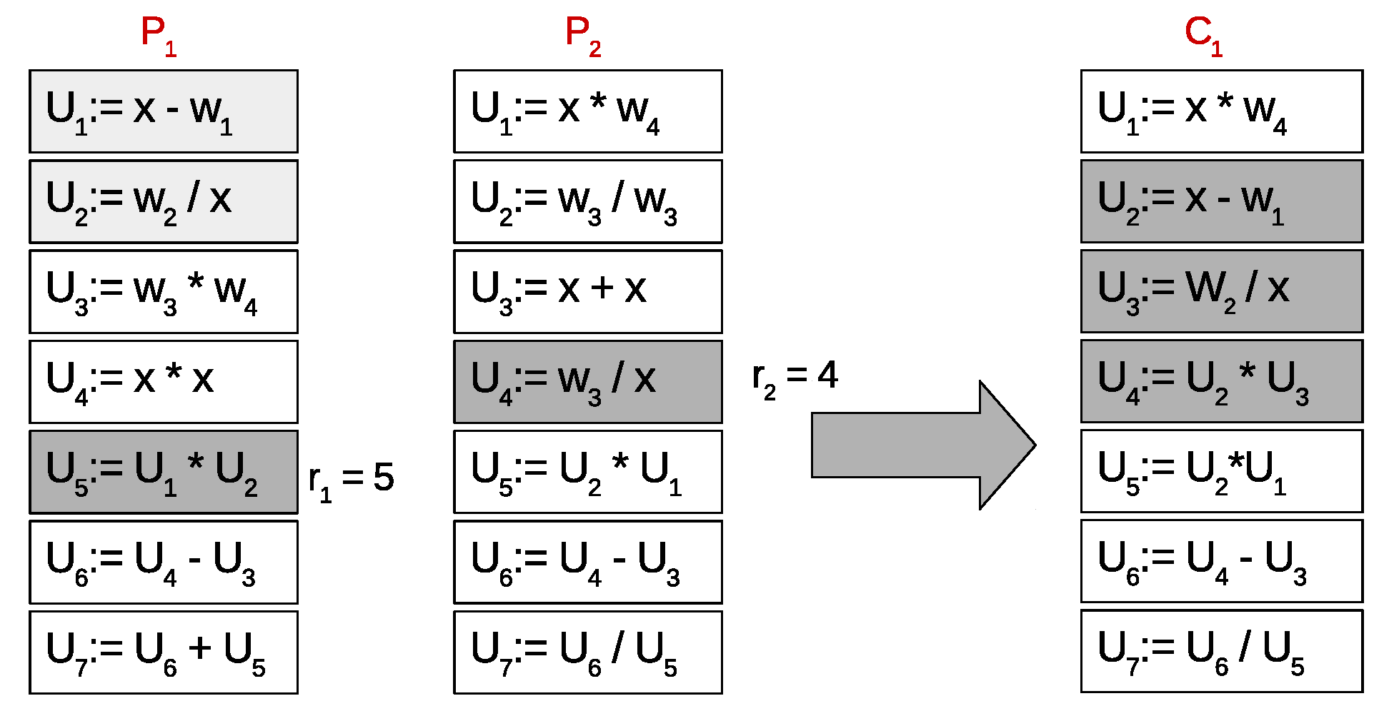
• Crossover operator. Two parents $P_1$ and $P_2$ are used in both single- and multi-objective approaches in order to generate two new children $C_1$ and $C_2$. The operator starts out selecting a random rule $U_i\in \{U_1,U_2,\dots ,U_{N-1}\}$ from $P_1$. After that, an ordered set of rules R is calculated as the set of rules $U=\{U_1,U_2,\dots ,U_{i-1}\}$ that can be reached from the selected rule $U_i$. Then, a random rule $U_k\in \{U_1,U_2,\dots ,U_{N-\left|R\right|+1}\}$ from $P_2$ is selected, where $\left|R\right|$ is the number of rules included in R. The offspring $C_1$ is created as a copy of the parent $P_2$ and the rules in R are copied into $C_1$ and renamed from $U_{k-\left|R\right|+1}$ to $U_k$. Finally, the offspring $C_2$ is generated with the same procedure, but exchanging the roles of both parents $P_1$ and $P_2$. An example of this operator is shown in Figure 1, where rule $r_1=5$ was selected randomly from parent $P_1$. After that, the ruleset U is created as the set of rules that can be reached from $U_5$. In this case, $U=\{U_5,U_2{,}_1\}$, and is renamed as $R=\{r_1,r_2,r_3\}$. Then, a random position $r_2=4$ is selected in $P_2$, and the offspring $C_1$ is created as a copy of $P_2$ with the replacement of rules in R, starting from $r_2$.
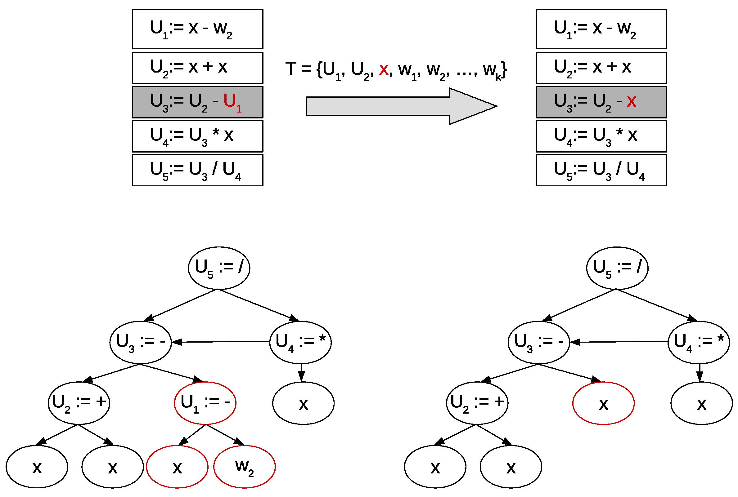
• Mutation operator. Given a SLP table of an individual of the population, a random element of the consequent of a random rule is exchanged for another random symbol. If the selected element is an operator, it is exchanged by another valid operator and if the selected element is an operand, it is exchanged by a terminal symbol or a reference to other rule, as shown in Figure 2. On the other hand, if the mutation operator exchanges a binary operator by an unary operator, the second operand of the rule is left to the value ∅. Nevertheless, if the operator mutes an unary operator to a binary operator, then the second operand is randomly selected from the set of valid operands of the production rule (independent variables, parameters or references to other rules of the SLP table).

Once both single- and multi-objective algorithms have found an algebraic expression, a local search procedure is applied in order to estimate the parameters W for each objective. In this way, both algorithms are able to provide a general algebraic expression which share common behaviour from all datasets (objectives) and parameters are conveniently fitted to satisfy each objective.

4. Experimentation

We tested and experimentally validated both single-objective and multi-objective approaches in two experiment setups:

• A first study attempted to empirically validate whether the described problem can be solved with the proposed formulations. Thus, we built different scenarios with synthetic data, with the aim of validating the performance of each approach under a controlled experimental environment that eases the analysis of performance of the approaches. To that end, Section 4.1 describes a set of benchmark algebraic expressions to be used in the experiments, and the results obtained with each approach. This section ends with a discussion of the results obtained.
• In the second experiment (Section 4.2), we tackled a real problem about energy consumption prediction. In it, we were provided with the energy consumption time series of a set of buildings for which we assumed there is a medium or high correlation and the goal was to find a single parameterised algebraic expression $F(X_i,W_i)$ that can explain the global/common behaviour of all related energy consumption data series.

4.1. Experimentation with Synthetic Data

We used a set of benchmark algebraic expressions to create a set of synthetic datasets with the same ground behaviour. The main goal of this experimentation was to test if the proposal of this paper can be used to obtain a general regression hypothesis that explains all datasets coming from the same algebraic expression, with different parameters W for each dataset, in this controlled environment.

This section is divided into three parts: firstly, Section 4.1.1 explains the set of benchmark algebraic expressions, and how all artificial datasets were generated. Then, Section 4.1.2 and Section 4.1.3 show the experimental configuration used in each approach and the results obtained, respectively.

4.1.1. Data Acquisition

We used six benchmark algebraic expressions (see Equations (4)–(9)) that are widely used in the literature to test the quality of symbolic regression algorithms [52]. More specifically, we selected benchmark algebraic expressions with different complexity (which include polynomial, trigonometrical and exponential expressions) and also with a varying number of parameters (from one parameter (Equations (7)–(9)) to six parameters (Equation (6))). Besides, we generated different datasets for each benchmark algebraic expression to empirically validate if both single-objective and multi-objective approaches have the same behavior, or in contrast, to find which technique carries out a better exploration of the search space when the number of datasets increases.

$$f_1(x_1,x_2)={\displaystyle \frac{e^{-{(x_1-w_1)}^2}}{w_2+{(x_2-w_3)}^2}}$$

(4)

$$f_2(x_1,x_2)={\displaystyle \frac{w_1}{w_1+x_1^{w_2}}}+{\displaystyle \frac{w_1}{w_1+x_2^{w_2}}}$$

(5)

$$f_3(x_1,x_2,x_3,x_4,x_5)=w_1+w_2*{\displaystyle \frac{w_3*x_2+w_4*x_3^2}{w_5*x_4^3+w_6*x_5^4}}$$

(6)

$$f_4(x_1,x_2)=w_1*sin(x_1)*cos(x_2)$$

(7)

$$f_5(x_1,x_2)=(x_1-w_1)*(x_2-w_1)+w_2*sin((x_1-w_3)*(x_2-w_3))$$

(8)

$$f_6(x_1,x_2)=x_1^4-x_1^3+{\displaystyle \frac{x_2}{w_1}}-x_2$$

(9)

We generated five datasets for each benchmark algebraic expression shown in Equations (4)–(9). All five datasets regarding a single algebraic expression share the same values for the input data, i.e., for each independent variable $x_i$ of each benchmark algebraic expression, we generated 200 samples uniformly distributed in the range $[0.0,1.0]$. After that, we selected different values for the parameters $w_i$ of each dataset regarding the same algebraic expression. Each value $w_i$ was randomly generated in the interval $[0.0,5.0]$. Thus, for each benchmark algebraic expression, we were provided with five datasets with the same inputs but different outputs.

As an example, let us consider the dataset generation for the benchmark algebraic expression of Equation (5): firstly, we generated 200 random samples for $x_1$ and $x_2$, which were used as inputs for all datasets. After that, we generated five different values for each parameter $w_i$: $(w_1^1,w_2^1)=(3.23,4.12)$ for the first dataset; $(w_1^2,w_2^2)=(1.09,2.35)$ for the second dataset; and $(w_1^3,w_2^3)=(2.17,0.59)$, $(w_1^4,w_2^4)=(3.0,0.64)$, and $(w_1^5,w_2^5)=(3.83,1.1)$ for the remaining datasets. This allowed us to obtain different datasets with the same inputs but different outputs, and with a high correlation between all datasets, which is a prerequisite of our proposal.

Both single- and multi-objective approaches were tested in two cases: considering a low number of datasets, and considering a larger number of datasets. We performed an experimentation using three of the five datasets generated for each benchmark algebraic expression, and another experimentation using all datasets, with the goal of discovering if the number of datasets has an influence in the performance of the multi-objective approach.

4.1.2. Experimental Settings

For the experimentation, we used 12 mathematical operators (+, -, *, /, sqrt, pow, exp, sin, cos, log, min, and max) to allow symbolic regression to build algebraic expressions with any combination of these operators. We performed a parameter tuning with different values for both single- and multi-objective approaches to find a suitable configuration that allows us to achieve a better exploration of the search space. Thus, we tested different values for SLP size, genetic operators (crossover and mutation), stopping criterion, etc. After that test, the experimental settings that provided the best results in both approaches were: the population size of 180; allowing 15 rules for each SLP; and crossover and mutation probabilities of 90% and 10%, respectively. Finally, the stopping criteria was evaluating 40,000 solutions.

Each dataset was randomly divided into train (70% of data) and test (remaining 30%). The training data were used during the algorithm execution, and the test data were used once the algorithm finished and returned an algebraic expression, so that we could prevent over-fitting and validate the results in previously unseen data. Finally, we ran 30 executions for each scenario (algorithm and problem) with different random seed numbers, in order to carry out a statistical test that helped us determine if there exist significant differences between the results obtained.

4.1.3. Results and Discussion

The results obtained for each approach and dataset (train and test results) are shown in

Table 1. Results of Single and Multi objective approaches in benchmark train and test datasets.

Items	3 Datasets						5 Datasets
	${\mathit{f}}_1$	${\mathit{f}}_2$	${\mathit{f}}_3$	${\mathit{f}}_4$	${\mathit{f}}_5$	${\mathit{f}}_6$	${\mathit{f}}_1$	${\mathit{f}}_2$	${\mathit{f}}_3$	${\mathit{f}}_4$	${\mathit{f}}_5$	${\mathit{f}}_6$
TRAIN
	Single objective
Median	$3.12\times {10}^{-16}$	$1.53\times {10}^{-2}$	$1.89\times {10}^8$	$1.45\times {10}^{-7}$	$4.92$	$4.46\times {10}^{-5}$	$7.81\times {10}^{-10}$	$5.5\times {10}^{-2}$	$3.99\times {10}^7$	$6.27\times {10}^{-6}$	$3.75$	$5.55\times {10}^{-5}$
Best	$6.45\times {10}^{-18}$	$6.2\times {10}^{-4}$	$2.18\times {10}^6$	$1.37\times {10}^{-9}$	$1.2\times {10}^{-1}$	$2.62\times {10}^{-11}$	$2.97\times {10}^{-11}$	$2.1\times {10}^{-3}$	$8.77\times {10}^6$	$2.03\times {10}^{-9}$	$2.1\times {10}^{-1}$	$4.91\times {10}^{-11}$
Worst	$1.52\times {10}^{-14}$	$4.5\times {10}^{-2}$	$4.86\times {10}^8$	$6.61\times {10}^{-3}$	$1.76\times {10}^1$	$1.77\times {10}^{-3}$	$5.67\times {10}^{-8}$	$8.9\times {10}^{-2}$	$9.41\times {10}^7$	$6.33\times {10}^{-3}$	$1.83\times {10}^1$	$3.18\times {10}^{-3}$
Time (s.)	$1.03\times {10}^3$	$1.3\times {10}^3$	$1.81\times {10}^3$	$1.21\times {10}^3$	$1.35\times {10}^3$	$1.17\times {10}^3$	$2.03\times {10}^3$	$2.14\times {10}^3$	$2.14\times {10}^3$	$2.06\times {10}^3$	$2.16\times {10}^3$	$1.96\times {10}^3$
Size	$8.93$	$10.6$	$11.76$	$9.96$	$11.16$	$11.23$	$9.63$	$10.5$	$10.76$	$10.33$	$11.56$	$10.9$
Parameters	$2.8$	$3.33$	$2.83$	$3.2$	$3.16$	$3.33$	$3.13$	$3.3$	$2.66$	$2.83$	$3.36$	$3.2$
	Multi objective
Median	$4.6\times {10}^{-15}$	$3.1\times {10}^{-3}$	$8.49\times {10}^6$	$2.87\times {10}^{-7}$	$9.4\times {10}^{-1}$	$2.12\times {10}^{-6}$	$1.13\times {10}^{-8}$	$8\times {10}^{-2}$	$4.43\times {10}^7$	$5.62\times {10}^{-7}$	$1.75\times {10}^1$	$3.95\times {10}^{-6}$
Best	$3.54\times {10}^{-18}$	$3.83\times {10}^{-5}$	$1.21\times {10}^5$	$1.36\times {10}^{-9}$	$1.09\times {10}^{-1}$	$2.58\times {10}^{-11}$	$2.92\times {10}^{-11}$	$1.2\times {10}^{-3}$	$1.11\times {10}^6$	$2\times {10}^{-9}$	$7.2\times {10}^{-1}$	$4.86\times {10}^{-11}$
Worst	$2.59\times {10}^{-13}$	$4.3\times {10}^{-1}$	$1.32\times {10}^9$	$3.92\times {10}^{-2}$	$3.78\times {10}^2$	$1.19\times {10}^{-3}$	$8.14\times {10}^{-7}$	$2.22$	$2\times {10}^9$	$2.54\times {10}^{-1}$	$3.07\times {10}^2$	$6.88\times {10}^{-3}$
Time (s.)	$1.38\times {10}^3$	$1.91\times {10}^3$	$2.58\times {10}^3$	$1.72\times {10}^3$	$3.12\times {10}^3$	$1.67\times {10}^3$	$2.43\times {10}^3$	$2.89\times {10}^3$	$4.47\times {10}^3$	$2.96\times {10}^3$	$5.49\times {10}^3$	$2.9\times {10}^3$
Size	$11.76$	$12.1$	$12.76$	$12.7$	12	$13.23$	$7.56$	$9.96$	$11.76$	$12.36$	$10.33$	$13.1$
Parameters	3	$3.53$	$2.7$	$3.3$	$3.1$	$3.86$	$2.43$	$3.03$	$2.23$	$3.53$	$3.06$	$3.8$
TEST
	Single-Objective
Median	$2.01\times {10}^{-15}$	$2.42\times {10}^{-2}$	$8.21\times {10}^4$	$8.94\times {10}^{-8}$	$5.52$	$9.63\times {10}^{-5}$	$1.79\times {10}^{-9}$	$4.9\times {10}^{-2}$	$1.09\times {10}^5$	$4.38\times {10}^{-5}$	$3.91$	$3.95\times {10}^{-4}$
Best	$7.94\times {10}^{-18}$	$1.3\times {10}^{-3}$	$2.26\times {10}^4$	$7.19\times {10}^{-10}$	$1.4\times {10}^{-1}$	$2.44\times {10}^{-11}$	$4.21\times {10}^{-11}$	$3.2\times {10}^{-3}$	$3.67\times {10}^4$	$1.19\times {10}^{-9}$	$1.5\times {10}^{-1}$	$4.36\times {10}^{-11}$
Worst	$3.6\times {10}^{-1}$	$6.18$	$1.65\times {10}^5$	$4.7\times {10}^{-2}$	$9.38\times {10}^2$	$1.97$	$1.1\times {10}^{-5}$	$2.4\times {10}^{-1}$	$2.28\times {10}^5$	$1.67\times {10}^{-2}$	$1.23\times {10}^3$	$2.72\times {10}^{-1}$
	Multi-Objective
Median	$1.36\times {10}^{-12}$	$1.05\times {10}^1$	$1.65\times {10}^5$	$5.3$	$9.7\times {10}^2$	$2.6\times {10}^{-1}$	$1.59\times {10}^{-6}$	$1.83\times {10}^1$	$2.28\times {10}^5$	$3.05$	$9.33\times {10}^2$	$6.6\times {10}^{-1}$
Best	$1.36\times {10}^{-12}$	$8.57$	$1.45\times {10}^5$	$1.08$	$4.67\times {10}^2$	$6\times {10}^{-2}$	$1.32\times {10}^{-6}$	$1.23\times {10}^1$	$1.97\times {10}^5$	$1.65$	$8.1\times {10}^2$	$7\times {10}^{-2}$
Worst	3	$4.22\times {10}^1$	$1.66\times {10}^5$	$5.3$	$1.08\times {10}^3$	$1.52\times {10}^1$	$1.58\times {10}^{-6}$	$8.6\times {10}^1$	$2.29\times {10}^5$	$7.51$	$1.28\times {10}^3$	$6.7\times {10}^{-1}$

. The first column of this table describes the item evaluated for each approach, i.e., Median, Best (lowest), and Worst (highest) Mean Square Error (MSE), the average execution time of each approach (item Time (s.)), the average size of the resulting algebraic expression found by the algorithms (item Size), and the average number of parameters used by the resulting algebraic expressions (item Parameters). We highlight that we used the median error as statistical analysis estimator since the resulting MSE error distributions of the algorithms do not follow a normal distribution. In these cases, the mean error cannot be considered an appropriate metric, and it is replaced by the median value.

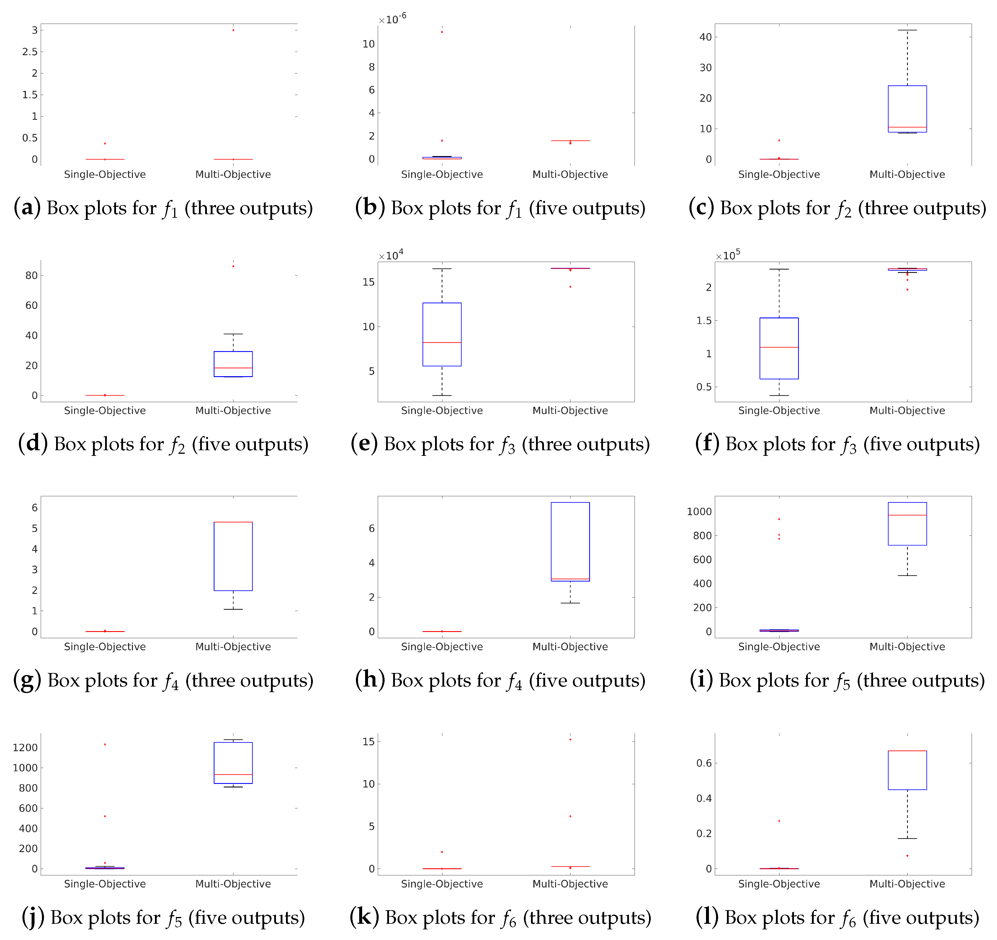
Columns 2–7 contain the results provided by both single- and multi-objective approaches for each benchmark algebraic expression ($f_1$–$f_6$) that was used to generate three datasets, and Columns 8–13 gather the results after modelling five datasets generated with each benchmark algebraic expression. Finally, Rows 3–17 describe the results in train data, whereas Rows 18–26 gather the results in test data. To give support to the analysis, we also provide box plots about the MSE distributions in the test sets for each single- and multi-objective approach (see Figure 3).

In a preliminary analysis of the test results in Table 1 and Figure 3, we observed that the single-objective approach achieved the lowest median MSE in five of six problems with three datasets, and all problems with five datasets. In addition, the best solution found was provided by the single-objective approach in both cases. Finally, the worst MSE also suggests that the single-objective algorithm performed better in all problems with three datasets, and in five of six problems with five datasets. After this preliminary analysis, we validated this assumption statistically, using a non-parametric Kruskal–Wallis (KW) test with 95% confidence level to verify whether significant differences exist between the results found with each algorithm.

Table 2. Statistical tests to compare algorithms in the results of all benchmark algebraic expressions.

	Train		Test
	3 Datasets	5 Datasets	3 Datasets	5 Datasets
$f_1$	$1.7\times {10}^{-1}$ (x)	$4.9\times {10}^{-3}$ (+)	$2.87\times {10}^{-9}$ (+)	$1.39\times {10}^{-10}$ (+)
$f_2$	$1.3\times {10}^{-1}$ (x)	$2.8\times {10}^{-2}$ (+)	$2.83\times {10}^{-11}$ (+)	$2.86\times {10}^{-11}$ (+)
$f_3$	$1.4\times {10}^{-2}$ (-)	$7.9\times {10}^{-1}$ (x)	$3.95\times {10}^{-11}$ (+)	$1.22\times {10}^{-10}$ (+)
$f_4$	$8.01\times {10}^{-1}$ (x)	$8.01\times {10}^{-1}$ (x)	$1.67\times {10}^{-11}$ (+)	$2.62\times {10}^{-11}$ (+)
$f_5$	$5.8\times {10}^{-1}$ (x)	$2.8\times {10}^{-4}$ (+)	$2.79\times {10}^{-10}$ (+)	$2.41\times {10}^{-11}$ (+)
$f_6$	$7\times {10}^{-3}$ (-)	$1.9\times {10}^{-1}$ (x)	$7.55\times {10}^{-11}$ (+)	$1.81\times {10}^{-11}$ (+)

summarises the results of the test, and it contains the resulting p-value of the test for both training (Columns 2 and 3) and test data (Columns 4 and 5). If significant differences were found between the results found with the single- and multi-objective approaches (p-value $<0.05$), then the results were marked: with “+” if the single-objective approach found a better solution; with “-” if the multi-objective algorithm was better; and with “x” if there were no significant differences between the solutions.

As shown in Table 2, our preliminary analysis was confirmed by results in Columns 4 and 5, since the single-objective approach improved significantly the multi-objective algorithm in all cases. After the statistical test was applied over the training error distributions, Table 2 confirms that the multi-objective approach was better in two of six problems with three datasets than the single-objective approach, considering training results; and there were no statistical differences in the remaining four problems. Regarding the problems with five datasets, the multi-objective approach was equivalent to the single-objective approach in three problems also considering training results, and the single-objective algorithm was better in the remaining three. On the other hand, the results provided in Table 1 as well as the statistical test results in Table 2 suggest that the single-objective algorithm improves performance over the multi-objective approach in the test data. This fact suggests that the multi-objective approach might be over-fitting the training data, therefore providing worse results in the test sets of each problem than the single-objective approach. This assumption is supported by the size of the resulting algebraic expressions, provided in Table 1. The single-objective algorithm could provide simpler (shorter) expressions, while the multi-objective approach provided more complex expressions that could overfit training data and could not generalise well to all datasets. This also affected the training time of each method. As the multi-objective algorithm considered larger expressions, its evaluation was computationally more expensive than the single-objective algorithm (see item Time (s.) in Table 1).

To conclude the analysis of results in this section, we note that the single-objective approach could find better solutions than the multi-objective approach in terms of generalisation, without any regards to the number of datasets for each problem. In this way, the multi-objective approach overfit the training data, especially when the number of objectives (datasets) was low.

4.2. Experimentation with Real Data

With the approaches validated under a controlled environment, this section describes the testing with real data. As problem statement, we were provided with a set of energy consumption time series of different buildings (one time series $x_i$ for each building i), together with an additional time series of exogenous data with the ambient temperature T. We name the energy consumption of a building i at time instant t as $x_i(t)$, and the temperature at time instant t as $T(t)$. All buildings are located in the same area, so that the temperature time series is the same for all buildings.

Our goal was to find a single algebraic expression f such as $x_i(t+1)=f(x_i(t),x_i(t-1),\cdots ,x_i(t-h)$, $T(t+1),T(t),\cdots ,T(t-h+1),w_i)$, which can provide us with an approximation of the next energy consumption value of any building, $x_i(t+1)$, considering previous values of the same energy consumption time series up to a time horizon h, and the h previous values of the temperature. The resulting algebraic expression that models the energy consumption time series must be the same for all buildings, except for the parameters $W_i$, which are different for each building.

This could be possible only if the data series of all buildings are not independent and there exists a relationship among them. For this reason, it was important to check as prerequisite that the correlation coefficient of all time series in a dataset is medium or high, as a measurement of dependency (not necessarily causality) between all time series. If this hypothesis were confirmed, then the proposed methods would be expected to find a generalisation of that behavior in terms of a parameterised general algebraic expression able to predict the energy consumption of each building.

4.2.1. Data Acquisition

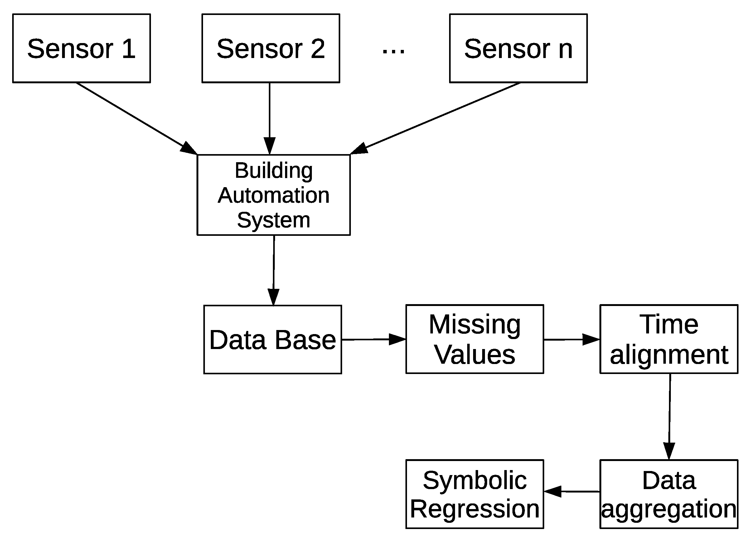
We used a dataset that contains the energy consumption of seven different buildings of University of Granada (south of Spain) from March 2013 to October 2015, named from $B_1$ to $B_7$ for confidentiality reasons. Each building is equipped with a set of sensors that monitor their energy consumption (kW/h) hourly. A Building Automation System (BAS) is responsible to monitor the energy consumption measured for each sensor of each building and store all data in a database.

The raw data stored in the database needed to be preprocessed because there could be missing data due to light cuts, sensor failures, etc. The data preprocessing process used in this experimentation is shown in Figure 4. The first step of this preprocessing stage consisted in seeking missing values and interpolating each of them (which are 5% of the data). After that, a time alignment was necessary to obtain the data consumption in the same temporal range. Besides, since this experiment attempted to predict the energy consumption of different buildings using the data of previous days, it was necessary to calculate the energy consumption for each weekday as the aggregation (addition) of the kW consumed in 24 h of the same day. Finally, to work with uniform data, we normalised the data in the interval $[0.0,1.0]$ (see Equation (10), where $v_i$ is the response value, $v_{min}$ is the minimum response observed, $v_{max}$ is the maximum response observed and $r_{normalised}$ is the normalised response value). Once all data were preprocessed, we transformed the univariate dataset into a multivariate dataset, with eight dimensions, each one for a weekday plus the weekly temperature.

$$r_{normalized}={\displaystyle \frac{v_i-v_{min}}{v_{max}-v_{min}}}$$

(10)

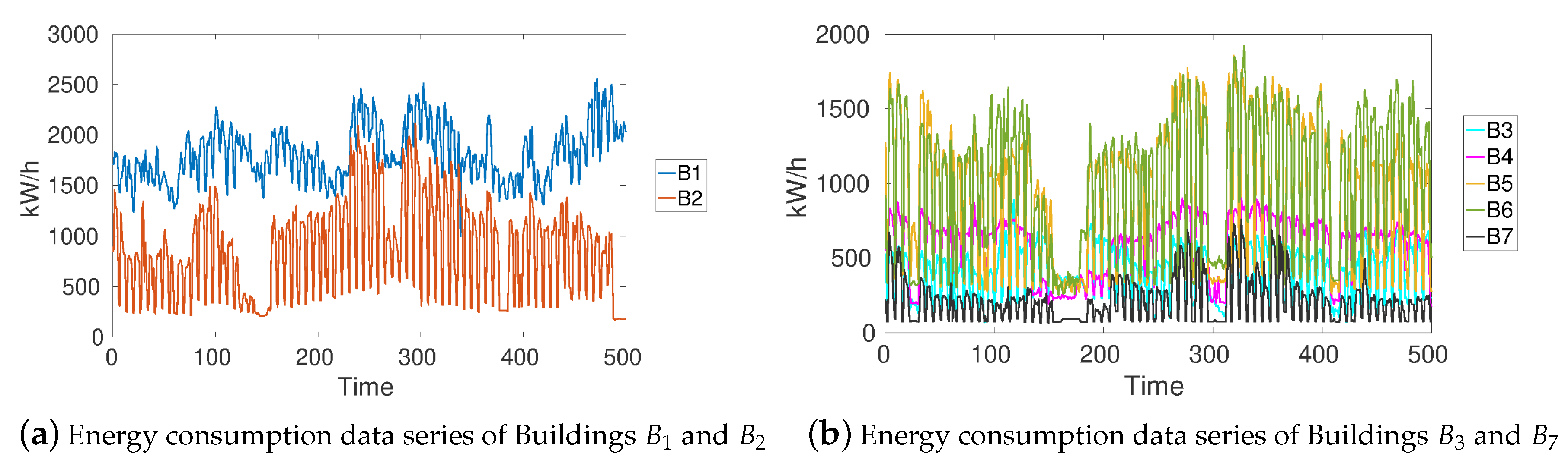
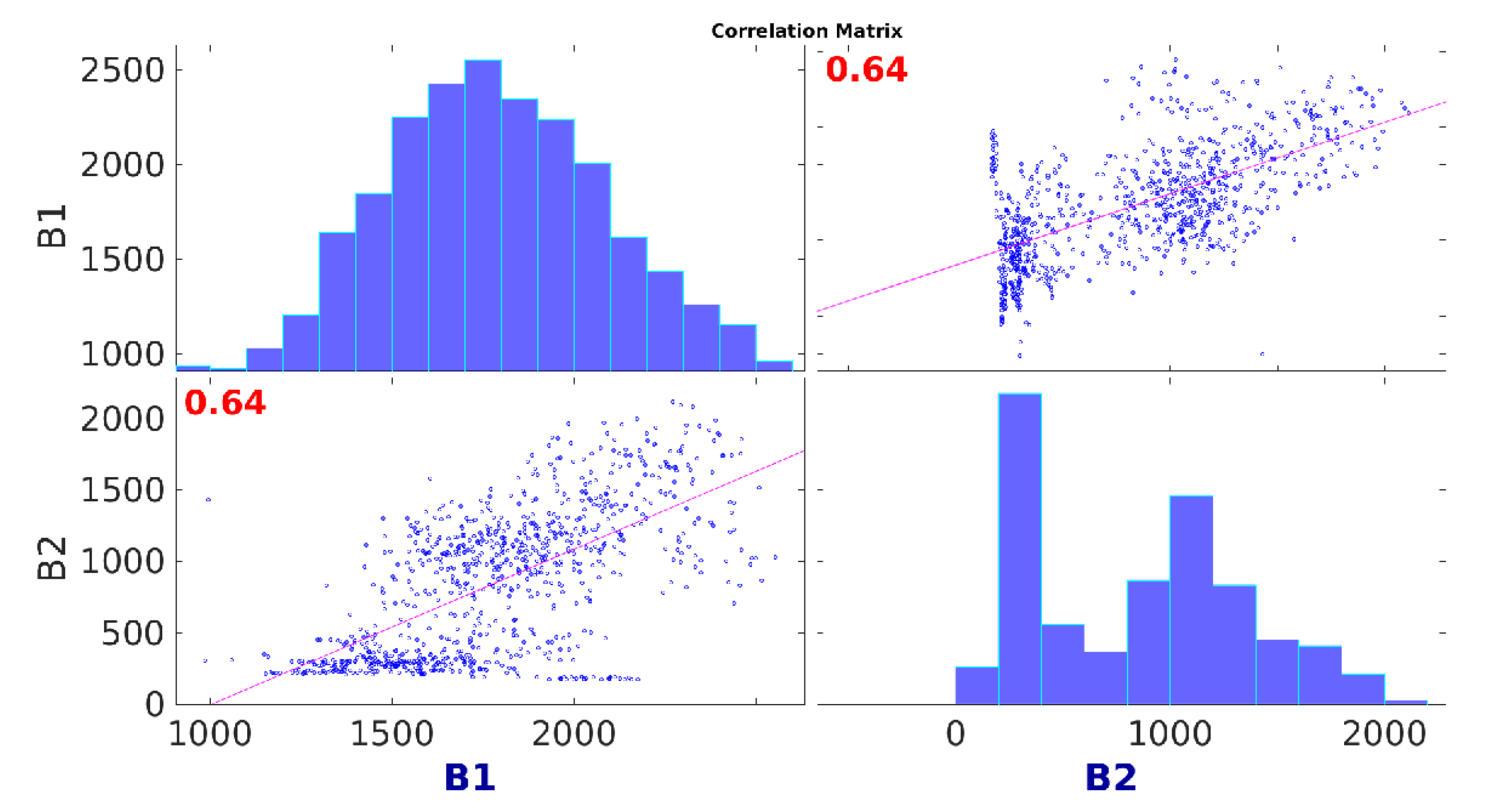
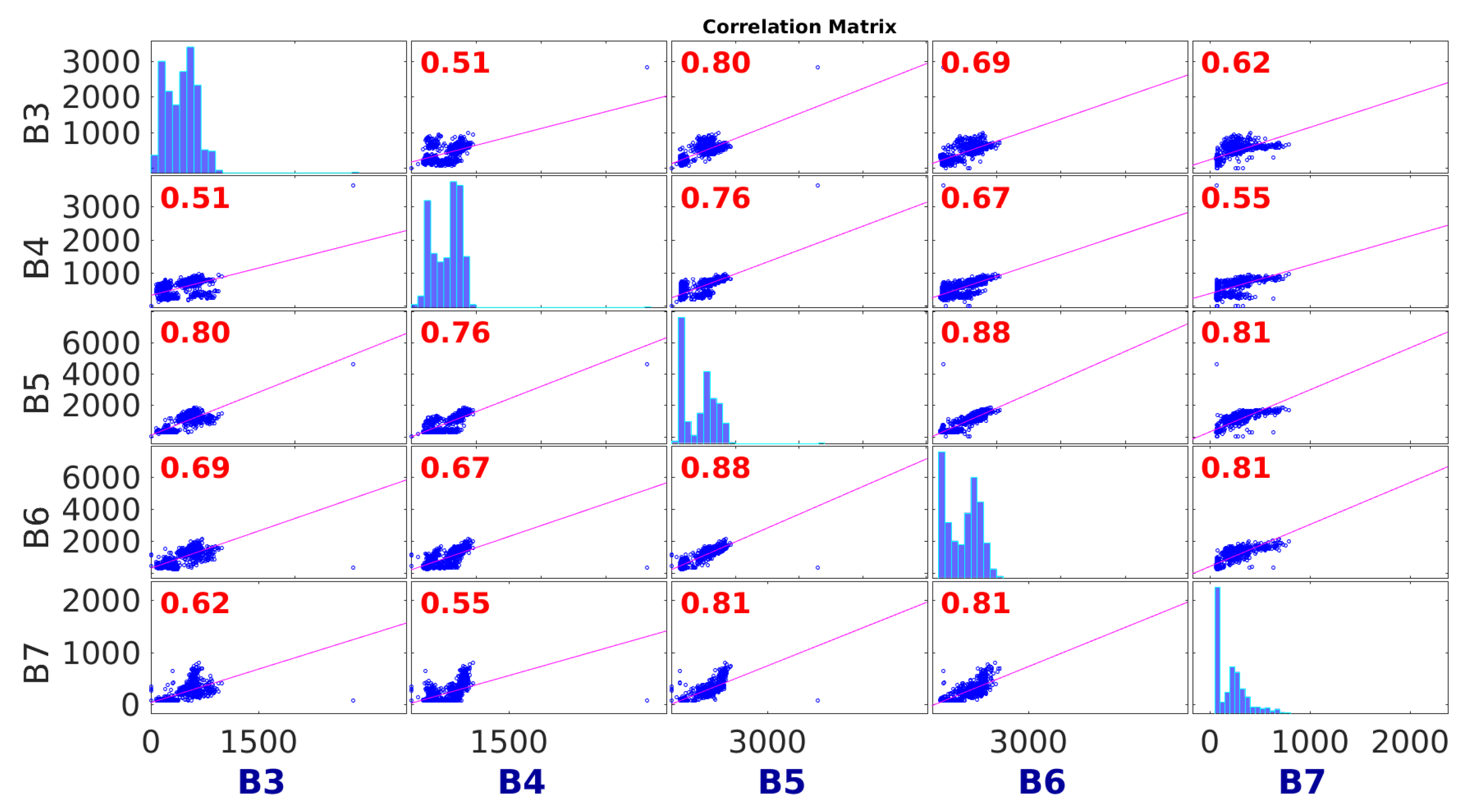
Once all data were preprocessed, it was necessary to carry out a preliminary correlation study between the energy consumption of all buildings to know if energy consumption data series are medium or highly correlated as the initial hypothesis to apply the proposed models. As the labels low, medium or high correlation levels are subjective and problem dependent, in our research, we considered low correlations with values less than $0.3$, whereas correlation values between $0.3$ and $0.7$ were considered to medium correlation and values higher than 0.7 were considered highly correlated. As a result of this study, we found two clusters with medium or high correlation coefficients. Buildings $B_1$ and $B_2$ formed a cluster, and the second cluster was composed of Buildings $B_3$–$B_7$. An example of the energy consumption data series of each set of buildings is shown in Figure 5.

Figure 6 and Figure 7 show the correlation plot matrices of the energy consumption time series for each building. The diagonal of the plot matrices gathers the histogram, to know how the energy consumption is distributed in each building. Then, the remaining subfigures show the scatter plot between the energy consumption of each pair of buildings. A subfigure in a cell (i,j) shows the relationships between building at row i (y-axis) and the building at column j (x-axis), plus the correlation coefficient R highlighted in red, whose values are in the interval $[-1.0,1.0]$. Values of R closer to $1.0$ mean a positive correlation, whereas values near to $-1.0$ suggest negative correlation. Finally, values closer to $0.0$ suggest low correlation.

As shown in Figure 6 and Figure 7, there are medium ($0.3<R<0.7$) and high ($R>0.7$) positive correlations between the energy consumption of the selected buildings in each cluster. Thus, we were provided with two different scenarios to test our approaches: One being composed of two datasets with Buildings $B_1$ and $B_2$ and another one with five datasets with Buildings $B_3$–$B_7$. To ease the explanation in the experimental section, we named each cluster of buildings as $E_1$ (for Buildings $B_1$ and $B_2$) and $E_2$ (for Buildings $B_3$–$B_7$).

In the experiments, we divided each dataset into two subsets: training (70%) and test (30%), to avoid over-fitting in the solutions found. In this way, the training set was used to build the model of each approach and the test set was used to check the quality of the solutions found, following the same methodology presented in Section 4.1. Therefore, to verify the robustness of each approach, we show in Section 4.2.3 the results obtained in each training and test subsets.

4.2.2. Experimental Settings

To define the experimental settings of each approach used in a real scenario with energy consumption data, we performed a trial-and-error procedure to find the optimal parameters for the algorithm. As is described, we allowed a maximum size of 15 operations (SLP size), which can use a set of 12 mathematical operators (+, -, *, /, $sqrt,pow,exp,sin,cos,log,min$, and max). Thus, as mentioned above, the input variables for each approach were composed of the energy consumption registered in the previous h weekdays ($h=6$ for this experimentation) and the temperature registered for the last weekday. In addition, we permitted a set of five parameters $W_i=(w_i^1,w_i^2,w_i^3,w_i^4,w_i^5)$ for each building, which were estimated for each building during the algorithm execution. Then, the crossover and mutation probabilities were established as 90% and 10%, respectively. Finally, both approaches ran 30 times with different random seeds to analyse the results statistically. The stopping criteria used for each algorithm was to have 40,000 solutions evaluated.

4.2.3. Results and Discussion

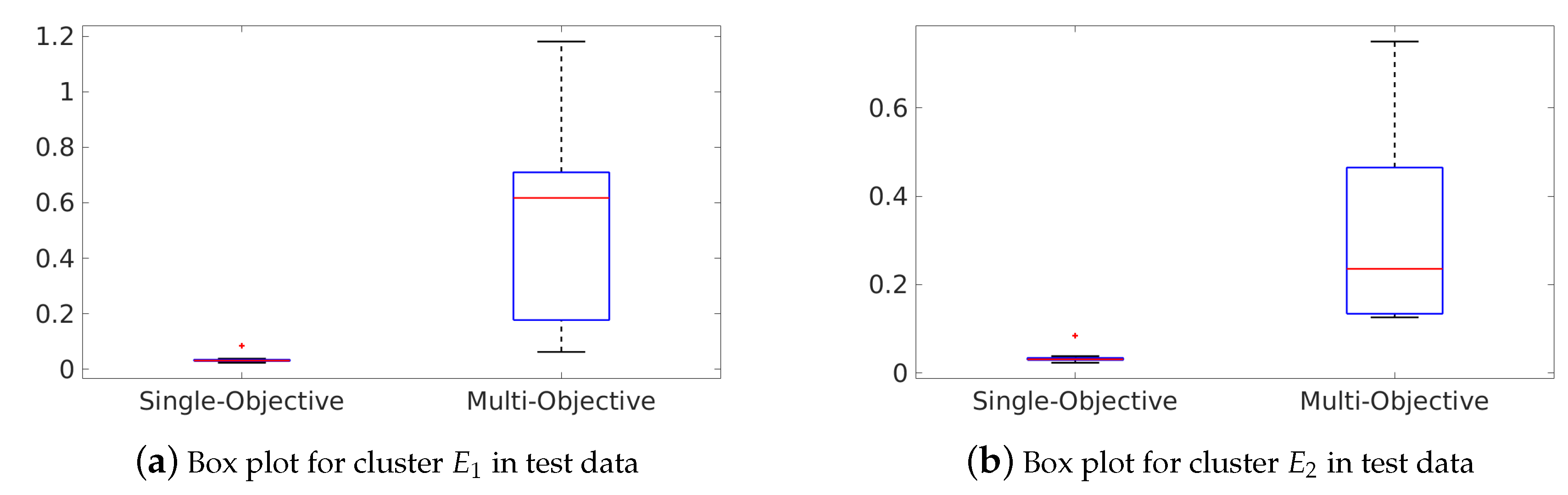
The results of this experimentation are organised in

Table 3. Results for cluster of buildings $E_1$ and $E_2$ in train and test data.

	Train		Test
	${\mathit{E}}_1$	${\mathit{E}}_2$	${\mathit{E}}_1$	${\mathit{E}}_2$
	Single-Objective
Median	$2.3\times {10}^{-2}$	$6.7\times {10}^{-2}$	$3.1\times {10}^{-2}$	$7.2\times {10}^{-2}$
Best	$1.6\times {10}^{-2}$	$5.5\times {10}^{-2}$	$2.3\times {10}^{-2}$	$5.3\times {10}^{-2}$
Worst	$3\times {10}^{-2}$	$8.1\times {10}^{-2}$	$8.4\times {10}^{-2}$	$2.4\times {10}^{-1}$
Time	$1.02\times {10}^3$	$2.53\times {10}^3$	-	-
Size	10.83	11.56	-	-
Parameters	2.43	3	-	-
	Multi-Objective
Median	$1.9\times {10}^{-2}$	$6.8\times {10}^{-2}$	$3.1\times {10}^{-2}$	$7.2\times {10}^{-2}$
Best	$1.4\times {10}^{-2}$	$5.1\times {10}^{-2}$	$2.3\times {10}^{-2}$	$5.3\times {10}^{-2}$
Worst	$3.7\times {10}^{-2}$	$1.1\times {10}^{-1}$	$8.4\times {10}^{-2}$	$2.4\times {10}^{-1}$
Time	$1.61\times {10}^3$	$4.12\times {10}^3$	-	-
Size	11.03	4.73	-	-
Parameters	2.9	1.46	-	-
KW Test	$4.49\times {10}^{-5}$ (-)	$0.35$ (x)	$2.9\times {10}^{-11}$ (+)	$1.21\times {10}^{-10}$ (+)

. In this table, Column 1 shows the item evaluated for each single- and multi-objective approach. Thus, rows labeled as Median describe the median Mean Square Error (MSE) obtained in the 30 experiments for both approaches. Rows named as Best and Worst gather the minimum and maximum MSE obtained in the 30 runnings. Then, the average time needed to obtain a solution by each approach is shown in rows labeled as Time (s.). Rows labeled as Size encode the average size of each algebraic expression found in each run (calculated as the number of mathematical operators used in the algebraic expression found), and the number of parameters used in the algebraic expression found with each single- and multi-objective approach are also shown in rows tagged as Parameters. Finally, Columns 2 and 3 of the table gather the results obtained by both single- and multi-objective approach for each cluster of buildings ($E_1$ and $E_2$), respectively, in training data and Columns 3 and 4 show the results obtained by both single- and multi-objective approach in test data. Finally, last row of Table 3 describes the results of Kruskal–Wallis test. To provide a better analysis of the results of Table 3 we have also included the box plots of the MSE distributions in the test sets for both single- and multi-objective approach in Figure 8.

In a first analysis of the results of both single- and multi-objective approach in test data in Table 3, we may observe that the single-objective approach obtained the lowest MSE median value in both clusters of buildings. Moreover, since the single-objective approach provided the best solution in terms of best MSE in both scenarios and the multi-objective approach found the worst solution in both sets of buildings $E_1$ and $E_2$, this preliminary analysis suggests that the single-objective approach is potentially better than the multi-objective approach.

To give support of this analysis, we again performed a non-parametric Kruskal–Wallis test (KW) with a 95% confidence level to statistically validate if there are significant differences between each approach. The results of the KW test are presented in the last row of Table 3, where Columns 2–3 and 4–5 show the resulting p-value of the KW test for each cluster of buildings and approaches for both training and test datasets. If significant differences were found between the results obtained with the single- and multi-objective approach (p-value $<0.05$), then the results were marked with the symbol + if the single-objective approach was better; with the symbol - if the multi-objective approach provided better solutions; and with the symbol x if both approaches were equivalents.

Regarding the results of the KW test in Table 3 in test data (Columns 4 and 5), the single-objective approach provided better results than the multi-objective approach in all cases, thus confirming our hypothesis that the single-objective is better than the multi-objective approach in test data. Box plots in Figure 8 visually confirm that there are significant differences between the results found by the multi-objective approach in the problems of buildings in $E_1$ and buildings in $E_2$, respectively. Nevertheless, regarding the results of the KW test in train data (Columns 2 and 3 of the last row of Table 3), we may observe that the multi-objective approach provided better solutions for $E_1$ (two objectives), and no significant differences between the single- and multi-objective approach were found in $E_2$ (five objectives).

If we analyse the results of each approach in train data in Table 3 regarding the median and best MSE value, the multi-objective approach provided the lowest value in the cluster of buildings $E_1$, and the single-objective approach achieved better results in the second cluster of buildings $E_2$. Nevertheless, in both scenarios, the multi-objective approach performed worse in terms of MSE value. This fact, together with the results of the KW test, suggests that the multi-objective approach suffered over-fitting in the training procedure, and therefore it shows the same performance we found in synthetic datasets in Section 4.1. Therefore, as an example of the solutions found by both approaches in real energy consumption data, Equations (11) and (12) gather the best SLP found by each single- and multi-objective approach, respectively. We also want to remark that, although we allowed SLPs with size equal to 15, the equations shown are the useful code for each SLP. Then, the algebraic expression encoded by each SLP can be calculated by generating the last rule of each equation. Finally, regarding the average algebraic expression size shown in Table 3, we cannot conclude that there are significant differences between both single- and multi-objective approaches, since the multi-objective approach found smaller solutions for $E_2$, whereas the single-objective approach provided smaller solutions in the first cluster of buildings $E_1$. Nevertheless, regarding the computational time, the multi-objective approach was considerably higher than the single-objective approach in both cases, which may be a consequence of the Pareto-optimal solution search in multi-objective algorithms that need more computational time, as argued in Section 2.

$$E_1\left\{\begin{array}{c}{U}_6\to min(w_4,x_1)\hfill \\ U_7\to x_5/U_6\hfill \\ U_8\to w_2+U_7\hfill \\ U_9\to max(x_6,U_8)\hfill \\ U_{10}\to pow(U_9,x_2)\hfill \\ U_{11}\to w_2+U_{10}\hfill \\ U_{12}\to max(x_6,U_{11})\hfill \\ U_{13}\to w_2+U_{12}\hfill \\ U_{14}\to pow(x_6,U_{13})\hfill \\ U_{15}\to w_2+U_{14}\hfill \end{array}\right.E_2\left\{\begin{array}{c}{U}_2\to exp(w_2)\hfill \\ U_3\to x_6-x_1\hfill \\ U_4\to pow(U_2,U_3)\hfill \\ U_5\to cos(x_1)\hfill \\ U_6\to pow(U_4,U_5)\hfill \\ U_7\to w_4*U_6\hfill \\ U_8\to w_4*U_7\hfill \\ U_9\to w_3+x_5\hfill \\ U_{10}\to U_8*U_9\hfill \\ U_{11}\to U_{10}-x_5\hfill \\ U_{12}\to x_4+x_2\hfill \\ U_{13}\to pow(U_{11},U_{12})\hfill \\ U_{14}\to pow(x_6,U_{13})\hfill \\ U_{15}\to U_{14}*w_1\hfill \end{array}\right.$$

(11)

$$E_1\left\{\begin{array}{c}{U}_1\to w_3+x_4\hfill \\ U_8\to exp(U_1)\hfill \end{array}\right.E_2\left\{\begin{array}{c}{U}_2\to tan(x_1)\hfill \end{array}\right.$$

(12)

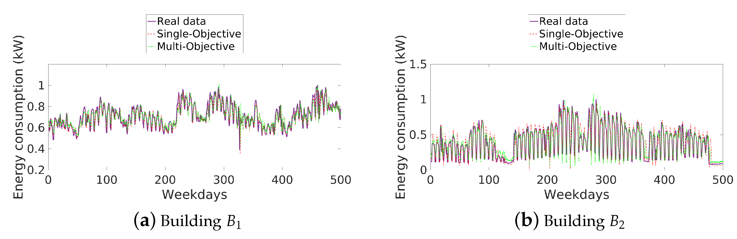
To conclude with the analysis of the results, Figure 9 and Figure 10 show in colour purple the original dataset of the cluster of buildings $E_1$ (Buildings $B_1$ and $B_2$) and $E_2$ (Buildings $B_3$–$B_7$), and the results of the predicted data from both single- and multi-objective approaches in red and green colours, respectively. The results plotted with each approach were obtained with the best algebraic expression found from each approach (see Equations (11) and (12)). In this way, we may conclude that not only was the single-objective approach able to find better solutions than the multi-objective approach in terms of generalisation, without regards the number of datasets for each problem, but also that the provided algebraic expression is an accurate model of energy consumption for all buildings in the same compound $E_1$ or $E_2$.

As a general summary of this experimental section, we may conclude that the approach in this manuscript is able to find a generalised regression hypothesis able to explain multiple datasets. More specifically, when applied to real energy consumption data series, the proposal could find a general explanation about how energy consumption evolves in different buildings, and to provide a single formula that is valid to explain the energy consumption behaviour of all buildings.

5. Conclusions

This work describes our new formulation of energy consumption forecasting in the case where multiple energy consumption time series are under study. To use such approach, we require that all the input time series have a medium or high correlation and, consequently, that a common ground behaviour that can explain (at least partially) all time series exists. As we have not found any other approach in the literature that addresses this particular problem, we developed an experimentation to test the approach under a controlled environment in the laboratory, and then using real data. According to the experimental results, we can confirm that the results in both synthetic and real data are consistent, and that the single-objective algorithm proposed is the best option to find such algebraic expression. Besides, we observed that the performance of Pareto-based multi-objective algorithms decreases as the number of objectives increases, since both experiments showed that the multi-objective algorithm was significantly worse than the single-objective approach when the number of datasets was high. A final observation is that there were significant differences between the error distribution in training and test datasets, which suggest us that the multi-objective approach may over-fit the training data.

In summary, we have provided the scientific community with a new tool to analyse and generalise multiple datasets, and to perform data mining over energy consumption modelling problems. Thus, the proposed model opens new opportunities not only in energy consumption forecasting, but also in other topics such as time series data summarisation, energy profile mining, and anomaly detection. Future works attempt to apply ontologies not only to automatically select the most affordable Pareto-solution regarding semantic knowledge, but also to reduce the search space including knowledge about algebraic expressions.

References

- Santamouris, M. Innovating to zero the building sector in Europe: Minimising the energy consumption, eradication of the energy poverty and mitigating the local climate change. Sol. Energy 2016, 128, 61–94. [Google Scholar] [CrossRef]
- Berardi, U. A cross-country comparison of the building energy consumptions and their trends. Resour. Conserv. Recycl. 2017, 123, 230–241. [Google Scholar] [CrossRef]
- Höller, J.; Tsiatsis, V.; Mulligan, C.; Karnouskos, S.; Avesand, S.; Boyle, D. Chapter 13—Commercial Building Automation. In From Machine-To-Machine to the Internet of Things; Academic Press: Cambridge, MA, USA, 2014; pp. 269–279. [Google Scholar]
- Molina-Solana, M.; Ruiz, M.M.R.D.; Gómez-Romero, J.; Martin-Bautista, M. Data Science for Building Energy Management: A review. Renew. Sustain. Energy Rev. 2017, 70, 598–609. [Google Scholar] [CrossRef]
- Chou, J.S.; Telaga, A.S. Real-time detection of anomalous power consumption. Renew. Sustain. Energy Rev. 2014, 33, 400–411. [Google Scholar] [CrossRef]
- Cui, W.; Wang, H. A New Anomaly Detection System for School Electricity Consumption Data. Information 2017, 8, 151. [Google Scholar] [CrossRef]
- Lü, X.; Lu, T.; Kibert, C.J.; Viljanen, M. Modeling and forecasting energy consumption for heterogeneous buildings using a physical–statistical approach. Appl. Energy 2015, 144, 261–275. [Google Scholar] [CrossRef]
- Gourlis, G.; Kovacic, I. Building Information Modelling for analysis of energy efficient industrial buildings—A case study. Renew. Sustain. Energy Rev. 2017, 68, 953–963. [Google Scholar] [CrossRef]
- Guan, J.; Nord, N.; Chen, S. Energy planning of university campus building complex: Energy usage and coincidental analysis of individual buildings with a case study. Energy Build. 2016, 124, 99–111. [Google Scholar] [CrossRef] [Green Version]
- Gomez, J.A.; Anjos, M.F. Power capacity profile estimation for building heating and cooling in demand-side management. Appl. Energy 2017, 191, 492–501. [Google Scholar] [CrossRef]
- Capozzoli, A.; Piscitelli, M.S.; Brandi, S. Mining typical load profiles in buildings to support energy management in the smart city context. Energy Procedia 2017, 134, 865–874. [Google Scholar] [CrossRef]
- Zhao, J.; Lasternas, B.; Lam, K.P.; Yun, R.; Loftness, V. Occupant behavior and schedule modeling for building energy simulation through office appliance power consumption data mining. Energy Build. 2014, 82, 341–355. [Google Scholar] [CrossRef]
- Balaji, B.; Xu, J.; Nwokafor, A.; Gupta, R.; Agarwal, Y. Sentinel: Occupancy Based HVAC Actuation Using Existing WiFi Infrastructure Within Commercial Buildings. In Proceedings of the 11th ACM Conference on Embedded Networked Sensor Systems, Roma, Italy, 11–15 November 2013; pp. 17:1–17:4. [Google Scholar]
- Amber, K.P.; Aslam, M.W.; Mahmood, A.; Kousar, A.; Younis, M.Y.; Akbar, B.; Chaudhary, G.Q.; Hussain, S.K. Energy Consumption Forecasting for University Sector Buildings. Energies 2017, 10, 1579. [Google Scholar] [CrossRef]
- Shabani, A.; Zavalani, O. Hourly Prediction of Building Energy Consumption: An Incremental ANN Approach. Eur. J. Eng. Res. Sci. 2017, 2, 27. [Google Scholar] [CrossRef] [Green Version]
- Neto, A.H.; Fiorelli, F.A.S. Comparison between detailed model simulation and artificial neural network for forecasting building energy consumption. Energy Build. 2008, 40, 2169–2176. [Google Scholar] [CrossRef]
- Biswas, M.R.; Robinson, M.D.; Fumo, N. Prediction of residential building energy consumption: A neural network approach. Energy 2016, 117, 84–92. [Google Scholar] [CrossRef]
- Jain, R.K.; Smith, K.M.; Culligan, P.J.; Taylor, J.E. Forecasting energy consumption of multi-family residential buildings using support vector regression: Investigating the impact of temporal and spatial monitoring granularity on performance accuracy. Appl. Energy 2014, 123, 168–178. [Google Scholar] [CrossRef]
- Deb, C.; Zhang, F.; Yang, J.; Lee, S.E.; Shah, K.W. A review on time series forecasting techniques for building energy consumption. Renew. Sustain. Energy Rev. 2017, 74, 902–924. [Google Scholar] [CrossRef]
- Yasmeen, F.; Sharif, M. Forecasting electricity consumption for Pakistan. Int. J. Emergy Technol. Adv. Eng. 2014, 4, 496–503. [Google Scholar]
- Baca Ruiz, L.G.; Cuéllar, M.P.; Calvo-Flores, M.D.; Jiménez, M.C.P. An Application of Non-Linear Autoregressive Neural Networks to Predict Energy Consumption in Public Buildings. Energies 2016, 9, 684. [Google Scholar] [CrossRef]
- Afram, A.; Janabi-Sharifi, F.; Fung, A.S.; Raahemifar, K. Artificial neural network (ANN) based model predictive control (MPC) and optimization of HVAC systems: A state of the art review and case study of a residential HVAC system. Energy Build. 2017, 141, 96–113. [Google Scholar] [CrossRef]
- Jovanovic, R.Z.; Sretenovic, A.A.; Zivkovic, B.D. Ensemble of various neural networks for prediction of heating energy consumption. Energy Build. 2015, 94, 189–199. [Google Scholar] [CrossRef]
- Ahmad, M.W.; Mourshed, M.; Rezgui, Y. Trees vs Neurons: Comparison between random forest and ANN for high-resolution prediction of building energy consumption. Energy Build. 2017, 147, 77–89. [Google Scholar] [CrossRef]
- Wang, Z.; Srinivasan, R.S. A review of artificial intelligence based building energy use prediction: Contrasting the capabilities of single and ensemble prediction models. Renew. Sustain. Energy Rev. 2017, 75, 796–808. [Google Scholar] [CrossRef]
- Yildiz, B.; Bilbao, J.; Sproul, A. A review and analysis of regression and machine learning models on commercial building electricity load forecasting. Renew. Sustain. Energy Rev. 2017, 73, 1104–1122. [Google Scholar] [CrossRef]
- Braun, M.; Altan, H.; Beck, S. Using regression analysis to predict the future energy consumption of a supermarket in the UK. Appl. Energy 2014, 130, 305–313. [Google Scholar] [CrossRef] [Green Version]
- McKay, B.; Willis, M.J.; Barton, G.W. Using a tree structured genetic algorithm to perform symbolic regression. In Proceedings of the First International Conference on Genetic Algorithms in Engineering Systems: Innovations and Applications, Sheffield, UK, 12–14 September 1995; pp. 487–492. [Google Scholar]
- Willis, M.; Hiden, H.; Marenbach, P.; McKay, B.; Montague, G. Genetic programming: An introduction and survey of applications. In Proceedings of the Second International Conference On Genetic Algorithms in Engineering Systems: Innovations And Applications, Glasgow, UK, 2–4 September 1997; pp. 314–319. [Google Scholar]
- Langdon, W.B. Genetic Programming—Computers Using “Natural Selection” to Generate Programs. In Genetic Programming and Data Structures: Genetic Programming + Data Structures = Automatic Programming! Springer: Boston, MA, USA, 1998; pp. 9–42. [Google Scholar]
- Koza, J.R. Genetic programming as a means for programming computers by natural selection. Stat. Comput. 1994, 4, 87–112. [Google Scholar] [CrossRef]
- Rueda Delgado, R.; Baca Ruíz, L.G.; Pegalajar Cuéllar, M.; Delgado Calvo-Flores, M.; Pegalajar Jiménez, M.D.C. A Comparison Between NARX Neural Networks and Symbolic Regression: An Application for Energy Consumption Forecasting. In Information Processing and Management of Uncertainty in Knowledge-Based Systems. Applications; Springer: Cham, Switzerland, 2018; pp. 16–27. [Google Scholar]
- Yang, G.; Li, W.; Wang, J.; Zhang, D. A comparative study on the influential factors of China’s provincial energy intensity. Energy Policy 2016, 88, 74–85. [Google Scholar] [CrossRef]
- Bhattacharya, M.; Abraham, A.; Nath, B. A Linear Genetic Programming Approach for Modelling Electricity Demand Prediction in Victoria. In Hybrid Information Systems; Abraham, A., Köppen, M., Eds.; Physica-Verlag HD: Heidelberg, Germany, 2002; pp. 379–393. [Google Scholar] [Green Version]
- Behera, R.; Pati, B.B.; Panigrahi, B.P.; Misra, S. An Application of Genetic Programming for Power System Planning and Operation. Int. J. Control Syst. Instrum. 2012, 3, 15–20. [Google Scholar]
- Hassan, G.N.A. Multiobjective Genetic Programming for Financial Portfolio Management in Dynamic Environments. Ph.D. Thesis, University College London, London, UK, 2010. [Google Scholar]
- Marler, R.T.; Arora, J.S. The weighted sum method for multi-objective optimization: New insights. Struct. Multidiscip. Optim. 2010, 41, 853–862. [Google Scholar] [CrossRef]
- Jakob, W.; Gorges-Schleuter, M.; Blume, C. Application of Genetic Algorithms to Task Planning and Learning. In Proceedings of the Parallel Problem Solving from Nature 2, PPSN-II, Brussels, Belgium, 28–30 September 1992; pp. 293–302. [Google Scholar]
- Marler, R.; Arora, J. Survey of multi-objective optimization methods for engineering. Struct. Multidiscip. Optim. 2004, 26, 369–395. [Google Scholar] [CrossRef]
- Schaffer, J.D. Multiple Objective Optimization with Vector Evaluated Genetic Algorithms. In Proceedings of the 1st International Conference on Genetic Algorithms, Pittsburgh, PA, USA, 19–23 July 1985; pp. 93–100. [Google Scholar]
- Keerativuttiumrong, N.; Chaiyaratana, N.; Varavithya, V. Multiobjective Co-operative Co-evolutionary Genetic Algorithm. Parallel Probl. Solving Nat.-PPSN VII 2002, 2439, 288–297. [Google Scholar]
- Zitzler, E.; Thiele, L. Multiobjective evolutionary algorithms: A comparative case study and the strength Pareto approach. IEEE Trans. Evol. Comput. 1999, 3, 257–271. [Google Scholar] [CrossRef]
- Zitzler, E.; Laumanns, M.; Thiele, L. SPEA2: Improving the strength pareto evolutionary algorithm for multiobjective optimization. In Evolutionary Methods for Design Optimization and Control with Applications to Industrial Problems; International Center for Numerical Methods in Engineering: Athens, Greece, 2001; pp. 95–100. [Google Scholar]
- Knowles, J.; Corne, D. The Pareto archived evolution strategy: A new baseline algorithm for Pareto multiobjective optimisation. In Proceedings of the 1999 Congress on Evolutionary Computation-CEC99 (Cat. No. 99TH8406), Washington, DC, USA, 6–9 July 1999; Volume 1, pp. 98–105. [Google Scholar]
- Srinivas, N.; Deb, K. Muiltiobjective Optimization Using Nondominated Sorting in Genetic Algorithms. Evol. Comput. 1994, 2, 221–248. [Google Scholar] [CrossRef] [Green Version]
- Deb, K.; Pratap, A.; Agarwal, S.; Meyarivan, T. A fast and elitist multiobjective genetic algorithm: NSGA-II. IEEE Trans. Evol. Comput. 2002, 6, 182–197. [Google Scholar] [CrossRef] [Green Version]
- Yang, M.D.; Lin, M.D.; Lin, Y.H.; Tsai, K.T. Multiobjective optimization design of green building envelope material using a non-dominated sorting genetic algorithm. Appl. Therm. Eng. 2017, 111, 1255–1264. [Google Scholar] [CrossRef]
- Wu, R.; Mavromatidis, G.; Orehounig, K.; Carmeliet, J. Multiobjective optimisation of energy systems and building envelope retrofit in a residential community. Appl. Energy 2017, 190, 634–649. [Google Scholar] [CrossRef]
- Ascione, F.; Bianco, N.; Stasio, C.D.; Mauro, G.M.; Vanoli, G.P. CASA, cost-optimal analysis by multi-objective optimisation and artificial neural networks: A new framework for the robust assessment of cost-optimal energy retrofit, feasible for any building. Energy Build. 2017, 146, 200–219. [Google Scholar] [CrossRef]
- Hamdy, M.; Hasan, A.; Siren, K. Applying a multi-objective optimization approach for Design of low-emission cost-effective dwellings. Build. Environ. 2011, 46, 109–123. [Google Scholar] [CrossRef]
- Alonso, C.L.; Puente, J.; Montana, J.L. Straight Line Programs: A New Linear Genetic Programming Approach. In Proceedings of the 2008 20th IEEE International Conference on Tools with Artificial Intelligence, Dayton, OH, USA, 3–5 November 2008; Volume 2, pp. 517–524. [Google Scholar]
- Nicolau, M.; Agapitos, A.; O’Neill, M.; Brabazon, A. Guidelines for defining benchmark problems in Genetic Programming. In Proceedings of the 2015 IEEE Congress on Evolutionary Computation (CEC), Sendai, Japan, 25–28 May 2015; pp. 1152–1159. [Google Scholar]
Figure 1.
Example of a SLP crossover.
Figure 2.
Example of a SLP mutation.
Figure 3.
Box plots of accuracy for each algorithm and benchmark algebraic expression in test data.
Figure 4.
Building Automation System (BAS) and data preprocessing.
Figure 5.
Energy consumption data series of cluster of buildings and during 500 days.
Figure 6.
Energy consumption correlation between days for Buildings and .
Figure 7.
Energy consumption correlation between days for Buildings –.
Figure 8.
Box plots of accuracy for both single- and multi-objective approach and cluster of buildings.
Figure 9.
Real and predicted energy consumption from both single- and multi-objective approaches in cluster of buildings .
Figure 10.