
Field-Based Prediction Models for Stop Penalty in Traffic Signal Timing Optimization


1
Department of Civil & Environmental Engineering, Swanson School of Engineering, University of Pittsburgh, 341A Benedum Hall, 3700 O’Hara Street Pittsburgh, Pittsburgh, PA 15261, USA
2
Department of Civil & Environmental Engineering, Swanson School of Engineering, University of Pittsburgh, 218D Benedum Hall, 3700 O’Hara Street Pittsburgh, Pittsburgh, PA 15261, USA
3
Department of Engineering Systems and Environment, University of Virginia, Charlottesville, VA 22911, USA
*
Author to whom correspondence should be addressed.
Energies 2021, 14(21), 7431; https://doi.org/10.3390/en14217431
Submission received: 1 October 2021
/
Revised: 2 November 2021
/
Accepted: 4 November 2021
/
Published: 8 November 2021
(This article belongs to the Special Issue Vehicle Energy Consumption and Emissions in Intelligent and Sustainable Transportation Systems)
Abstract
:Transportation agencies optimize signals to improve safety, mobility, and the environment. One commonly used objective function to optimize signals is the Performance Index (PI), a linear combination of delays and stops that can be balanced to minimize fuel consumption (FC). The critical component of the PI is the stop penalty “K”, which expresses an FC stop equivalency estimated in seconds of pure delay. This study applies vehicular trajectory and FC data collected in the field, for a large fleet of modern vehicles, to compute the K-factor. The tested vehicles were classified into seven homogenous groups by using the k-prototype algorithm. Furthermore, multigene genetic programming (MGGP) is utilized to develop prediction models for the K-factor. The proposed K-factor models are expressed as functions of various parameters that impact its value, including vehicle type, cruising speed, road gradient, driving behavior, idling FC, and the deceleration duration. A parametric analysis is carried out to check the developed models’ quality in capturing the individual impact of the included parameters on the K-factor. The developed models showed an excellent performance in estimating the K-factor under multiple conditions. Future research shall evaluate the findings by using field-based K-values in optimizing signals to reduce FC.
1. Introduction and Background
Emissions of greenhouse gases (GHG) are a significant public concern due to their association with the ongoing climate change [1,2]. The leading cause of this problem is the combustion of fossil fuels. With 24% of total U.S. GHG emissions, light-medium- and heavy-duty vehicles and trucks are among the most significant contributors [3]. The negative impact of vehicular fuel consumption (FC) is not limited to environmental concerns, but it extends to affect human health by increasing the concentration of some harmful pollutants (e.g., particulate matters) [4]. One of the primary sources of excess fossil FC in the transportation sector is the stop-and-go events [5] that occur primarily at intersections because they involve high traffic density and crossing of two or more roads [6,7].
Traffic signals are one of the most used devices to control the flows of traffic at intersections [8,9,10,11]. Since early in the history of retiming traffic signals, several studies have proved that adjusting retiming signals is one of the most valuable techniques to reduce FC [12,13,14]. That is usually done by reducing the number of stops, which decreases FC caused by unnecessary deceleration-acceleration events. Thereby, traffic signal optimization has been recognized as a policy that can help mitigate vehicular FC and emissions [15,16]. However, stops and FC minimization might lead to a significant increase in delay [15,17,18,19].
Thus, one of the very important, early research achievements in traffic signal control was the development of the Performance Index (PI) [20]—an objective function for optimization of traffic signal timings. Researchers recognized the PI as a way to reduce unnecessary (stop-related) FC without a substantial increase in delay [15]. The PI, expressed in Equation (1), is a linear combination of delay (D) (seconds) and the number of stops (S), with a weighting factor (K) (also known as ‘stop penalty’) (seconds) given to a single stop [20]. The variable K refers to the number of seconds of delay during which a waiting vehicle consumes the same amount of fuel consumed when making a full stop.
With the passage of time, the concept of the PI has become one of the central performance measures to optimize traffic signals. Nowadays, some of the widely used signal timing optimization programs (e.g., Synchro) use the PI as the primary objective function for the optimization, not so much to reduce FC, but as a way to find a balance between two of the most crucial performance measures at signalized intersections, delays and stops [21,22]. Such optimization programs usually use a very low value for K (e.g., 10 s), which has been shown not to be appropriate if the goal is to minimize FC at signalized intersections [13,15,16,23,24,25].
Several studies have attempted to compute the K-factor, where each study used a unique approach [13,15,16,17,18,19,20,21,22,23]. The first serious discussions and analyses of the K-factor emerged in 1975 by Courage and Parapar [13]. They computed the K-factor by dividing the FC of a complete stop (containing the fuel consumed during deceleration, idling, and acceleration modes) by the FC of 1-h of idling time transformed to one second, as expressed in Equation (2). This approach is mainly problematic because Courage and Parapar [13] did not distinguish between FC caused by the action of stopping (deceleration and acceleration modes) and FC associated with pure delay during idling (referred to as stopped delay hereafter) at the signal.
where FS is fuel consumed in a complete stop (gallon), FI is fuel consumed by 1-h idling (gal/hour), and 3600 is a conversion factor.
In 1980, Robertson et al. [15] evaluated the influence of several values of K on the delay and FC. The authors demonstrated that a K value of 20 s could reduce FC without a substantial increase in delay. Unlike Courage and Parapar [13], Akcelik [16] differentiated between FC during deceleration-acceleration modes and FC caused by the stopped delay. He calculated the K-factor by dividing the FC during deceleration-acceleration modes by the fuel rate while idling at the signal (stopped delay) (Equation (3)).
where FS is fuel consumed in a complete stop (liter), FI is fuel consumed by 1-h idling (liter/hour), ds is stopped delay (hour), and dh is delay caused by deceleration-acceleration action (hour).
We note here that the K-factor reported elsewhere [13,15,16] has only been computed based on macroscopic FC estimates. Such low-resolution FC measures did not provide accurate computations of the K-factor. A recent study by Stevanovic et al. [23] proposed an analytical model (described later) to compute the K-factor by making a complete distinction between the FC caused by the deceleration-acceleration event (stopping action) and fuel consumed while idling (zero speed).
Despite these great efforts, the literature has not estimated the K-factor based on very representative field datasets collected for a large number of various vehicles whose FCs may vary. Moreover, none of the previous studies developed a prediction model to estimate the K-factor based on multiple contributing factors (e.g., speed, grade, and vehicle type). This study bridges these gaps in the state-of-the-art by using vehicular trajectories and FC data from a large fleet of contemporary vehicles (the dataset was collected in 2017) to compute the K-factor. Hence, this research represents the most trustworthy attempt to estimate the K-factor for a representative fleet. Furthermore, this study develops a series of predictive models for the K-factor by utilizing the computed stop penalties from the field based on high-resolution FC measurements. The models developed in this study could then be used to predict K values for various movements at signalized intersections under different operating conditions. Those conditions are vehicle type, cruising speed, road gradient, driving behavior, idling FC, and the deceleration duration.
The rest of the paper is divided into three sections. The first section explains the methodology used in this research. The second section presents and discusses the results. Finally, the concluding remarks and future directions are presented in section three.
2. Methodology
This section starts by giving a brief overview of the computation procedure for the K-factor as proposed in [23]. Then, the factors that impact the K-factor, which are investigated in this study, are presented. The field data collection is then briefly described. The following subsection explains data preparation, classifying the tested vehicles into homogenous categories, and processes the vehicular trajectory data. Subsequently, information on the development and application of the seven predictive models for the K-factor is provided.
2.1. Overview of the Stop Penalty Derivation
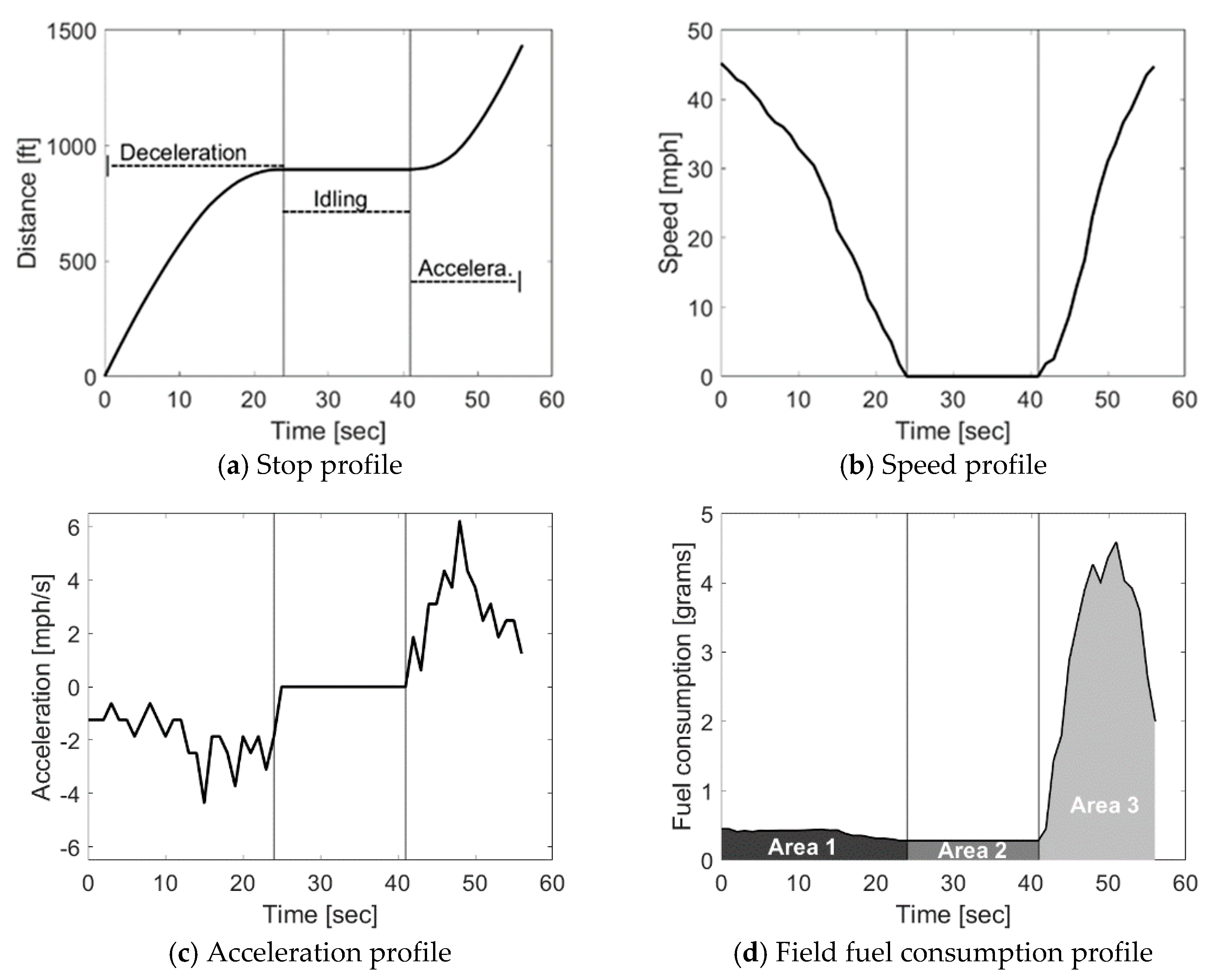
The stop penalty needed to reduce FC was derived based on the fuel consumed during the three driving modes of a complete stop at signalized intersections. These modes are deceleration, idling, and acceleration. An example of field vehicular trajectory of those modes is shown in Figure 1a. The change in speed during those modes can be represented by a Cruising Speed Stop Profile (CSSP), as displayed in Figure 1b. Cruising speeds before deceleration and after acceleration are not necessarily equal. In fact, field data processing, discussed later, showed that it is rare that a vehicle decelerates from a particular cruising speed and accelerates back to the exact original speed. The reality is that the cruising speed after accelerating can be lower or higher than the original cruising speed before stopping. Figure 1c depicts changes in acceleration during a stop event. Finally, the instantaneous FC changes over time during a CSSP are demonstrated in Figure 1d. The total FC of a CSSP is formulated in Equation (4) [23], where all units are identical and can be in gallons, liters, or grams:
where FCCSSP is total fuel consumed during a CSSP, FCD is fuel consumed during the deceleration mode, FCI is fuel consumed during the idling mode, and FCA is fuel consumed during the acceleration mode.
The K-factor is the number of seconds of delay that consume the same amount of fuel consumed by a stopping event. Hence, it is crucial to separately identify extra fuel consumed during a stopping event (deceleration and acceleration modes), represented as FCDA (FCD + FCA), from what is consumed during the stopped delay, represented as FCI. Thus, we can say that FCDA is equal to a constant (Ke) multiplied by the FCI, as expressed in Equation (5).
By rearranging Equation (5), the unitless constant (Ke) can be denoted as shown below:
The stopped delay varies based on the length of the red interval for a given phase. So, for this reason, the FCI is divided by the total idling time (TI) in seconds, as shown in Equation (7). This step is important to assign the number of seconds of stopped delay equivalent to a stopping event, which is the stop penalty (K-factor). The PI (Equation (1)) can then be called FC-PI (since it is derived to reduce FC) and is expressed as shown in Equation (8).
where Di is stopped delay on link i (seconds), Si is total stops on link i, and n is number of links in the network or links included in the optimization process.
2.2. Factors Impacting Stop Penalty
It is apparent from Equation (7) that the K-factor depends significantly on the operating conditions that impact the FC during the deceleration, idling, and acceleration modes of a stopping event. Such primary conditions include vehicle type, proportion of heavy vehicles in the fleet (because of their heavy masses [25]), driving behavior, road gradient, cruising speed, and aerodynamic effect. The individual and combined impacts of all the previously mentioned conditions on the stop penalty, based on simulation results, were documented elsewhere [24,26]. However, the impact of two additional factors (idling FC rate (FCI/TI) and deceleration duration (TD)) was not examined in the previous studies. On the one hand, higher FC rates (FCI/TI) result in lower K values, as it can be concluded from Equation (7). On the other hand, a longer deceleration duration causes a higher K value because the excess FC during the deceleration phase depends on the duration of the deceleration process, which depends on several factors, including the driver’s behavior and the traffic dynamics of the vehicle(s) in front of the stopping vehicle. Thus, regardless of how small the FC (per unit of time) during deceleration is, longer deceleration times mean more fuel consumed.
Therefore, the predictive models developed in this study are based on the combined impact of various vehicle types, cruising speeds, road gradients, driving behaviors (acceleration-deceleration rates), FC rate during idling, and deceleration durations. Besides their profound effect on the K-factor, these factors were chosen because they can be (mostly) acquired from the vehicular trajectories recorded via On-board diagnostics (OBD) readers in the field. It is worth mentioning that for cruising speed, road gradient, and driving behavior parameters, attention was given for the acceleration side of those parameters (e.g., speed after accelerating, grade while accelerating, and acceleration itself). That is because the same parameters during deceleration have an insignificant impact on the stop penalty, as discussed later in the paper.
2.3. Collection of Field Data
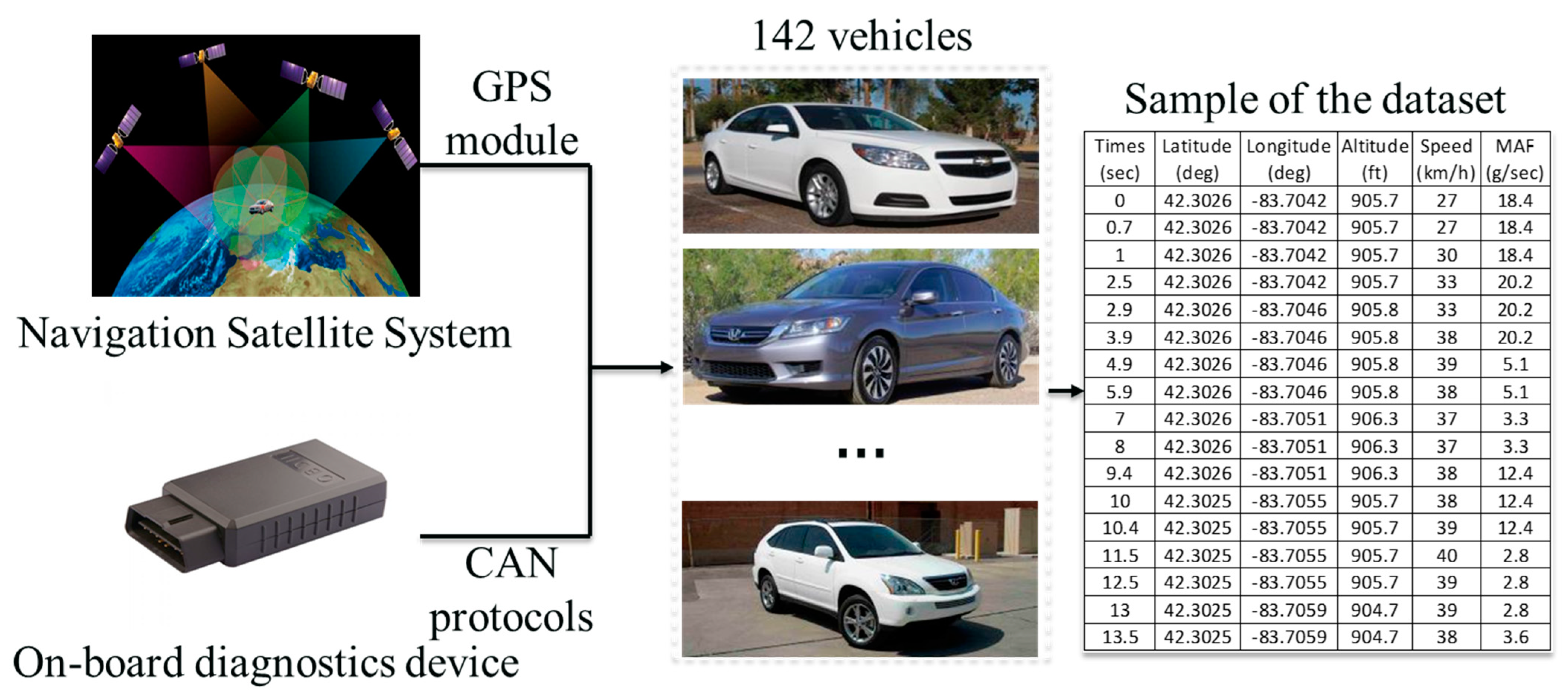
This study investigates the stop penalty by utilizing a dataset provided by the Department of Energy (DOE) [27] and collected by the Idaho National Lab [28]. The dataset includes vehicular trajectories of field trips lasting for 1850 h and covering 41,385 miles of various urban arterials in Michigan, which offers a wide range of collected FC rates under different operating conditions. InMetrics telemetry On-board diagnostics (OBD) recorder from ISAAC instruments (InMetrics telemetry, Ohio, United States) [29], combined with a Global Positioning System (GPS) module, was installed in the tested vehicles, and used to collect the field data. Although the OBD recorder can sample over 40 distinctive parameters with a frequency of up to 10 Hz, only eight parameters were included in the dataset. This study focused on the parameters latitude, longitude, altitude, speed, and mass airflow, and the last one was used to compute FC (more details below). The process of collecting the data with a sample of the utilized parameters are shown in Figure 2.
The authors decided to use this field dataset because it contains many CSSPs, it includes stops on uphill and downhill roadway sections, it has a fleet consisting of many vehicle types, and it encompasses various drivers with different driving behaviors. These characteristics made this dataset suitable to test the impact of various operating conditions on the K-factor. The following subsection discusses the preparation of field data that was followed to achieve the goal of the study.
2.4. Data Preparation
The DOE provided the dataset as a giant Comma-separated values (CSV) file; hence, it was necessary to divide the entire dataset into smaller subsets for easier handling. Each subset included trajectories for a single tested vehicle. Prior to commencing the data preparation, tested vehicles were classified into homogenous groups based on their properties that impact FC, especially based on vehicular engine sizes. The purpose of the classification was to combine the stop penalties computed for similar vehicles in one group as it is formidable to present the results for each vehicle. Following this step, a Python code was developed to extract all the CSSPs for each tested vehicle (discussed in Section 2.3) and determine the following parameters for each CSSP, cruising speeds, (i) right before decelerating and (ii) right after the end of accelerating; grades while decelerating and accelerating; idling FC rate; duration of deceleration stage; acceleration. In the end, the stop penalty was computed for all extracted CSSPs individually using Equation (7) and FC estimates recorded in the field.
2.4.1. Vehicle Classification
This section presents the vehicle clustering process. For the reader’s convenience, Table 1 summarizes the notation used in this subsection.
A total of 177 vehicle models with various Internal Combustion Engines (ICEs) were tested during the DOE field data collection campaign, including many vehicular styles (e.g., 2-Door, 4-Door, passenger van, minivan, and pickup). Examples of the vehicles included 1996 Toyota Corolla sedan, 2000 Ford Truck Windstar van, 2003 Lexus GS 300, 2006 Honda Civic, Audi A4 Quattro, 2014 Hyundai Tucson, and Mazda CX-3. The 2012 Ford Truck F250 Crew 4 × 4 was the heaviest and the most powerful vehicle with an 8-DSL 6.7 L T/C engine, while the 2014 Toyota Yaris with 4-FI 1.5 L engine was the lightest and one of the least powerful vehicles. Classifying the tested vehicles is a fundamental procedure that is required when dealing with FC and the K-factor concepts. This is because the amount of vehicular FC and the K-factor depend significantly on vehicle characteristics, such as vehicle make, year of manufacture, engine technology, engine size, and vehicle mass. This study categorizes vehicles on two levels, (i) based on its size and purpose, a vehicle is either an LDV or an LDT (this classification level is similar to how the state of art FC models such as the Comprehensive Modal Emission Model CMEM, Virginia Tech microscopic (VT-Micro) model, and Virginia Tech Comprehensive Power-based Fuel Consumption Model (VT-CPFM) VT-CPFM categorize their tested vehicles), and (ii) based on vehicular operating characteristics that impact FC, and such classification is done by using the k-prototype algorithm [30].
The k-means algorithm is efficient for classifying various datasets, thus widely utilized for many data mining applications [31,32]. The major drawback of the k-means is that it is primarily limited to numeric data because it minimizes the Euclidean distance measured between data points and means of clusters [30]. In contrast, the k-prototype algorithm is a data-mining technique that clusters objects with numeric and categorical attributes based on and with the same efficiency as the k-means paradigm [30]. The k-prototype method dynamically updates the k-prototypes to maximize the intra-cluster similarity of objects. The object similarity measure is derived from both numeric and categorical attributes. Thus, the k-prototype algorithm was utilized in this study to classify the 177 tested vehicles into seven categories that were similar in operating characteristics impacting FC. The classification process was based on a 177-by-n matrix that included several vehicle attributes, including the vehicle class, vehicle year, engine size and technology, and vehicle mass. The k-prototype algorithm aims at minimizing a total cost function (C) [30]:
The first term of the total cost function is the total cost on all numerical objects () in cluster i. is represented by the within-cluster sum of squares (WCSS), which is often defined as the Euclidean distance sum of squares between each object () and the mean point () of the centroid of cluster (i), as expressed in Equations (10) and (11).
The second term of Equation (9) () is represented as the number of mismatches between an object and each cluster prototype () of cluster (i), which can be represented as follows:
where is a set of all unique values in the categorical attribute j, and is the probability of categorical prototype () occurring in cluster i. Hence, in Equation (9) can be rewritten as:
where is a weight for categorical attributes for cluster l. Such weight is introduced to avoid favoring either type of attribute (numerical or categorical). The selection of a value was recommended in [30] as the average standard deviations of numeric attributes. It should be noted that categorical values are unitless, whereas the numerical values follow the unit of the attribute being clustered.
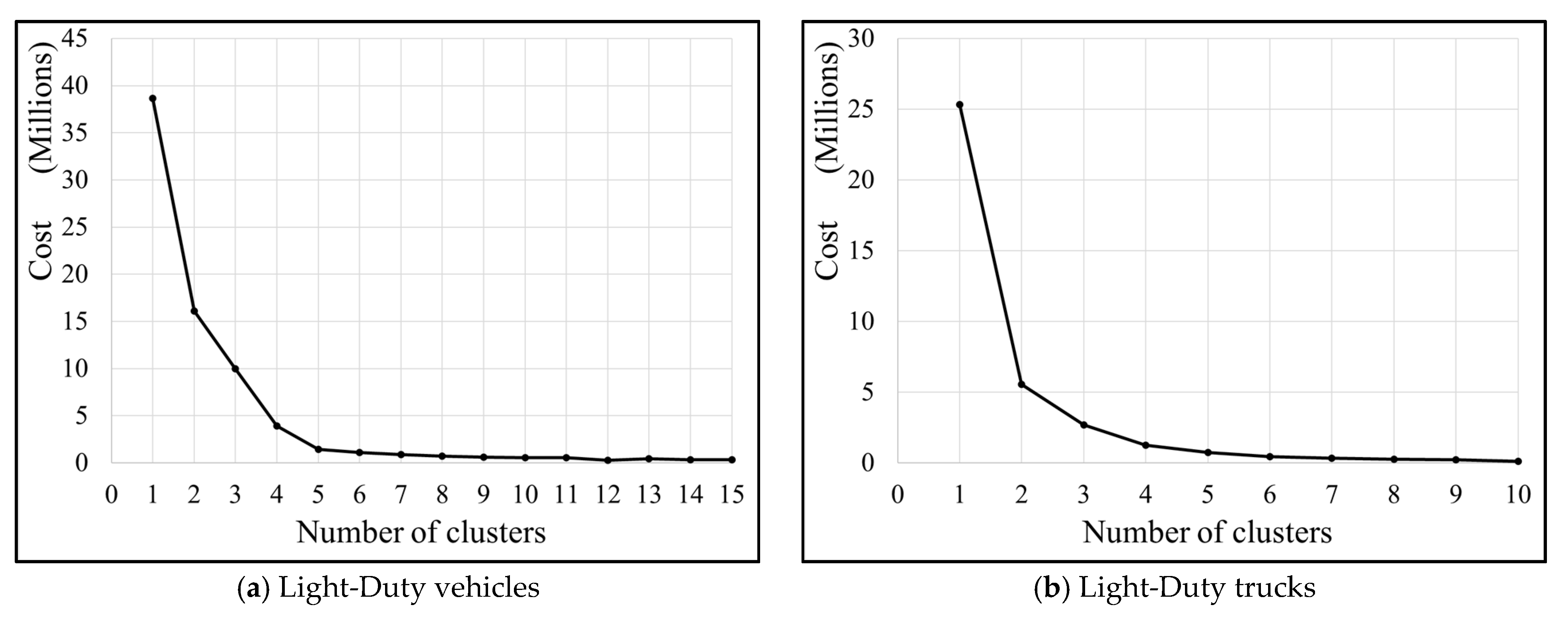
The k-prototype algorithm was applied to the data by using the Python programming language, allowing the user to input categorical and numerical vehicular characteristics for each tested vehicle to cluster vehicles into somewhat homogenous groups. When clustering the vehicles, all tested vehicles were initially divided into LDVs and LDTs because, as discussed earlier, LDVs and LDTs have significantly different FC characteristics. The number of LDV and LDT groups is determined by using the ‘Elbow method,’ which is based on the rate of ‘diminishing returns’. The Elbow method (Figure 3) uses the quality of clustering performance as a function of the number of groups to select a point at the elbow of the curve that indicates the optimum number of groups. From the result of the Elbow method in Figure 3, one can observe that four and three groups are suggested for LDVs and LDTs, respectively. Therefore, all tested vehicles were classified into seven groups identified as LDV1, LDV2, LDV3, LDV4, LDT1, LDT2, and LDT3.
2.4.2. Instantaneous Fuel Consumption Rates
Given that the OBD recorder provides the mass air flow (MAF) along with a timestamp, instantaneous FC rates can be derived from the recorded MAF [33,34]. Specifically, the instantaneous FC rates (gram/sec) were computed by using the MAF records, under the assumption that the stoichiometric (aka air-fuel) ratio is 14.7 [35]. The instantaneous FC can then be calculated using Equation (14). It should be noted that using a constant air-fuel ratio is not 100% accurate because the petroleum mixture will run lean or rich, depending on the power required by the engine [34,35]. Therefore, FC estimates from Equation (14) include a certain level of error. Although the air-fuel ratio can range from 6.1 to 20.1 for a gasoline engine [35], the vehicle’s catalytic converter and its management system work together to keep the stoichiometric ratio at 14.7. Therefore, assuming a stoichiometric ratio of 14.7 in this study is expected to have an insignificant impact on FC estimates, as shown in other studies [33,34], which are later used to compute the K-factor, as discussed in the following subsections.
where FC is the fuel consumption (grams/sec), a is the mass air flow (grams/sec), and s is the stoichiometric ratio equals to 14.7.
2.4.3. Cruising Speeds and CSSPs
The next step was to detect and extract CSSPs, for each tested vehicle, from the entire vehicular trajectories. Such a step started by detecting zero speeds (idling time) and then determining the two cruising speeds of a stop event. First, the cruising speed before starting the deceleration phase (referred to as initial speed hereafter), and second, the cruising speed after the accelerating phase (referred to as final speed hereafter). We define initial speed as the maximum speed at which a stopping vehicle starts to decelerate to zero speed. Similarly, the final speed is the maximum speed reached after accelerating before the vehicle reaches its initial speed or starts decelerating again. The initial and final speed definitions were used to develop a Python (Python Software Foundation, Haarlem, Netherlands) code to determine and extract each CSSPs from the vehicular trajectory data.
Initial data processing showed that some vehicles decelerating from an initial speed do accelerate for a short time (<2 s) before decelerating to zero. The opposite situation can happen during accelerating, where accelerating vehicles can decelerate for a short time due to queuing and then continue accelerating to their cruising speed. Therefore, the developed code accounted for such inconsistencies and determined the actual initial and final speeds to extract CSSPs.
After the initial and final speeds were determined for each CSSPs, the next step was to determine idling FC rate, decelerations and accelerations, deceleration’s duration, and road gradients. Idling FC rate is defined as an average FC in grams/sec during idling. Deceleration and acceleration are the rates of change in velocities from initial speed to zero and zero to the final speed, respectively. The following subsection explains the grade computation during the deceleration and acceleration phases.
2.4.4. Road Gradient
Road gradient during the deceleration mode was computed as an average value based on the difference in altitude between the point of initial speed and the point at which the vehicle reaches a zero speed. Similarly, the road gradient during the acceleration mode was computed based on the difference in altitude between the starting acceleration point (at zero speed) to the point at which the vehicle reaches its final speed.
Initial observation of the data showed that the altitude data are missing for several tested vehicles. Moreover, resolutions of some of the altitude data may not be sufficiently accurate for computational purposes. Thus, the missing altitude data of higher resolution were acquired, when needed, from the National Elevation Dataset available from the U.S. Geological Survey [36] (an agency in the US Department of the Interior) based on recorded latitude and longitude coordinates in the field.
Finally, the stop penalty was computed for all CSSPs from the field using Equation (15), which results from substituting Equations (7) and (14).
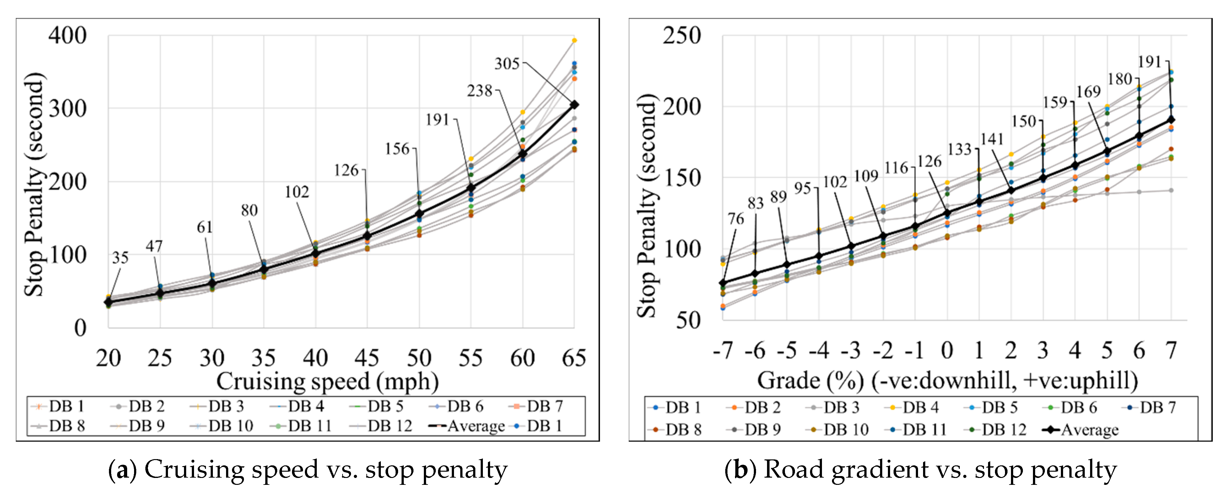
As mentioned previously, a recent simulation-based study [24] investigated the individual impact of multiple operating conditions (e.g., cruising speed and road gradient) on the K-factor (Figure 4). The study concluded that the K-factor varies significantly under various conditions. Thus, the K-factor should be a function of multiple factors. To achieve that, the following subsection explains the development of a series of predictive models to estimate the K-factor, considering the simultaneous impact of various factors.
2.5. Machine Learning (ML) Models
ML techniques have been used extensively in various transportation applications (e.g., [37]). This subsection presents an evolutionary computation (EC) technique to estimate the K-factor based on various operating conditions, such as vehicle type, cruising speed, road gradient, driving behavior, idling FC, and deceleration duration.
2.5.1. Multigene Genetic Programming
An EC method was used in this study because of two primary reasons, (i) EC models converge faster than a typical ML (e.g., neural network), and (ii) explicit mathematical formulations of the relationship between the K-factor and its independent factors can be derived [38,39,40,41]. The EC technique used in this study is called multigene genetic programming (MGGP). In MGGP, a single GP individual (program) is derived from a few genes, each of which is a tree expression [40,41]. Each model evolved by MGGP is a weighted linear combination of the outputs from a few GP trees. The trees are called “genes.” Figure 5 and Equation (16) show a typical 2-gene program evolved by MGGP. The inputs of the model are x2, x5, and x8. Several functions can be used for the evolution process (e.g., ×, −, +, Log, and √). The model is linear in the parameters for the coefficients , , and despite using nonlinear terms. As it is seen from Figure 5, the evolved model is a linear combination of nonlinear transformations of the predictor variables. Two important MGGP parameters that need significant attention are the maximum allowable number of genes and maximum tree depth. Restricting the tree depth mainly results in generating more compact models. The products of MGGP are profoundly nonlinear equations, reached after forming millions of preliminary models through a complex evolutionary process [42]. As described in previous sections, field data is used to generate the MGGP models, consisting of thousands of K values for a wide range of operating condition scenarios.
2.5.2. Development of MGGP Models
The initial inputs (or independent variables) included eight parameters for the training of the MGGP models, with the output (or dependent variable) being the stop penalty. Those independent variables are initial-final speeds, deceleration-acceleration grades, idling FC rates, deceleration-acceleration values, and the deceleration durations. Table 2 presents the input parameters with their minimum and maximum values. The vehicle type was also considered the ninth variable (to impact the stop penalty) by developing seven individual MGGP models for the seven vehicular groups described in the data preparation section. A few dozen of preparatory runs were conducted to determine the impactful input variables on the stop penalty. The outcomes revealed that decelerating grades and deceleration itself had an insignificant effect on the stop penalty. Accordingly, the MGGP models (seven models, one for each vehicular group) were developed by using only the six remaining variables, as given in Equation (17).
where is decelerating (initial) speed (mph), is accelerating (final) speed (mph), is accelerating grade (%), is idling FC rate (gram/sec), is decelerating duration (second), and is acceleration (ft/sec2).
CSSPs for each vehicle group were randomly partitioned into training, testing, and validation datasets based on the proportions 60%, 20%, and 20%, respectively. The best-performed models on the training and testing data were also assessed using a new (validation) dataset. GPTIPS toolbox [43], a free access MGGP training tool developed in MATLAB (MathWorks, Natick, MA, USA), was used to create the prediction models. Seven models were developed for the stop penalty, four for LDVs and three for LDTs. Table 3 shows the final attributes setting for the MGGP as recommended in previous studies [29,31,32].
Coefficient of determination (R2) and the root-mean-squared error (RMSE) were employed to judge the performance of the introduced models. RMSE and R2 equations are displayed in Equations (18) and (19).
where is computed K-factor for the output, is estimated K-factor for the output, is average computed K-factor, is average estimated K-factor, and is sample size.
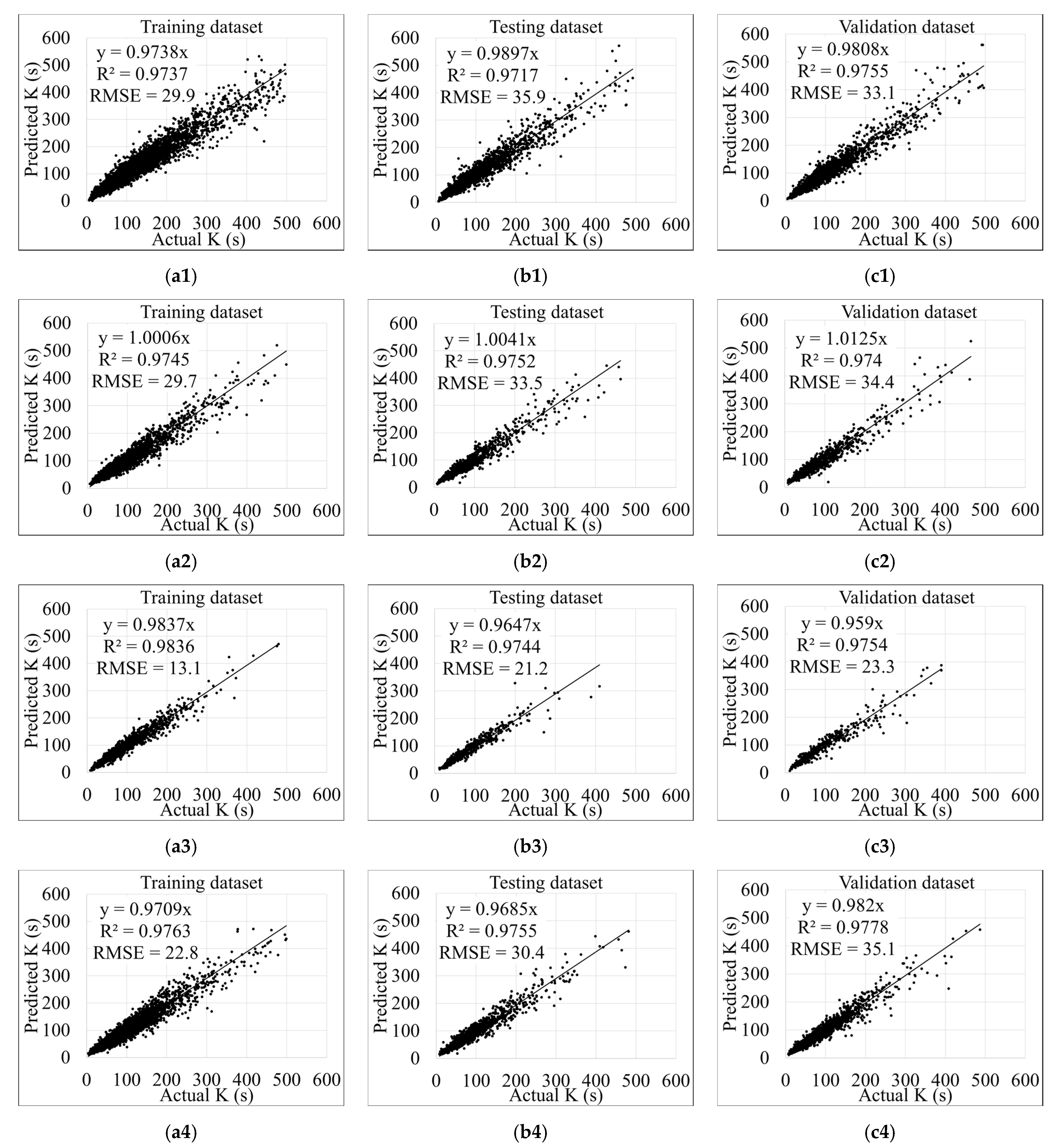
Equations (20)–(26) in Table 4 represent the stop penalty under various operating conditions for each vehicle group (LDV1, LDV2, LDV3, LDV4, LDT1, LDT2, and LDT3). These models were developed using (6188, 2604, 1379, 4073, 1588, 888, and 225) and (2063, 869, 460, 1358, 530, 269, and 75) sets of training and testing data, respectively.
3. Results and Discussion
3.1. Models Training, Testing, and Validation
Figure 6 and Figure 7 present the performance indices of the MGGP models on the training, testing, and validation datasets. As seen, the MGGP models have an excellent fitting and high coefficient of determination represented by R2 values of more than 0.96. It is important to note that the same training datasets (for the seven-vehicle groups) were used to develop multivariate linear regression models. The obtained R2 values were less than 0.35 for most of those regression models. Such poor performance of the conventional multivariate linear regression models can be explained by limitations of such statistical regression techniques. In most cases, the best linear or nonlinear models developed using the commonly used statistical approaches are obtained after controlling a few equations established in advance (30). Thus, such models cannot efficiently consider the interactions between the dependent and independent variables.
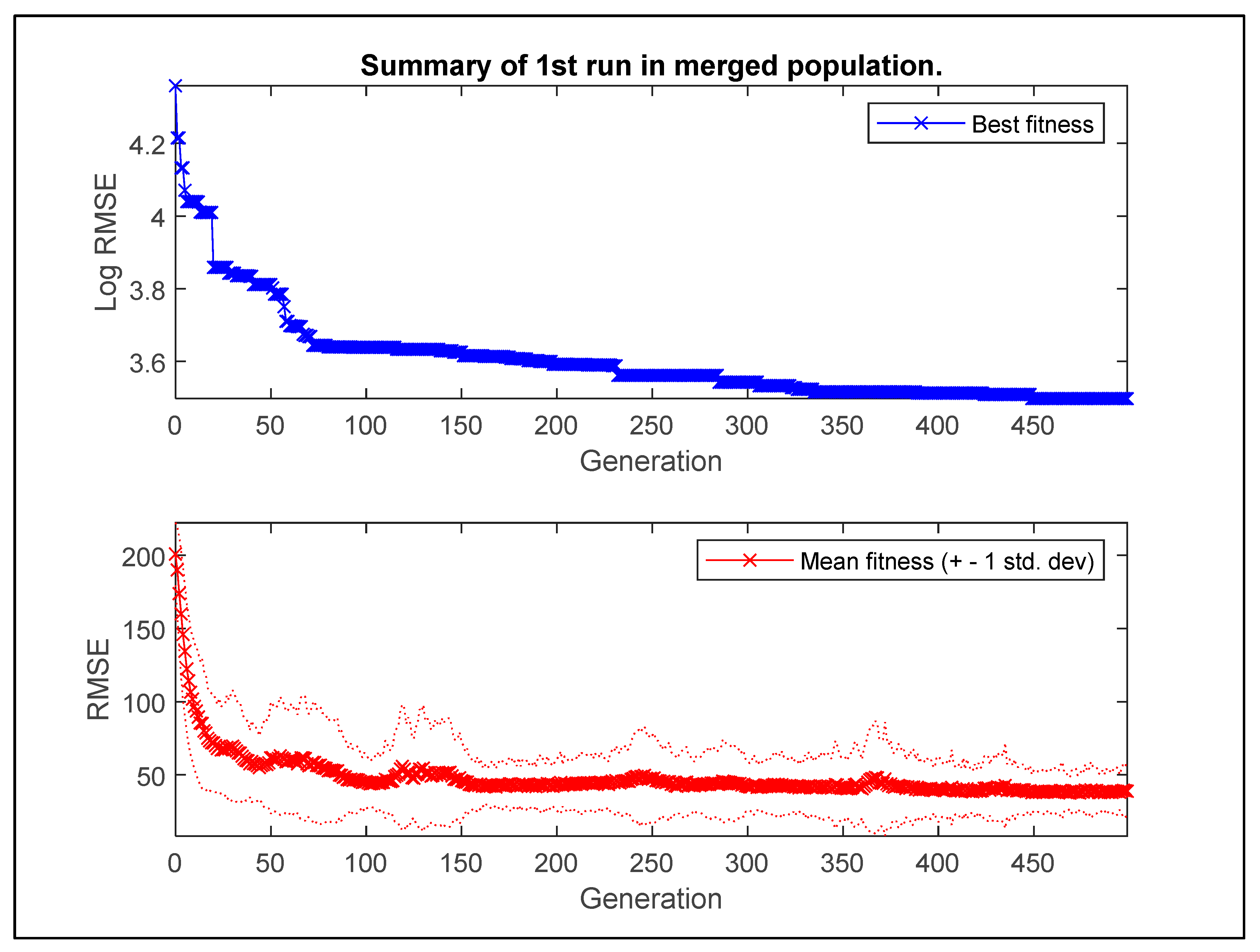
On the other hand, MGGP introduced completely new characteristics and traits and directly derived correlations without assuming prior forms of existing relationships. Figure 8 shows a simple summary example of a run in GPTIPS. The upper part and lower part of Figure 8 show the log10 value of the best RMSE and the mean RMSE achieved over the generations of a run. It is worth mentioning that the log10 value of the RMSE is the error metric that GPTIPS attempts to minimize over the training data.
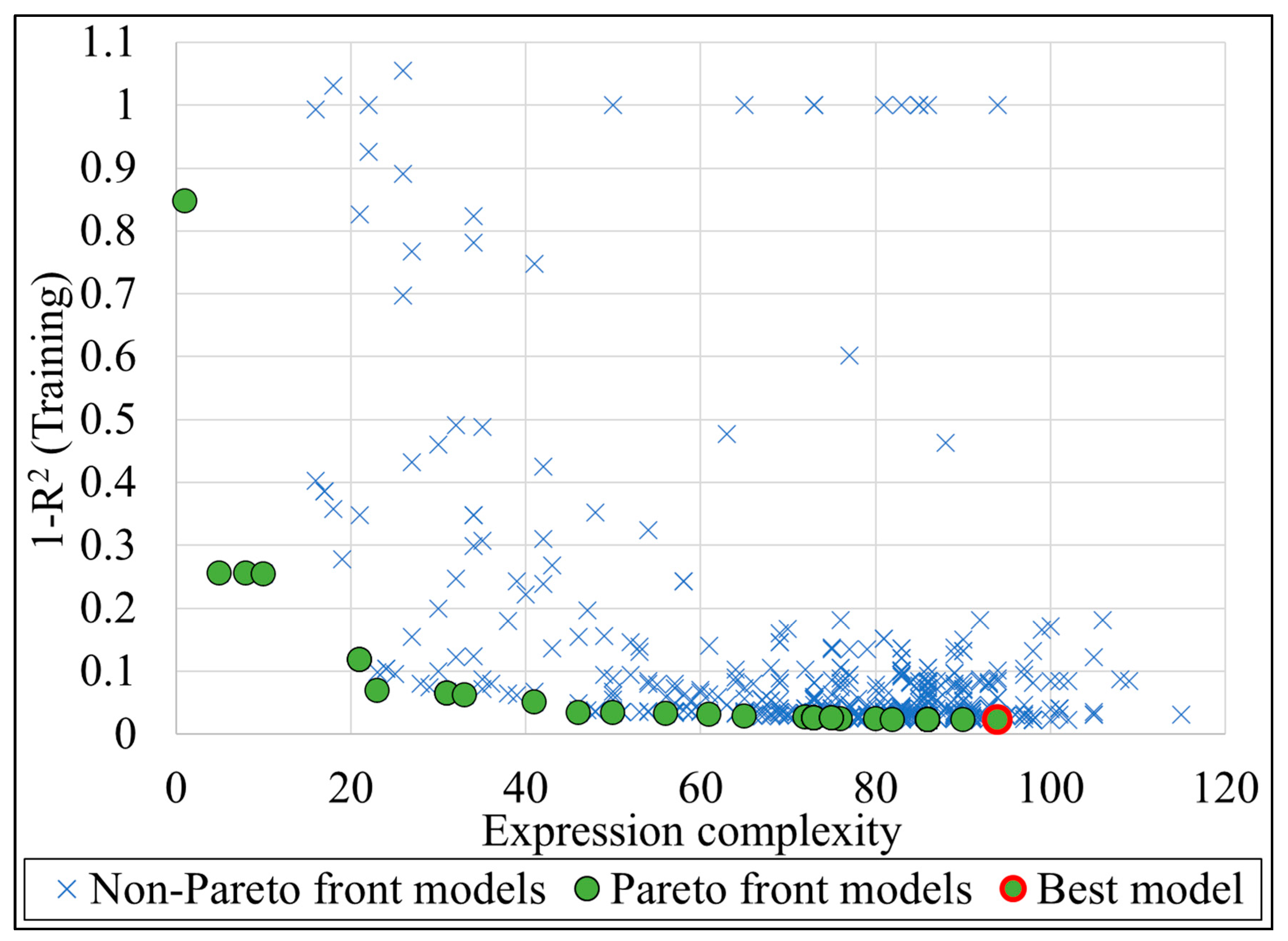
Figure 9 visualizes an example of the training procedure for minimizing the error and simplifying the complexity of the MGGP models during the evolutionary process. The green dots represent the Pareto front of models in terms of model performance and complexity. Blue Xs represent non-Pareto models. The red circled dot represents the best model in the population based on the R2 value on the training data. The final model for each vehicle group was selected based on two criteria, accuracy and model complexity. The developed models are validated with a fresh dataset to evaluate the generalization capability of the developed models. Figure 6(c1–c4) and Figure 7(c1–c3) show the acceptable performance of the models for the validation data.
3.2. Parametric Analysis
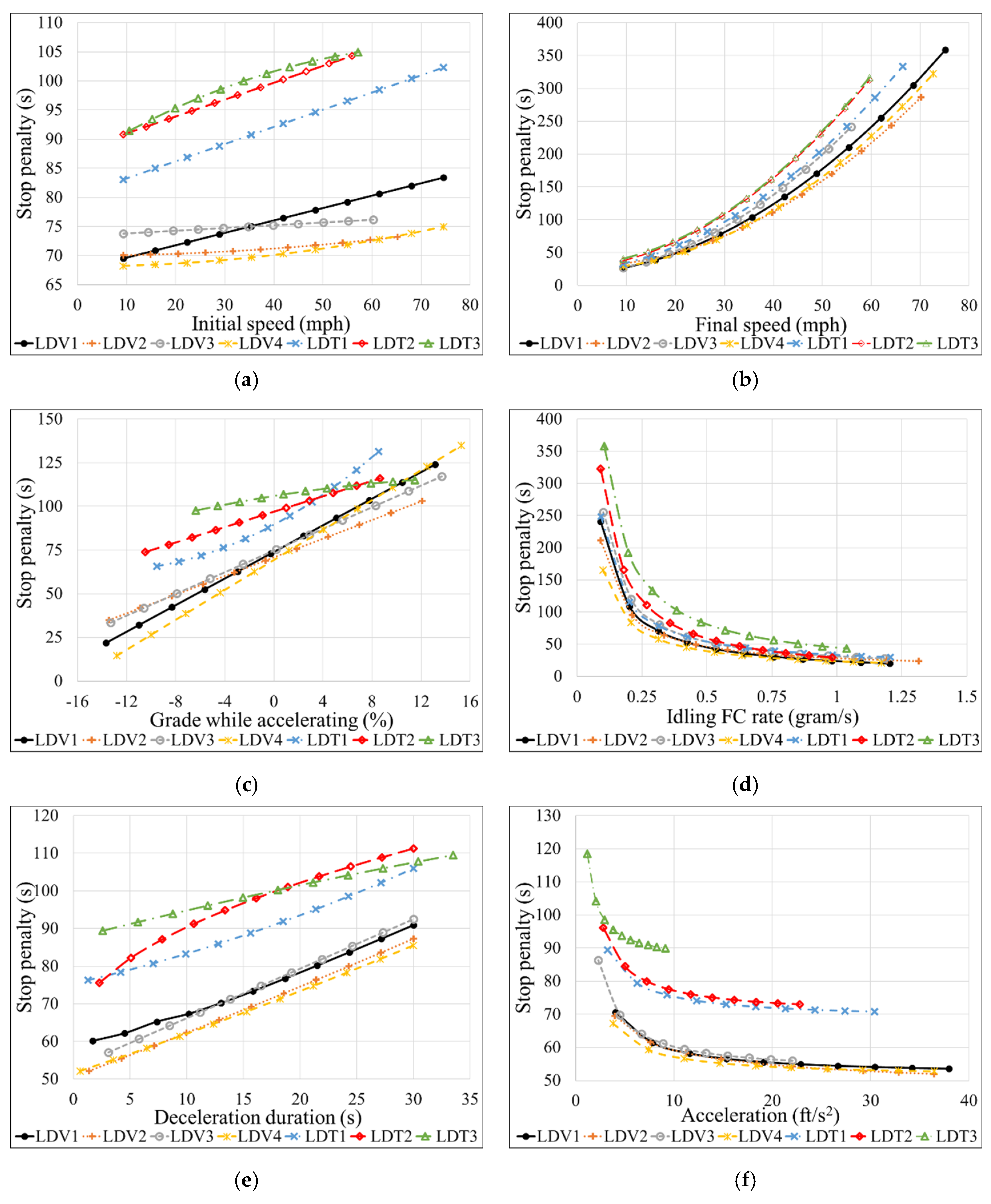
A parametric analysis was performed to investigate the impact of the tested independent factors on the stop penalty and to investigate the robustness of the developed models. This analysis was done by varying one parameter within a practical range, while other parameters were kept constant at their average values. Figure 10 shows the results of the parametric study for the best models. Figure 10 shows that all the studied factors had a significant impact on the value of the stop penalty. Some conditions (such as the final speed and idling FC rate) had a much more significant impact than the others (e.g., initial speed).
Figure 10 shows that the LDT groups had larger K values than those of the LDVs’. The difference in K value between LDT and LDV groups is most remarkable for the initial speed, accelerating grade, deceleration duration, and acceleration. The same difference is still observed for the other factors but with a smaller margin. Such findings can be mainly attributed to the vehicles’ masses, where heavier vehicles, represented by the LDTs, require more fuel (thus higher K value) than the lighter vehicles (LDVs) to operate under the same conditions of a stop event. On average and under various operating conditions, K values of LDTs were ~1.2–3 times higher than those of LDVs. It is expected that heavy-duty diesel vehicles (HDDVs) would have an even higher K value. It can also be observed from Figure 10 that the K value differs internally among the individual LDV and LDT groups. For instance, K values for LDV1 in Figure 10a range from 70–85 s, while LDV4′s range starts from 67–75 s. Thus, when computing the K value, it is crucial to pay considerable attention to the percentage of various vehicle types arriving at signalized intersections.
As shown in Figure 10a,b, the K-factor shows approximately linear and exponential relationships with the increase of the initial and final speeds, respectively. A comparison of the two relationships shows that the final speeds impact the K value much more than the initial speeds. As a result, various initial and final speeds lead to a K value between 67–105 and 15–350 s, respectively, for various vehicle types. The difference in the two ranges for the initial and final speeds is attributed to the fact that the amount of fuel consumed during acceleration is far larger than its counterpart during deceleration. Such a difference is important to be taken into account when computing the K-factor for left and right turns because, in those cases, initial and final speeds are often very different.
Regarding the grades, the findings show that grades during deceleration have a negligible impact on the K-factor, as mentioned in the previous sections. On the other hand, the road gradient on the acceleration side is found to correlate linearly with the K-factor. It is interesting to note that all seven models developed in this study cover a wide range of accelerating grades which can be as low as −13.5% and as high as 15% for most LDVs. In contrast, narrower ranges (−6% to 8%) were conducted for the LDTs, as shown in Table 2.
One of the most important findings of this study reveals an approximately quadrinomial relationship between idling FC rate and K-factor (Figure 10d). Such a relationship results in a K value of more than 250 s for some vehicle types at low idling FC rates. Most vehicles included in this study had an idling FC rate range between 0.1–1 g/s. There could be several reasons for such a wide range of idling FC rates, and engine size, mass, and ambient temperature are the most important ones. Since it is not easy to identify the idling FC rate for all vehicles stopping at signalized intersections, it is recommended that operating agencies use distributions of idling rates based on various vehicle types, various times of the day, and various climates zones.
Despite its minimal impact on the K-factor, it was necessary to show the relationship between FC during deceleration and the stop penalty. It is worth noting that the deceleration FC is highly unpredictable, as it depends on the driver’s characteristics (e.g., driving behavior and perception reaction time), geometrical characteristics of intersections, and the interactions (while breaking) with other vehicles. This study used deceleration durations to represent the deceleration FC. Figure 10e demonstrates that deceleration duration impacts the stop penalty linearly.
Surprisingly, higher accelerations were found to reduce the stop penalty, as illustrated in Figure 10f. This finding was unexpected and suggested that maybe the acceleration duration (required to reach the final speed) is more impactful than the aggressiveness of accelerating. This is speculated because higher accelerations require a shorter time to reach a particular speed. Therefore, caution and engineering judgment must be applied until further research is conducted because the findings of the impact of acceleration on the stop penalty might not be generalized or transferable to other datasets with the field vehicular trajectories.
3.3. Comparison of Stop Penalties from Various Studies
As mentioned in the introduction, only a few studies have computed the stop penalty, either by using FC collected in the field or FC estimates from simulated vehicular trajectories. This subsection discusses the stop penalty values from various studies [13,15,16,21,23,24] to address how the outcomes of this research may improve practices and policies when optimizing signal timings in urban corridors.
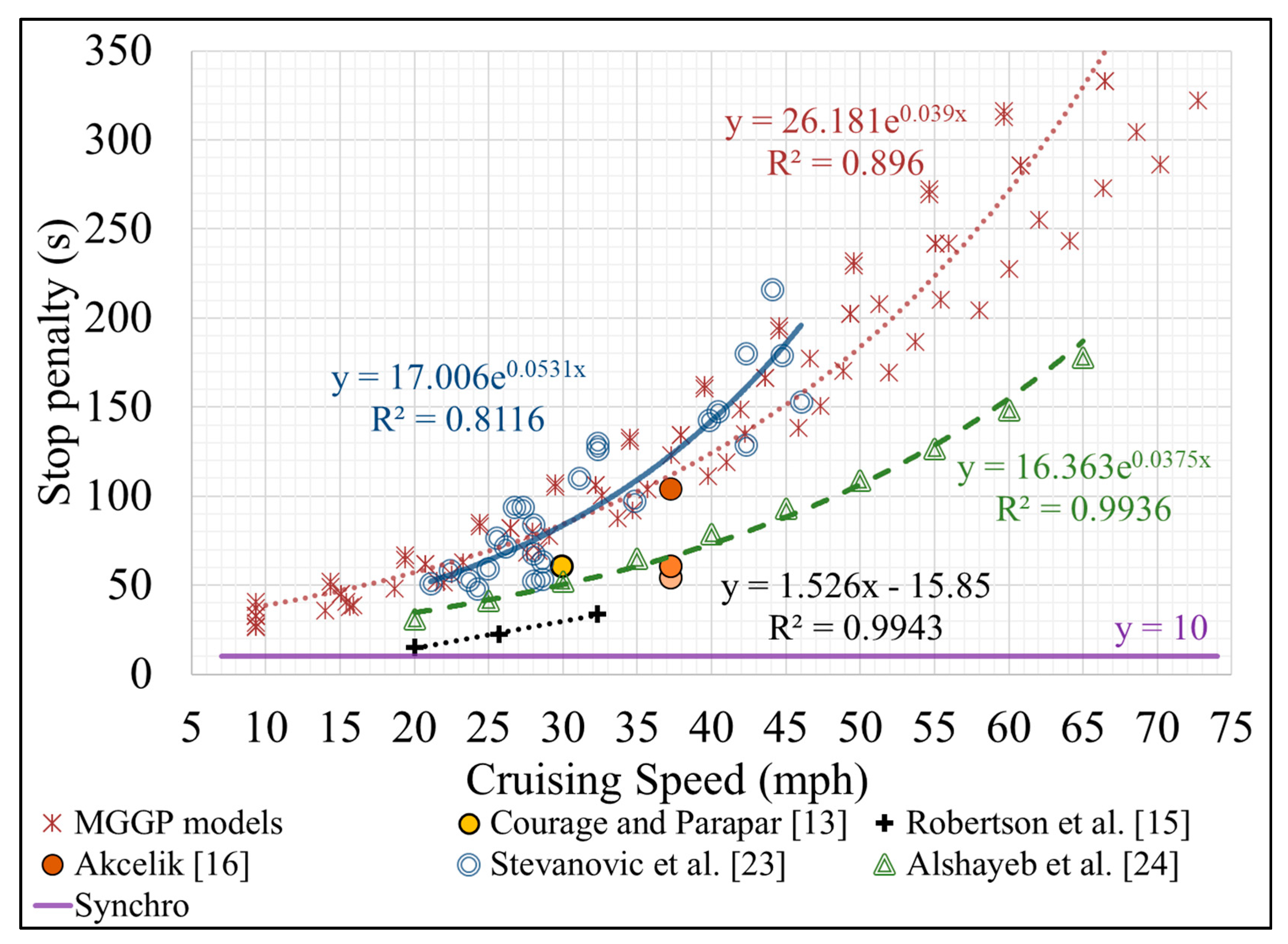
Considering that most of the evaluated studies report only the cruising speed (as a factor associated with the reported stop penalties), we developed in Figure 11 (with our best effort as data from various studies may not be 100% consistent) a set of relationships between the stop penalty and cruising speed from seven sources, MGGP models developed in this paper; “Synchro”—a widely used signal timing optimization tool [21]; field-based stop penalties reported by Courage and Parapar [13], Akcelik [16], Stevanovic et al. [23], and Robertson et al. [15]; simulation-based stop penalties from Alshayeb et al. [24].
Figure 11 shows that various studies show different trends, where most of them point to a positive impact of the speed on stop penalty. To be more precise, the studies can be classified, according to their trends, into two groups, (i) studies that report constant stop penalties (Courage and Parapar [13], Akcelik [16], and Synchro [21]) and (ii) studies that define the stop penalty as a function of—at least—the speed (field data covered in this research, Robertson et al. [15], Stevanovic et al. [23], and Alshayeb et al. [24]). The following paragraphs discuss in detail the results shown in Figure 11.
Courage and Parapar [13] were among the first to report a single stop penalty value (60 seconds) using FC measurements of a mixed fleet with a cruising speed of 30 mph and level grade, as reported by Claffey [44]. Akcelik [16] derived the stop penalties for three fleet distributions, one consisting exclusively of light vehicles, another of heavy vehicles, and one composite fleet with 10% of heavy vehicles, which resulted in K values of 54, 104, and 60 s, respectively. Those three stop penalty values are shown in Figure 11 as orange dots with various color intensities for a cruising speed of 37 mph. Reporting the speed at which the stop penalty was computed in both studies [13,16] indicates that the authors of those studies were aware of the importance of cruising speed on the stop penalty. However, the same studies did not collect field FC data for various vehicle types and other important factors (e.g., idling rate, grade), and for that reason, their reported stop penalties would not reflect the impact of those conditions.
Based on FC measurements from Robertson et al. [15], stop penalties show a positive linear trend with the cruising speed. However, that study also did not cover a wide range of cruising speeds (only three speeds) and was based on macroscopic FC measurements. Thus, the MGGP results seem to be more reliable because they were based on high-resolution FC measurements and covered a wide range of speeds.
Although a recent study by Stevanovic et al. [23] was conducted under some limitations (e.g., utilized a single vehicle, utilized a single driver, limited speed range of ~20–45 mph), the stop penalties from the MGGP models showed that the findings from Stevanovic et al. [23] are still quite valid. However, the MGGP models were still based on a much larger data set that includes many different vehicles and drivers and covers a much broader range of speeds (~10–75 mph).
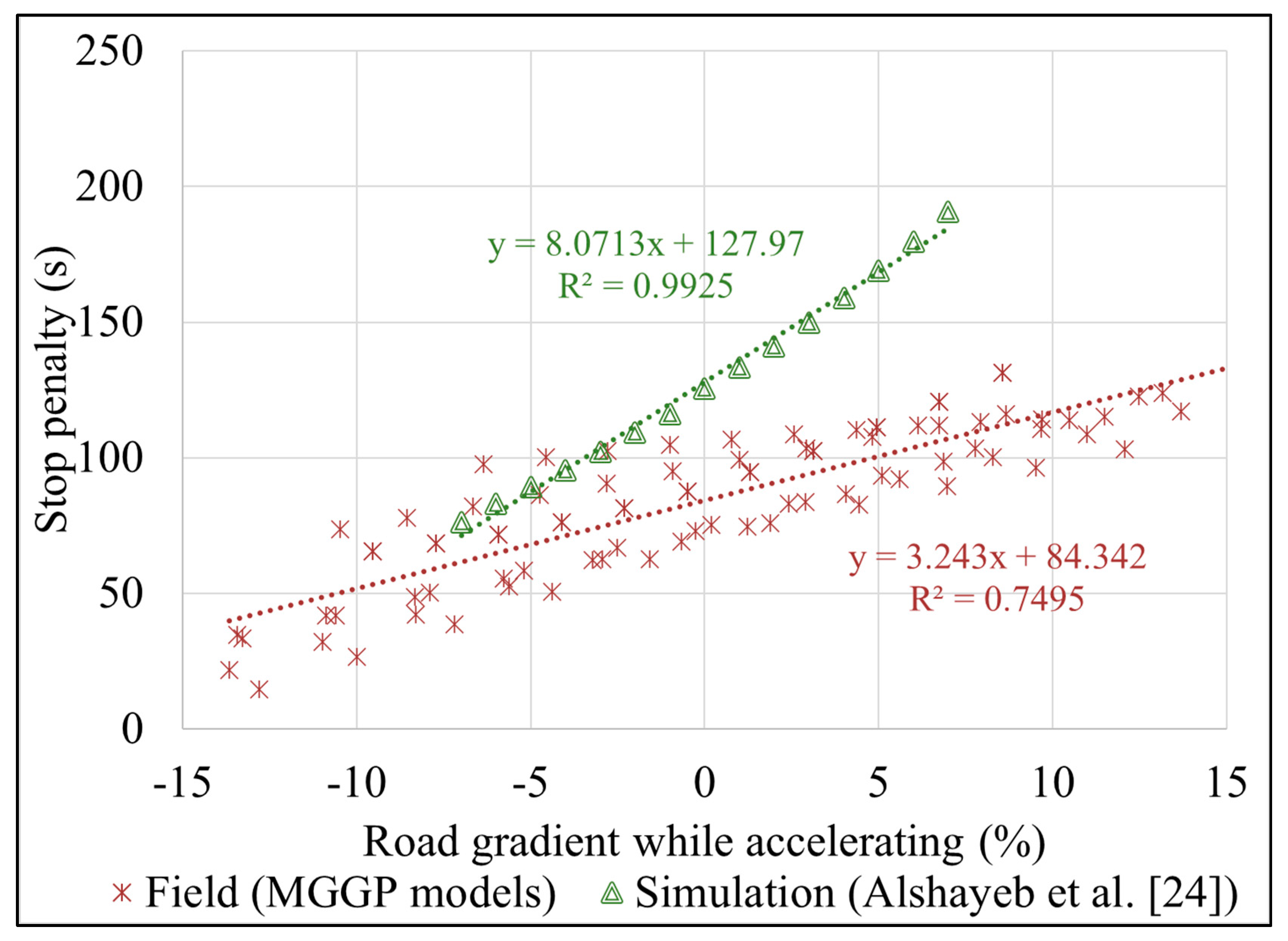
When comparing the MGGP stop penalties with those from the simulation models [24], Figure 11 shows that both data series depict the same trend (stop penalty correlates positively with the cruising speed), but it seems that the simulation-based stop penalties underestimate those from the field (e.g., either from this study or the results from Stevanovic et al. [23]). On the other hand, Figure 12, which compares the field and simulated stop penalties as functions of the road gradient, shows that the simulated data overestimated the field values. There could be several reasons for such differences between the field and simulated stop penalties (for both speeds and grades). One is the difference in the FC idling rate, which ranges from 0.1 to 1.3 g/sec in the field, whereas the range is smaller in the simulation (~0.20–0.6 g/sec). Or it could be that tested vehicle types in the field are very different from evaluated vehicle types in the simulation.
It is important to note that none of the previous studies, except for the one with simulated data [24], reported the impact of other factors (excluding cruising speed) on the stop penalty. The simulation-based study [24] covered the effect of multiple factors on the stop penalty, which are 15 vehicle types (make year 1990–2000), driving behavior represented by acceleration-deceleration functions, road gradient while accelerating (−7% to 7%, as shown in Figure 12), cruising speed (assuming equal speed before and after stopping), and aerodynamic effect from the wind. We also note that the simulation-based study [24] did not develop a prediction model to estimate the stop penalty considering various factors—it simply derived bivariate relationships between each individual factor (while other have been kept constant) and the stop penalty. In comparison to that study with simulated data, this work developed MGGP models that cover more than 170 modern vehicle types (1996–2017), driving behavior with higher resolution by separately including the deceleration and acceleration times, a larger range of road gradients (while accelerating) (~−14% to 14%), a broader range of cruising speeds, etc. Finally, the MGGP models are not bivariate—they represent multivariate correlations between the stop penalty (as dependent variable) and all of the listed impact factors.
Based on the previous discussion, the major unique features of the MGGP models can be summarized as follows:
- FC measurements were collected in the field, unlike Alshayeb et al. [24], whose stop penalties were simulation-based.
- Large number of LDVs and LDTs were included, whereas most previous studies used less than three vehicles.
- The tested fleet consisted of modern vehicles, whereas tested vehicles in the previous studies, except for Stevanovic et al. [23], are old for contemporary standards.
- Tested vehicles covered long distances, resulting in a significantly larger dataset than those used in the previous studies.
- The models cover multiple factors impacting the stop penalty (vehicle type, cruising speed, road gradient, FC idling rate, driving behavior, and decelerating duration), whereas most of the previous studies investigated only the impact of the cruising speed.
While transportation agencies in different regions in the US can utilize the developed models because they included a large fleet of commonly driven vehicles on US roads, it is unknown whether the K-factor might vary for various locations. However, it is expected that this will be the case, as the K-factor depends on the operating conditions of each specific area. For example, an area could have a large percentage of elderly or youthful population, whose driving behaviors are quite different. Thus, the K values for such a location can be significantly different from a demographically well-balanced area. Consequently, further research is needed to develop regional K values for multiple distinctive regions. That can be done by collecting floating vehicle data, including FC in the field, especially for critical signalized corridors in the region, or by modeling the operating conditions of those distinctive regions in traffic simulation and FC models and designing proper experiments to derive K values.
Another future research should utilize the emerging basic safety message (BSM) data from connected vehicles to calibrate the developed models. Further, in a fully vehicular connected traffic environment, the BSM data can be used to compute the current K value for each network movement and use such a value for real-time adjustment of traffic timing parameters. Finally, the BSM data can also be used to derive the K-factor based on user satisfaction instead of equivalent FC. In such a case, the K-factor is expected to be lower at movements where drivers may be more inclined to wait longer or be stopped more frequently (e.g., side streets) than at movements where drivers expect good progression (e.g., through movement on the major street).
4. Conclusions and Future Research
This study had two major objectives, (i) to assess the impact of the major operating conditions (vehicle type, cruising speed, road gradient, idling FC rate, deceleration duration, and driving behavior) on the stop penalty (K-factor) using vehicular trajectories and FC estimates collected from the field, and (ii) to develop valid EC models, namely MGGP, to formulate the stop penalty as a factor of various operating conditions.
An extensive real-world dataset from the field was used to develop predictive models for seven vehicular groups classified in this study. The performance of the developed models was evaluated by using testing and validation datasets. The models developed achieved high accuracy for the training, testing, and validation datasets.
A parametric study was also carried out to investigate the impact of the investigated factors on the stop penalty and to ensure the robustness of the developed models. The parametric study revealed that the stop penalty is positively correlated with all of the factors studied. Specifically, initial speed, grade while accelerating, and deceleration duration have linear relationships with the stop penalty, whereas the idling FC rates and accelerations have quadrinomial ones. Lastly, final speed seemed to impact the stop penalty exponentially. These findings suggest that, in general, the stop penalty is not a low constant value as widely thought in the traffic signal optimization community.
An implication of this study is the possibility of feasibly computing the K-factor by using the models developed in this study. It is recommended that traffic agencies should implement FC-based stop penalties in their signal timing optimization practices. Such implementation can be as simple as changing the value of K when optimizing signals using Synchro—or integrating the PI with correctly computed stop penalty as the objective function when optimizing signal timings utilizing various optimization techniques (e.g., genetic algorithm).
One limitation of the current study is that it does not analyze the impact of some other important factors affecting the stop penalty (e.g., pavement type and ambient temperature) due to their unavailability in the field dataset. However, this research has identified a few questions that require further investigation. Most importantly, a future study should investigate the actual applicability of various K-values (especially K > 250 s) for different movements of signalized intersections on the reduction of FC and other performance measures (e.g., progression and delay). In addition, one could develop a microscopic level ML model and evaluate and validate the performance of such a microscopic model. One could also integrate a vehicle dynamics model to consider vehicle throttle and braking levels to assure more accurate FC and emissions estimates. This would be particularly important when connected and automated vehicles are considered.
Author Contributions
Conceptualization, S.A., A.S. and B.B.P.; methodology, S.A., A.S. and B.B.P.; formal analysis, S.A., A.S. and B.B.P.; investigation, S.A., A.S. and B.B.P.; data curation, S.A., A.S. and B.B.P.; writing—original draft preparation, S.A., A.S. and B.B.P.; writing—review and editing, S.A., A.S. and B.B.P.; visualization, S.A., A.S. and B.B.P.; supervision, A.S. and B.B.P. All authors have read and agreed to the published version of the manuscript.
Funding
This research has been partially supported by funding from the Lake County (IL) Department of Transportation and the research contract on “Traffic Signal Optimization based on Fuel-consumption and Pollutant Emissions”.
Institutional Review Board Statement
Not applicable.
Informed Consent Statement
Not applicable.
Data Availability Statement
Data and codes used for this research could be shared with the research community on request to the corresponding author.
Acknowledgments
The authors want to thank the U.S. Department of Energy’s Vehicle Technologies Office and the Idaho National Laboratory for collecting and sharing the dataset used in this study. Also, we thank Tahnin Tariq from the Department of Civil and Environmental Engineering at the University of Pittsburgh for the help and discussions provided in developing the Python code mentioned in the data preparation section.
Conflicts of Interest
The authors declare no conflict of interest.
References
- McMichael, A.J.; Haines, J.A.; Slooff, R.; Sari Kovats, R.; World Health Organization. Climate Change and Human Health: An Assessment; World Health Organization: Geneva, Switzerland, 1996. [Google Scholar]
- Hannah, L. Climate Change Biology; Academic Press: Cambridge, MA, USA, 2021. [Google Scholar]
- Fast Facts on Transportation Greenhouse Gas Emissions [Internet]. EPA. Environmental Protection Agency; [updated on 8 July 2021; cited on 22 July 2021]. Available online: https://www.epa.gov/greenvehicles/fast-facts-transportation-greenhouse-gas-emissions (accessed on 3 November 2021).
- Pope, C.A., III; Burnett, R.T.; Thun, M.J.; Calle, E.E.; Krewski, D.; Ito, K.; Thurston, G.D. Lung cancer, cardiopulmonary mortality, and long-term exposure to fine particulate air pollution. JAMA 2002, 287, 1132–1141. [Google Scholar] [CrossRef] [Green Version]
- Rakha, H.; Ding, Y. Impact of stops on vehicle fuel consumption and emissions. J. Transp. Eng. 2003, 129, 23–32. [Google Scholar] [CrossRef]
- Alshayeb, S. Evaluation of Theoretical and Practical Signal Optimization Tools in Microsimulation Environment. Master’s Thesis, Florida Atlantic University, Boca Raton, FL, USA, 2019. [Google Scholar]
- Alshayeb, S.; Stevanovic, A.; Mitrovic, N.; Dimitrijevic, B. Impact of Accurate Detection of Freeway Traffic Conditions on the Dynamic Pricing: A Case Study of I-95 Express Lanes. Sensors 2021, 21, 5997. [Google Scholar] [CrossRef]
- Dobrota, N.; Stevanovic, A.; Mitrovic, N. Development of assessment tool and overview of adaptive traffic control deployments in the US. Transp. Res. Rec. 2020, 2674, 464–480. [Google Scholar] [CrossRef]
- Gavric, S.; Sarazhinsky, D.; Stevanovic, A.; Dobrota, N. Evaluation of Pedestrian Timing Treatments for Coordinated Signalized Intersections. In Proceedings of the Transportation Research Board 101st Annual Meeting, Washington, DC, USA, 9–13 January 2022. [Google Scholar]
- Stevanovic, A.; Dobrota, N.; Mitrovic, N. NCHRP 20-07/Task 414: Benefits of Adaptive Traffic Control Deployments-A Review of Evaluation Studies; Technical Report, Final Report; Transportation Research Board of the National Academies: Washington, DC, USA, 2019. [Google Scholar]
- Shayeb, S.A.; Dobrota, N.; Stevanovic, A.; Mitrovic, N. Assessment of Arterial Signal Timings Based on Various Operational Policies and Optimization Tools. Transp. Res. Rec. 2021. [Google Scholar] [CrossRef]
- Bauer, C.S. Some energy considerations in traffic signal timing. Traffic Eng. 1975, 45, 19–25. [Google Scholar]
- Courage, K.G.; Parapar, S.M. Delay and fuel consumption at traffic signals. Traffic Eng. 1975, 45, 23–27. [Google Scholar]
- Cohen, S.L.; Euler, G. Signal Cycle Length and Fuel Consumption and Emissions; Transportation Research Record: Thousand Oaks, CA, USA, 1978. [Google Scholar]
- Robertson, D.I.; Lucas, C.F.; Baker, R.T. Coordinating Traffic Signals to Reduce Fuel Consumption; Transport and Road Research Laboratory: London, UK, 1981. [Google Scholar]
- Akcelik, R. Fuel efficiency and other objectives in traffic system management. Traffic Eng. Control. 1981, 22, 54–65. [Google Scholar]
- “Brian” Park, B.; Yun, I.; Ahn, K. Stochastic optimization for sustainable traffic signal control. Int. J. Sustain. Transp. 2009, 3, 263–284. [Google Scholar] [CrossRef]
- Liao, T.Y. A fuel-based signal optimization model. Transp. Res. Part D Transp. Environ. 2013, 23, 1–8. [Google Scholar] [CrossRef]
- Stevanovic, A.; Stevanovic, J.; So, J.; Ostojic, M. Multi-criteria optimization of traffic signals: Mobility, safety, and environment. Transp. Res. Part C Emerg. Technol. 2015, 55, 46–68. [Google Scholar] [CrossRef] [Green Version]
- Road Research Laboratory. TRANSYT: A Traffic Network Study Tool. 1969. Available online: https://trid.trb.org/view/115048 (accessed on 3 November 2021).
- David, H.; John, A. Synchro Studio 7 User Guide; Trafficware, Ltd.: Houston, TX, USA, 2006; pp. 4–6. [Google Scholar]
- America, P.T. PTV Vistro User Manual; PTV AG: Karlsruhe, Germany, 2014. [Google Scholar]
- Stevanovic, A.; Shayeb, S.A.; Patra, S.S. Fuel Consumption Intersection Control Performance Index. Transp. Res. Rec. 2021. [Google Scholar] [CrossRef]
- Al Shayeb, S.; Stevanovic, A.; Effinger, J.R. Investigating Impacts of Various Operational Conditions on Fuel Consumption and Stop Penalty at Signalized Intersections. Int. J. Transp. Sci. Technol. 2021. [Google Scholar] [CrossRef]
- Ardalan, T.; Liu, D.; Kaisar, E. Truck Tonnage Estimation Using Weigh-In-Motion (WIM) Data in Florida. In Proceedings of the Transportation Research Board 99th Annual Meeting, Washington, DC, USA, 12–16 January 2020. [Google Scholar]
- Alshayeb, S.; Stevanovic, A.; Dobrota, N. Impact of Various Operating Conditions on Simulated Emissions-Based Stop Penalty at Signalized Intersections. Sustainability 2021, 13, 10037. [Google Scholar] [CrossRef]
- Department of Energy. Available online: https://www.energy.gov/ (accessed on 3 November 2021).
- Idaho National Laboratory. INL. 2021. Available online: https://inl.gov/ (accessed on 3 November 2021).
- Driver-Centric Fleet Management Solutions [Internet]. ISAAC Instruments. 2021 [updated 2021 Jul 9 cited 2021 Jul 22]. Available online: https://isaacinstruments.com/en/ (accessed on 3 November 2021).
- Huang, Z. Clustering large data sets with mixed numeric and categorical values. In Proceedings of the 1st Pacific-Asia Conference on Knowledge Discovery and Data Mining (PAKDD), Singapore, 23–24 February 1997; pp. 21–34. [Google Scholar]
- Yadav, J.; Sharma, M. A Review of K-mean Algorithm. Int. J. Eng. Trends Technol. 2013, 4, 2972–2976. [Google Scholar]
- Hartigan, J.A.; Wong, M.A. Algorithm AS 136: A k-means clustering algorithm. J. R. Stat. Soc. Ser. C (Appl. Stat.) 1979, 28, 100–108. [Google Scholar] [CrossRef]
- An, F.; Barth, M.; Norbeck, J.; Ross, M. Development of comprehensive modal emissions model: Operating under hot-stabilized conditions. Transp. Res. Rec. 1997, 1587, 52–62. [Google Scholar] [CrossRef] [Green Version]
- Park, S.; Rakha, H.; Ahn, K.; Moran, K. Virginia tech comprehensive power-based fuel consumption model (VT-CPFM): Model validation and calibration considerations. Int. J. Transp. Sci. Technol. 2013, 2, 317–336. [Google Scholar] [CrossRef] [Green Version]
- Hillier, V.A.; Coombes, P. Hillier’s Fundamentals of Motor Vehicle Technology; Nelson Thornes: Cheltenham, UK, 2004. [Google Scholar]
- National Geospatial PROGRAM. The National Map. (n.d.). Retrieved 12 September 2021. Available online: https://www.usgs.gov/core-science-systems/national-geospatial-program/national-map (accessed on 3 November 2021).
- Iqbal, M.S.; Ardalan, T.; Hadi, M.; Kaisar, E.I. Developing Guidelines for Implementing Transit Signal Priority (TSP) and Freight Signal Priority (FSP) Using Simulation Modeling and Decision Tree Algorithm. In Proceedings of the Transportation Research Board 100th Annual Meeting, Washington, DC, USA, 5–29 January 2021. [Google Scholar]
- Martínez-Ballesteros, M.; Troncoso, A.; Martínez-Álvarez, F.; Riquelme, J.C. Mining quantitative association rules based on evolutionary computation and its application to atmospheric pollution. Integr. Comput. Aided Eng. 2010, 17, 227–242. [Google Scholar] [CrossRef] [Green Version]
- Roy, R.; Bhatt, P.; Ghoshal, S.P. Evolutionary computation based three-area automatic generation control. Expert Syst. Appl. 2010, 37, 5913–5924. [Google Scholar] [CrossRef]
- Zhang, Q.; Barri, K.; Jiao, P.; Salehi, H.; Alavi, A.H. Genetic programming in civil engineering: Advent, applications and future trends. Artif. Intell. Rev. 2021, 54, 1863–1885. [Google Scholar] [CrossRef]
- Koza, J.R.; Koza, J.R. Genetic Programming: On the Programming of Computers by Means of Natural Selection; MIT Press: Cambridge, MA, USA, 1992. [Google Scholar]
- Gandomi, A.H.; Alavi, A.H. A new multi-gene genetic programming approach to nonlinear system modeling. Part I: Materials and structural engineering problems. Neural Comput. Appl. 2012, 21, 171–187. [Google Scholar] [CrossRef]
- Searson, D.P.; Leahy, D.E.; Willis, M.J. GPTIPS: An open source genetic programming toolbox for multigene symbolic regression. In Proceedings of the International Multiconference of Engineers and Computer Scientists, Hongkong, China, 17–19 March 2010; Volume 1, pp. 77–80. [Google Scholar]
- Claffey, P.J. Running Costs of Motor Vehicles as Affected by Road Design and Traffic; NCHRP Report; Transportation Research Board: Washington, DC, USA, 1971. [Google Scholar]
Figure 1.
Dynamics and kinematics of a stopped vehicle [24].
Figure 1.
Dynamics and kinematics of a stopped vehicle [24].

Figure 2.
Field data collection process.

Figure 3.
Determine optimal number of vehicle groups using the Elbow method.

Figure 4.
Impact of various speeds, grades, and driving behaviors (DB) on the K-factor [21].
Figure 4.
Impact of various speeds, grades, and driving behaviors (DB) on the K-factor [21].

Figure 5.
Typical 2-gene program evolved by MGGP with a maximum tree depth of 4.

Figure 6.
Predicted versus computed stop penalty of light-duty vehicle (LDV) groups: (1) LDV1, (2) LDV2, (3) LDV3, (4) LDV4, (a) training data, (b) testing data, (c) validation data.
Figure 6.
Predicted versus computed stop penalty of light-duty vehicle (LDV) groups: (1) LDV1, (2) LDV2, (3) LDV3, (4) LDV4, (a) training data, (b) testing data, (c) validation data.

Figure 7.
Predicted versus computed stop penalty of light-duty truck (LDT) groups: (1) LDT1, (2) LDT2, (3) LDT3, (a) training data, (b) testing data, (c) validation data.
Figure 7.
Predicted versus computed stop penalty of light-duty truck (LDT) groups: (1) LDT1, (2) LDT2, (3) LDT3, (a) training data, (b) testing data, (c) validation data.

Figure 8.
Example of a run summary shows reduction in RMSE with the number of generations.

Figure 9.
Example of the fluctuations in the training error while searching for the best model.

Figure 10.
Parametric analysis of the developed models. (a) Initial speed vs. stop penalty; (b) Final speed vs. stop penalty; (c) Accelerating grade vs. stop penalty; (d) Idling FC rate vs. stop penalty; (e) Deceleration duration vs. stop penalty; (f) Acceleration vs. stop penalty.
Figure 10.
Parametric analysis of the developed models. (a) Initial speed vs. stop penalty; (b) Final speed vs. stop penalty; (c) Accelerating grade vs. stop penalty; (d) Idling FC rate vs. stop penalty; (e) Deceleration duration vs. stop penalty; (f) Acceleration vs. stop penalty.


Figure 12.
Stop penalty vs. road gradient from the field and simulation [24].
Figure 12.
Stop penalty vs. road gradient from the field and simulation [24].


Table 1.
Nomenclature.
| Variable | Description |
|---|---|
| Total cost function of the k-prototype algorithm | |
| Number of clusters | |
| Cluster | |
| Cost of assigning numerical objects in cluster i | |
| Cost of assigning categorical objects in cluster i | |
| Within-cluster sum of squares | |
| Numerical object number j in cluster i | |
| Mean point of the centroid of cluster (i) | |
| Number of numerical objects in each cluster i | |
| Categorical prototype number j in cluster i | |
| Number of categorical objects in cluster i | |
| Set of all unique values in the categorical attribute j | |
| LDV | Light-duty vehicle |
| LDT | Light-duty truck |
Table 2.
Values of the input parameters used in the training sets.
| Input Parameter | LDV1 Model | LDV2 Model | LDV3 Model | LDV4 Model | LDT1 Model | LDT2 Model | LDT3 Model | |||||||
|---|---|---|---|---|---|---|---|---|---|---|---|---|---|---|
| Min | Max | Min | Max | Min | Max | Min | Max | Min | Max | Min | Max | Min | Max | |
| (mph) | 9.32 | 74.56 | 9.32 | 65.24 | 9.32 | 60.27 | 9.32 | 74.56 | 9.32 | 74.56 | 9.32 | 55.92 | 10.56 | 57.17 |
| (mph) | 9.32 | 75.19 | 9.32 | 70.21 | 9.32 | 55.92 | 9.32 | 72.7 | 9.32 | 66.49 | 9.32 | 59.65 | 9.32 | 59.65 |
| (%) | −13.67 | 13.16 | −13.43 | 12.08 | −13.29 | 13.69 | −12.8 | 15.28 | −9.54 | 8.55 | −10.48 | 8.65 | −6.36 | 11.49 |
| (gram/sec) | 0.09 | 1.2 | 0.09 | 1.314 | 0.1 | 1.18 | 0.1 | 1.17 | 0.09 | 1.21 | 0.09 | 0.98 | 0.1 | 1.04 |
| (sec) | 1.7 | 30 | 1.4 | 30 | 3.1 | 30 | 0.6 | 30 | 1.3 | 30 | 2.3 | 30 | 2.6 | 33.5 |
| (ft/sec2) | 0.28 | 37.97 | 0.39 | 36.45 | 0.1 | 22.02 | 0.16 | 36.45 | 0.24 | 30.38 | 0.59 | 22.78 | 0.3 | 9.11 |
Table 3.
Optimal MGGP attributes setting.
| Attribute * | Options/Value |
|---|---|
| Function set | +, −, x, /, log, sqrt, square |
| Population size | 800 |
| Number of generations | 500 |
| Maximum number of genes allowed in an individual | 6 |
| Maximum tree depth | 4 |
| Tournament size | 80 |
| Tournament type | Pareto (probability = 1) |
| Elite fraction | 0.7 |
| Number of inputs | 8 |
| Constants range | [−10, 10] |
| Complexity measure | Node count |
* All attributes are labeled as they are defined in the GPTIPS toolbox manual [43].
Table 4.
Mathematical formulations of the MGGP models.
| Model | Equation # |
|---|---|
| LDV1 | |
| (20) | |
| LDV2 | |
| (21) | |
| LDV3 | |
| (22) | |
| LDV4 | |
| (23) | |
| LDT1 | |
| (24) | |
| LDT2 | |
| (25) | |
| LDT3 | |
| (26) |
Publisher’s Note: MDPI stays neutral with regard to jurisdictional claims in published maps and institutional affiliations. |
© 2021 by the authors. Licensee MDPI, Basel, Switzerland. This article is an open access article distributed under the terms and conditions of the Creative Commons Attribution (CC BY) license (https://creativecommons.org/licenses/by/4.0/).
Share and Cite
MDPI and ACS Style
Alshayeb, S.; Stevanovic, A.; Park, B.B. Field-Based Prediction Models for Stop Penalty in Traffic Signal Timing Optimization. Energies 2021, 14, 7431. https://doi.org/10.3390/en14217431
AMA Style
Alshayeb S, Stevanovic A, Park BB. Field-Based Prediction Models for Stop Penalty in Traffic Signal Timing Optimization. Energies. 2021; 14(21):7431. https://doi.org/10.3390/en14217431
Chicago/Turabian StyleAlshayeb, Suhaib, Aleksandar Stevanovic, and B. Brian Park. 2021. "Field-Based Prediction Models for Stop Penalty in Traffic Signal Timing Optimization" Energies 14, no. 21: 7431. https://doi.org/10.3390/en14217431
Note that from the first issue of 2016, this journal uses article numbers instead of page numbers. See further details here.