Determination of Semi-Empirical Models for Mean Wave Overtopping Using an Evolutionary Polynomial Paradigm


Abstract
:1. Introduction
2. Average Wave Overtopping Assessment in Existing Literature
2.1. Goda (2009)
2.2. Mase et al. (2013)
2.3. EurOtop (2018)
2.3.1. Breaking and Non-breaking Wave Conditions
2.3.2. Very (shallow) Foreshores
2.4. Gallach (2018)
- aGallach = 0.0109 − 0.035(1.05 − cot α) and aGallach = 0.109 for cot α > 1.5;
- bGallach = 2 + 0.56(1.5 − cot cot α)1.3 and bGallach = 2 for cot α > 1.5; and
- cGallach = 1.1
3. Scaling Laws in Wave Overtopping
3.1. Volume Flux and Deficit in Freeboard
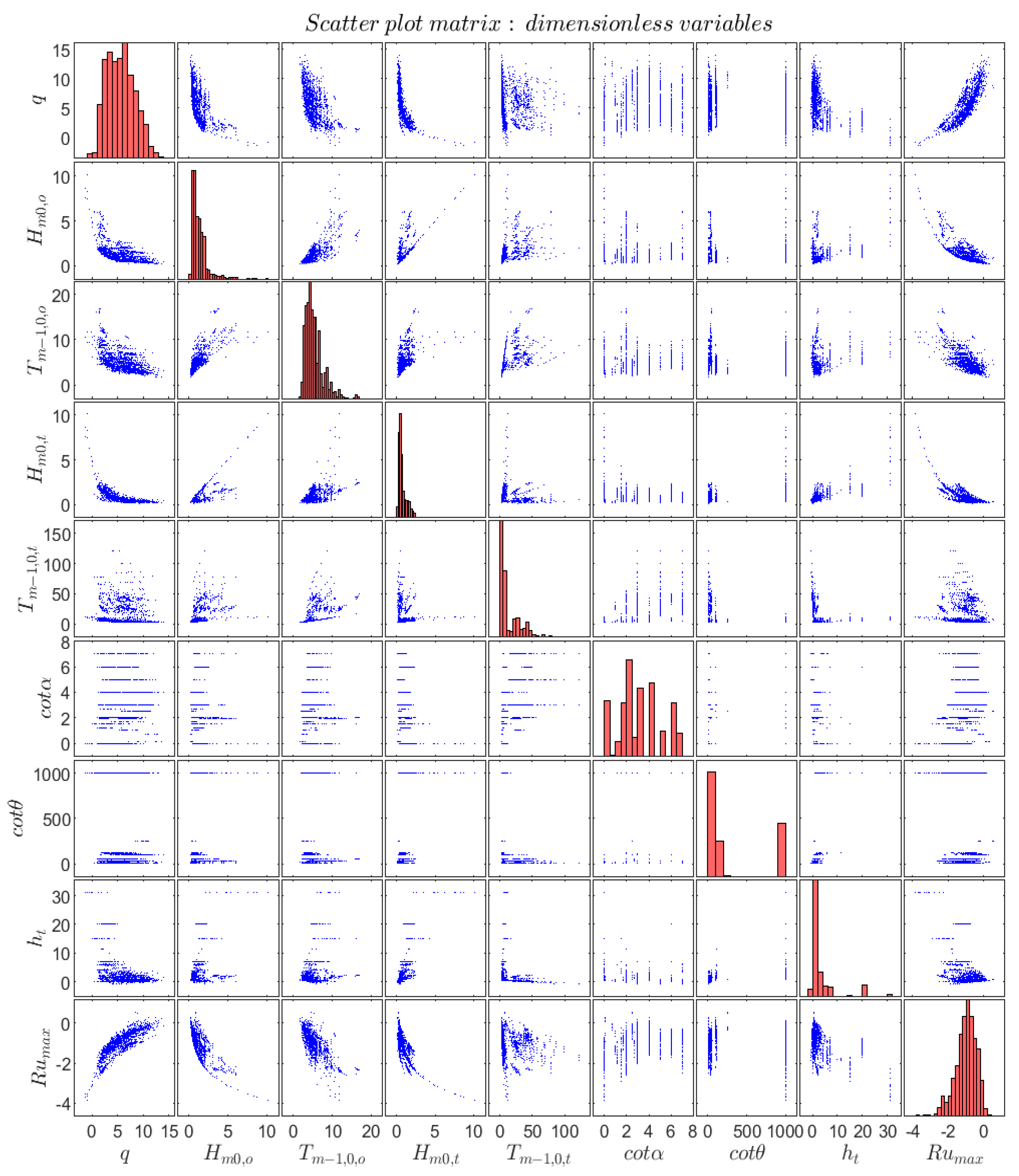
3.2. Dimensional Analysis
- (1)
- Q* = 4π2q/gHm0,oTm−1,0,o, based on [26], see Equation (14): deep-water wave characteristics are employed, after having verified that there is almost no difference (R2 = 99%) between the volume flux calculated employing the deep-water wave height and period with the one calculated based on local wave conditions at the toe.
- (2)
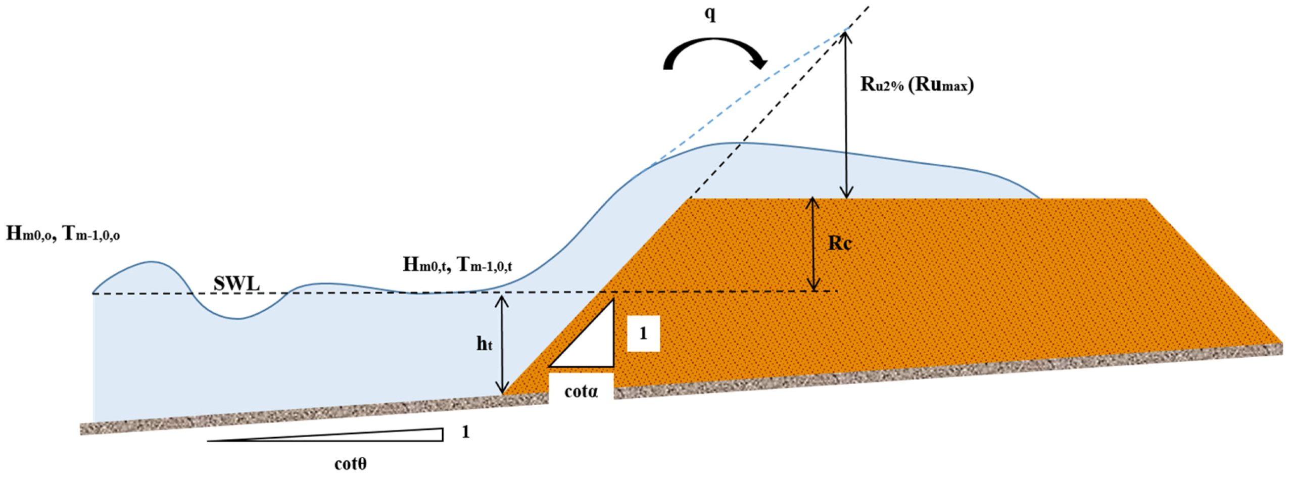
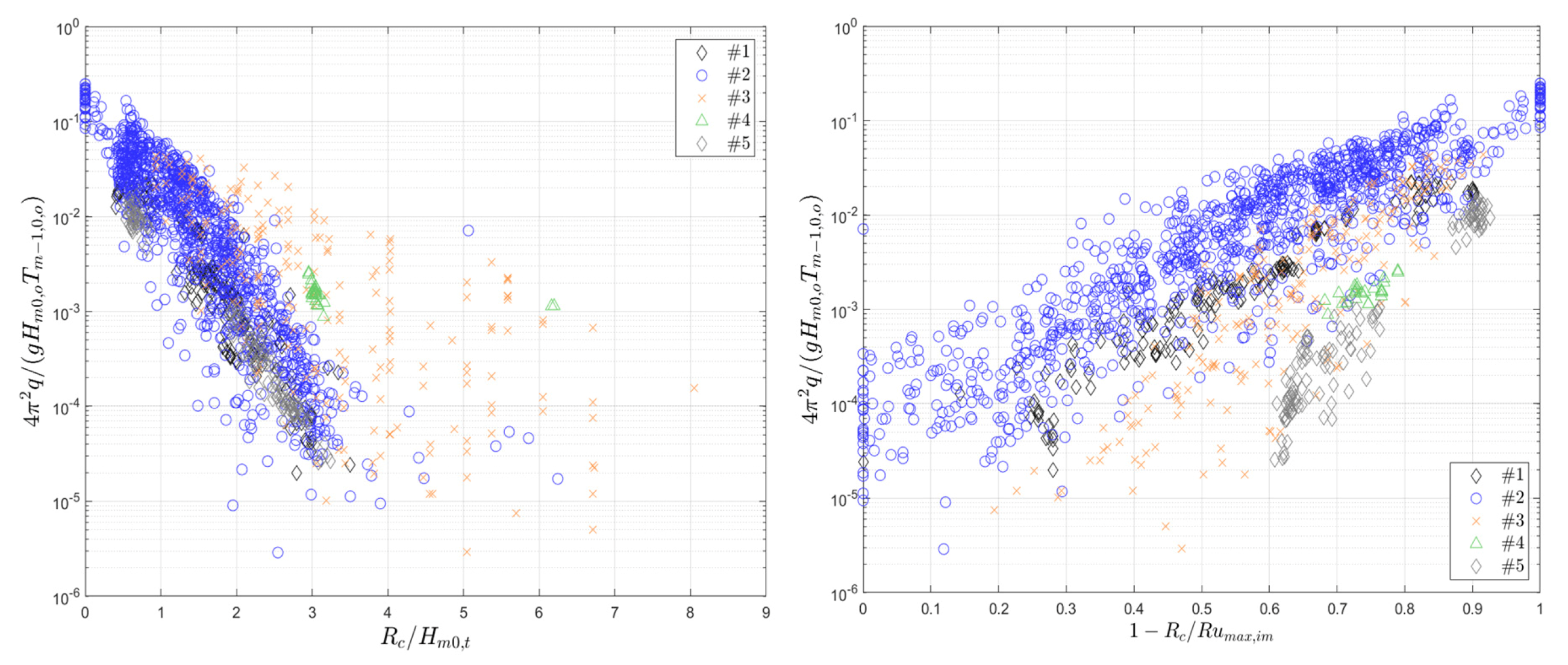
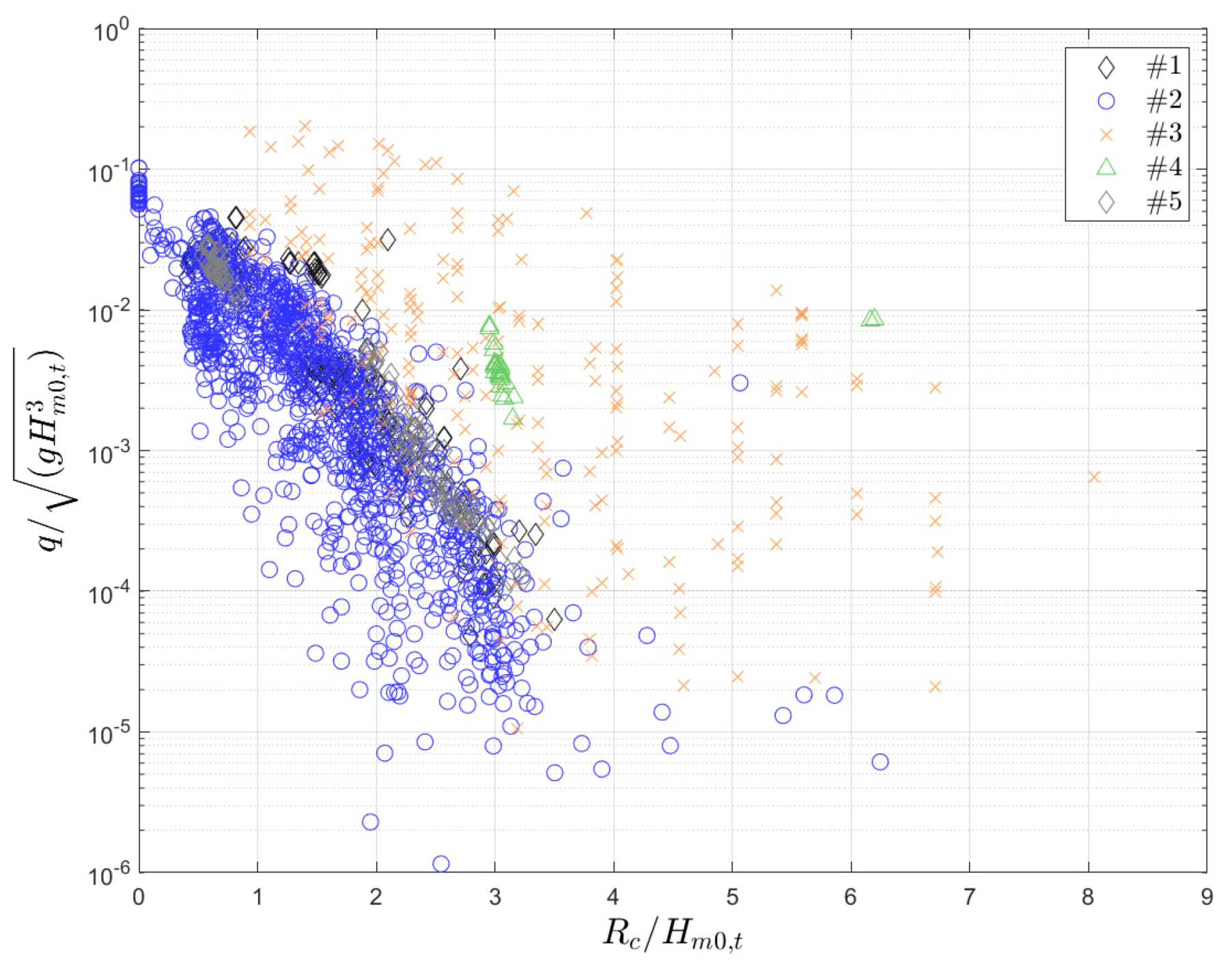
- Dimensionless freeboard, Rc/Hm0,t.
- (3)
- In [22] and [26], the overtopping is proved to be a function of the deficit of the freeboard, namely 1-Rc/Rumax, rather than the dimensionless freeboard. Notice that we use here the maximum run-up according to [22]. Considering the maximum run-up, the effects of wave periods, foreshore, and dike slope on overtopping discharge are included, as also in [13].
- (4)
- The slope parameter proposed in [27], β = θTm−1,0,o√(g/Hm0,o), is employed to consider the influence of long waves generated by the presence of mild slopes on wave overtopping.
- (5)
- (6)
- The ratio between the local water depth, the dike toe, and the local wave height, ht/Hm0,t, is considered as it was proven to have an influence on overtopping discharge [1], see Equations (2)–(3).
- (7)
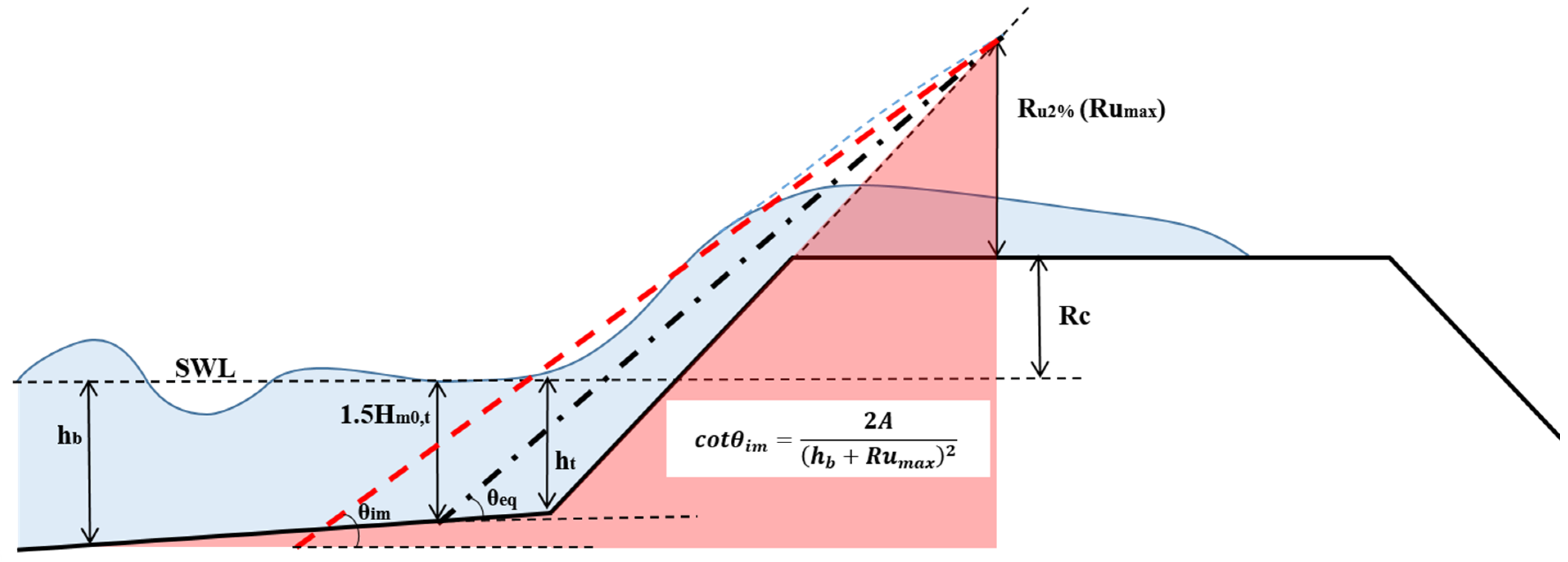
- The combined effect of the foreshore slope and dike slope is taken into account by considering the equivalent slope defined in [13] and expressed as cotθeq. As an alternative, the imaginary slope described in [22] and expressed as cotθim will be considered. By means of Evolutionary Polynomial Regression (EPR) application, the influence of the two conceptual slopes on the assessment of mean overtopping discharge will be evaluated and discussed.
- (8)
4. Methodology
4.1. The Evolutionary Polynomial Regression Paradigm
4.2. Model Performance
5. Experimental Datasets for Fitting Overtopping Formula
- EurOtop [19] database: the new extended database comprises about 13,500 tests on wave overtopping and extends the original CLASH database [40]. The tests include different dike geometries and kinds of structures, 14% of which represent smooth dikes. By excluding cases with zero overtopping, oblique waves, berms, or storm walls and considering only core data, finally 1128 data have been extracted.
- Data described in [13] and corresponding to tests on sea dikes with shallow foreshores. The tests correspond to five different experimental campaigns carried out at Flanders Hydraulics Research, in Antwerp, and at the Department of Civil Engineering of Ghent University, in Ghent (both in Belgium). These experimental campaigns were conducted to study the influence of mild foreshore slopes and very or extremely shallow water conditions on wave overtopping and loading on smooth sea dikes. The geometry of the dikes resembled typical layouts from the Belgian coast.
- Data from [41] corresponding to coastal defenses in Japan built in extremely shallow foreshores or on land (emergent toe), namely seawalls with slopes of 1:3, 1:5, and 1:7 with uniform foreshore slope of either 1:10 or 1:30. A Bretschneider–Mitsuyasu spectrum was used to generate random wave trains, differently from other datasets here employed, where a JONSWAP spectrum was employed.
- Data from [42] corresponding to the experimental campaign carried out in the multi-directional wave basin, at Flanders Hydraulics Research. A 1:2 sloping dike after a 1:35 foreshore slope was employed. All data correspond to cases with mild foreshore slope (β < 0.62) in very and extremely shallow water conditions (ht/Hm0,o < 1). The experimental campaign was conceived to characterize the overtopping discharge of long- and short-crested waves proceeding very obliquely with respect to the dike crest. For the present study, only perpendicular long-crested wave cases are considered.
- Data from Altomare et al. (under review) [43], where steep foreshore (β > 0.62) is used in combination with a rather steep dike (1:1) and very or extremely shallow waters (ht/Hm0,o < 1). The datasets include cases with crests larger than 0, which have been excluded from the present analysis. The experiments were carried out at the Maritime Engineering Laboratory of Universitat Politècnica de Catalunya – BarcelonaTech (LIM/UPC), in Barcelona, Spain. The scope of the experimental campaign was to measure the overtopping flow properties and analyze the related safety of pedestrian standing on the promenade of a sea dike.
6. A Set of Unified Formulas for the Preliminary Assessment of Wave Overtopping on Smooth Sea Dikes and Vertical Walls
EPR Setting and Results
7. Discussion
8. Conclusions
- Mean overtopping discharge is scaled by the volume flux, including both wave height and period ([26]): dimensionless discharge can be defined as Q* = 4π2q/gHm0,oTm−1,0,o. In this way, the wave period is always considered as an explanatory variable for wave overtopping assessment also for those cases where it is usually not taken into account; see Equation (9) for non-breaking waves.
- Employing deep-water wave characteristics rather than local wave characteristics at the dike toe to define the volume flux and, consequently, the scaling law for overtopping, leads to differences that are negligible. The reader can employ either the former ones or the latter ones, depending on the availability and accuracy of the employed information.
- EPR analysis confirms that an exponential structure, the most employed in literature (see [19]), leads to the best model representation.
- Both the dimensionless freeboard, Rc/Hm0,t, and the deficit in freeboard, 1-Rc/Rumax, are key explanatory variables for wave overtopping assessment. The main difference is that the definition of the deficit in freeboard requires the assessment of wave run-up, which is not only depending on the wave height but also on the wave period, local water depth, foreshore slope, and dike slope.
- Therefore, the study confirms previous findings from [13,22,23], and partly from [12], where other variables such as dike and foreshore slope and local water depth play an important role for the calculation of mean discharge rates. By combination these variables in one equivalent or imaginary slope concept, the model accuracy increases.
- EPR results confirm that the imaginary or equivalent slopes provided improve the estimate of mean discharge values, confirming somehow the physical meaning of such concepts. Overtopping reduces when the slope (defined as a cotangent of the angle with the horizontal) increases (heavier wave braking and dissipation over the foreshore slope).
Author Contributions
Funding
Conflicts of Interest
Disclaimer
References
- Sandoval, C.; Bruce, T. Wave Overtopping Hazard to Pedestrians: Video Evidence from Real Accidents in Coasts, Marine Structures and Breakwaters 2017; ICE Virtual Library: London, UK, 2018; pp. 501–512. [Google Scholar] [CrossRef]
- Mares-Nasarre, P.; Argente, G.; Gómez-Martín, M.E.; Medina, J.R. Overtopping layer thickness and overtopping flow velocity on mound breakwaters. Coast. Eng. 2019, 154. [Google Scholar] [CrossRef]
- Nørgaard, J.Q.H.; Lykke Andersen, T.; Burcharth, H.F. Distribution of individual wave overtopping volumes in shallow water wave conditions. Coast. Eng. 2014, 83, 15–23. [Google Scholar] [CrossRef]
- Victor, L.; van der Meer, J.W.; Troch, P. Probability distribution of individual wave overtopping volumes for smooth impermeable steep slopes with low crest freeboards. Coast. Eng. 2012, 64, 87–101. [Google Scholar] [CrossRef]
- Zanuttigh, B.; van der Meer, J.; Bruce, T.; Hughes, S. Statistical Characterisation of Extreme Overtopping Wave Volumes. In From Sea to Shore—Meeting the Challenges of the Sea; ICE Publishing: London, UK, 2014; pp. 442–451. [Google Scholar]
- van Bergeijk, V.M.; Warmink, J.J.; van Gent, M.R.A.; Hulscher, S.J.M.H. An analytical model of wave overtopping flow velocities on dike crests and landward slopes. Coast. Eng. 2019, 149, 28–38. [Google Scholar] [CrossRef] [Green Version]
- Schüttrumpf, H.; Oumeraci, H. Layer thicknesses and velocities of wave overtopping flow at seadikes. Coast. Eng. 2005, 52, 473–495. [Google Scholar] [CrossRef]
- Quvang, J.; Nørgaard, H.; Lykke, T.; Burcharth, H.F.; Jan, G. Analysis of overtopping flow on sea dikes in oblique and short-crested waves. Coast. Eng. 2013, 76, 43–54. [Google Scholar] [CrossRef]
- Romano, A.; Bellotti, G.; Briganti, R.; Franco, L. Uncertainties in the physical modelling of the wave overtopping over a rubble mound breakwater: The role of the seeding number and of the test duration. Coast. Eng. 2015, 103, 15–21. [Google Scholar] [CrossRef]
- Williams, H.E.; Briganti, R.; Pullen, T. The role of offshore boundary conditions in the uncertainty of numerical prediction of wave overtopping using non-linear shallow water equations. Coast. Eng. 2014, 89, 30–44. [Google Scholar] [CrossRef]
- Owen, M.W. Design of Seawalls Allowing for Wave Overtopping; Report No. EX 924; Hydraulics Research: Wallingford, UK, 1980. [Google Scholar]
- Gallach Sanchez, D. Experimental Study of Wave Overtopping Performance of Steep Low-Crested Structures; Ghent University: Ghent, Belgium, 2018. [Google Scholar]
- Altomare, C.; Suzuki, T.; Chen, X.; Verwaest, T.; Kortenhaus, A. Wave overtopping of sea dikes with very shallow foreshores. Coast. Eng. 2016, 116, 236–257. [Google Scholar] [CrossRef]
- Van der Meer, J.W.; Bruce, T. New Physical Insights and Design Formulae on Wave Overtopping at Sloping and Vertical Structures. J. Waterw. Port Coast. Ocean Eng. 2013, 140. [Google Scholar] [CrossRef] [Green Version]
- Van Doorslaer, K.; De Rouck, J.; Audenaert, S.; Duquet, V. Crest modifications to reduce wave overtopping of non-breaking waves over a smooth dike slope. Coast. Eng. 2015, 101, 69–88. [Google Scholar] [CrossRef]
- Chen, W.; van Gent, M.R.A.; Warmink, J.J.; Hulscher, S.J.M.H. The influence of a berm and roughness on the wave overtopping at dikes. Coast. Eng. 2020, 156, 103613. [Google Scholar] [CrossRef]
- Troch, P.; Geeraerts, J.; Van de Walle, B.; De Rouck, J.; Van Damme, L.; Allsop, W.; Franco, L. Full-scale wave-overtopping measurements on the Zeebrugge rubble mound breakwater. Coast. Eng. 2004, 51, 609–628. [Google Scholar] [CrossRef]
- Van Gent, M.R.A. Physical Model Investigations on Coastal Structures with Shallow Foreshores: 2d Model Tests with Single and Double-Peaked Wave Energy Spectra; Deltares (WL): Delft, The Netherlands, 1999. [Google Scholar]
- Van der Meer, J.W.; Allsop, N.W.H.; Bruce, T.; De Rouck, J.; Kortenhaus, A.; Pullen, T.; Schüttrumpf, H.; Troch, P.; Zanuttigh, B. Manual on Wave Overtopping of Sea Defences and Related Structures. An. Overtopping Manual Largely Based on European Research, but for Worldwide Application; EurOtop, 2018; Available online: www.overtopping-manual.com (accessed on 24 July 2020).
- Allsop, W.; Bruce, T.; Pearson, J.; Besley, P. Wave overtopping at vertical and steep seawalls. Proc. Inst. Civ. Eng. Marit. Eng. 2005, 158, 103–114. [Google Scholar] [CrossRef] [Green Version]
- Victor, L.; Troch, P. Wave Overtopping at Smooth Impermeable Steep Slopes with Low Crest Freeboards. J. Waterw. Port Coast. Ocean Eng. 2012, 138, 372–385. [Google Scholar] [CrossRef]
- Mase, H.; Tamada, T.; Yasuda, T.; Hedges, T.S.; Reis, M.T. Wave Runup and Overtopping at Seawalls Built on Land and in Very Shallow Water. J. Waterw. Port Coast. Ocean Eng. 2013, 139, 346–357. [Google Scholar] [CrossRef]
- Goda, Y. Derivation of unified wave overtopping formulas for seawalls with smooth, impermeable surfaces based on selected CLASH datasets. Coast. Eng. 2009, 56, 385–399. [Google Scholar] [CrossRef]
- Tamada, T.; Inoue, H.; Inoue, M. Proposal of diagrams for the estimation of wave overtopping rate on gentle slope-type seawall and consideration on time-related variation. Proc. Civ. Eng. Ocean 2001, 17, 311–316. [Google Scholar] [CrossRef]
- Goda, Y. A performance test of nearshore wave height prediction with CLASH datasets. Coast. Eng. 2009, 56, 220–229. [Google Scholar] [CrossRef]
- Ibrahim, M.S.I.; Baldock, T.E. Swash overtopping on plane beaches – Reconciling empirical and theoretical scaling laws using the volume flux. Coast. Eng. 2020, 157, 103668. [Google Scholar] [CrossRef] [Green Version]
- Hofland, B.; Chen, X.; Altomare, C.; Oosterlo, P. Prediction formula for the spectral wave period Tm−1,0 on mildly sloping shallow foreshores. Coast. Eng. 2017, 123. [Google Scholar] [CrossRef] [Green Version]
- Haykin, S. Neural Networks: A Comprehensive Foundation; Prentice Hall: Upper Saddle River, NJ, USA, 1999. [Google Scholar]
- Koza, J.R. Genetic programming as a means for programming computers by natural selection. Stat. Comput. 1994, 4, 87–112. [Google Scholar] [CrossRef]
- Davidson, J.W.; Savic, D.; Walters, G.A. Method for the identification of explicit polynomial formulae for the friction in turbulent pipe flow. J. Hydroinform. 1999, 1, 115–126. [Google Scholar] [CrossRef]
- Davidson, J.W.; Savic, D.; Walters, G.A. Approximators for the Colebrook-White Formula Obtained through a Hybrid Regression Method; Taylor & Francis, Inc.: Abingdon, UK, 2000; pp. 983–989. [Google Scholar]
- Draper, N.R.; Smith, H. Applied Regression Analysis; John Wiley & Sons: New York, NY, USA, 1966; 407 S., 43 Abb., 2 Tab., 180 Literaturangaben, Preis: S 90. Toutenburg, H. 1969, 11, 427. [Google Scholar] [CrossRef]
- Goldberg, D.E. Genetic Algorithms in Search, Optimization and Machine Learning, 1st ed.; Addison-Wesley Longman Publishing Co., Inc.: Boston, MA, USA, 1989. [Google Scholar]
- Giustolisi, O.; Savic, D.A. A symbolic data-driven technique based on evolutionary polynomial regression. J. Hydroinform. 2006, 8, 207–222. [Google Scholar] [CrossRef] [Green Version]
- Giustolisi, O.; Savic, D.A. Advances in data-driven analyses and modelling using EPR-MOGA. J. Hydroinform. 2009, 11, 225–236. [Google Scholar] [CrossRef]
- Laucelli, D.; Giustolisi, O. Scour depth modelling by a multi-objective evolutionary paradigm. Environ. Model. Softw. 2011, 26, 498–509. [Google Scholar] [CrossRef]
- Altomare, C.; Gironella, X.; Laucelli, D. Evolutionary data-modelling of an innovative low reflective vertical quay. J. Hydroinform. 2013, 15, 763. [Google Scholar] [CrossRef]
- Rezania, M.; Javadi, A.A.; Giustolisi, O. Evaluation of liquefaction potential based on CPT results using evolutionary polynomial regression. Comput. Geotech. 2010, 37, 82–92. [Google Scholar] [CrossRef]
- Giustolisi, O.; Doglioni, A.; Laucelli, D. Determination of friction factor for corrugated drains. Proc. Inst. Civ. Eng. Water Manag. 2008, 161, 31–42. [Google Scholar] [CrossRef]
- Van der Meer, J.W.; Verhaeghe, H.; Steendam, G.J. The new wave overtopping database for coastal structures. Coast. Eng. 2009, 56, 108–120. [Google Scholar] [CrossRef]
- Tamada, T.; Mase, H.; aYasuda, T. Random Wave Runup Formulae for Seawall with Composite Cross Section. J. Jpn. Soc. Civ. Eng. Ser. B2 Coast. Eng. 2009, 65, 936–940. [Google Scholar] [CrossRef]
- Altomare, C.; Suzuki, T.; Verwaest, T. Influence of directional spreading on wave overtopping of sea dikes with gentle and shallow foreshores. Coast. Eng. 2020, 157, 103654. [Google Scholar] [CrossRef] [Green Version]
- Altomare, C.; Gironella, X.; Suzuki, T.; Viccione, G.; Saponieri, A. Overtopping Metrics and Coastal Safety: A Case of Study from the Catalan Coast. J. Mar. Sci. Eng. 2020, 8, 556. [Google Scholar] [CrossRef]
- Suzuki, T.; De Roo, S.; Altomare, C.; Mostaert, F. Methodology for Safety Assessment 2015: Updated Methodologies from the Report v6.0 to v10.0, Flanders Hydraulics Research, Antwerp. 2017. Available online: http://documentatiecentrum.watlab.be/owa/imis.php?module=ref&refid=290335 (accessed on 24 July 2020).
- Chambers, J.M.; Cleveland, W.S.; Kleiner, B.; Tukey, P.A. Graphical Methods for Data Analysis; Chapman and Hall/Cole Publishing Company: Wadsworth, OH, USA, 1983. [Google Scholar]
- Bruce, T.; Pullen, T.; Allsop, W. Wave Overtopping at Vertical and Steep Structures. In Handbook of Coastal and Ocean Engineering; World Scientific: Singapore, 2018; pp. 411–439. [Google Scholar]
- Schüttrumpf, H.; Van Gent, M.R. Wave overtopping at sea dikes. In Proceedings of the Coastal Structures 2003, Portland, OR, USA, 26–30 August 2003; American Society of Civil Engineers: Reston, VA, USA, 2003; pp. 431–443. [Google Scholar]
- Rattanapitikon, W.; Shibayama, T. Breaking Wave Formulas for Breaking Depth and Orbital to Phase Velocity Ratio. Coast. Eng. J. 2006, 48, 395–416. [Google Scholar] [CrossRef]


| Dataset ID | Dataset Source | # of Data | ht/Hm0,o | cot α | cotθ | Rc/Hm0,t | β |
|---|---|---|---|---|---|---|---|
| 1 | Altomare et al. (2016) | 170 | (−0.14)–0.86 | 2–6 | 35–50 | 0.41–3.50 | 0.29–0.62 |
| 2 | EurOtop (2018) | 1128 | 0.27–22.73 | 0–7 | 10–1000 | 0–6.24 | 0.01–3.5 |
| 3 | Tamada et al. (2009) | 230 | (−0.27)–0.50 | 3, 5, 7 | 10–30 | 0.93–8.04 | 0.44–1.92 |
| 4 | Altomare et al. (under review) | 26 | 0.10–0.36 | 1 | 15 | 2.95–6.19 | 1.13–1.42 |
| 5 | Altomare et al. (2020) | 125 | 0.12–0.58 | 1.97 | 35 | 0.53–3.24 | 0.37–0.58 |
| Model # | Model Expression | Training | Test | ||
|---|---|---|---|---|---|
| CoD | AVG | AVG | CoD | ||
| I | 0.69 | 0.18 | 0.70 | 0.18 | |
| II | 0.65 | 0.20 | 0.66 | 0.20 | |
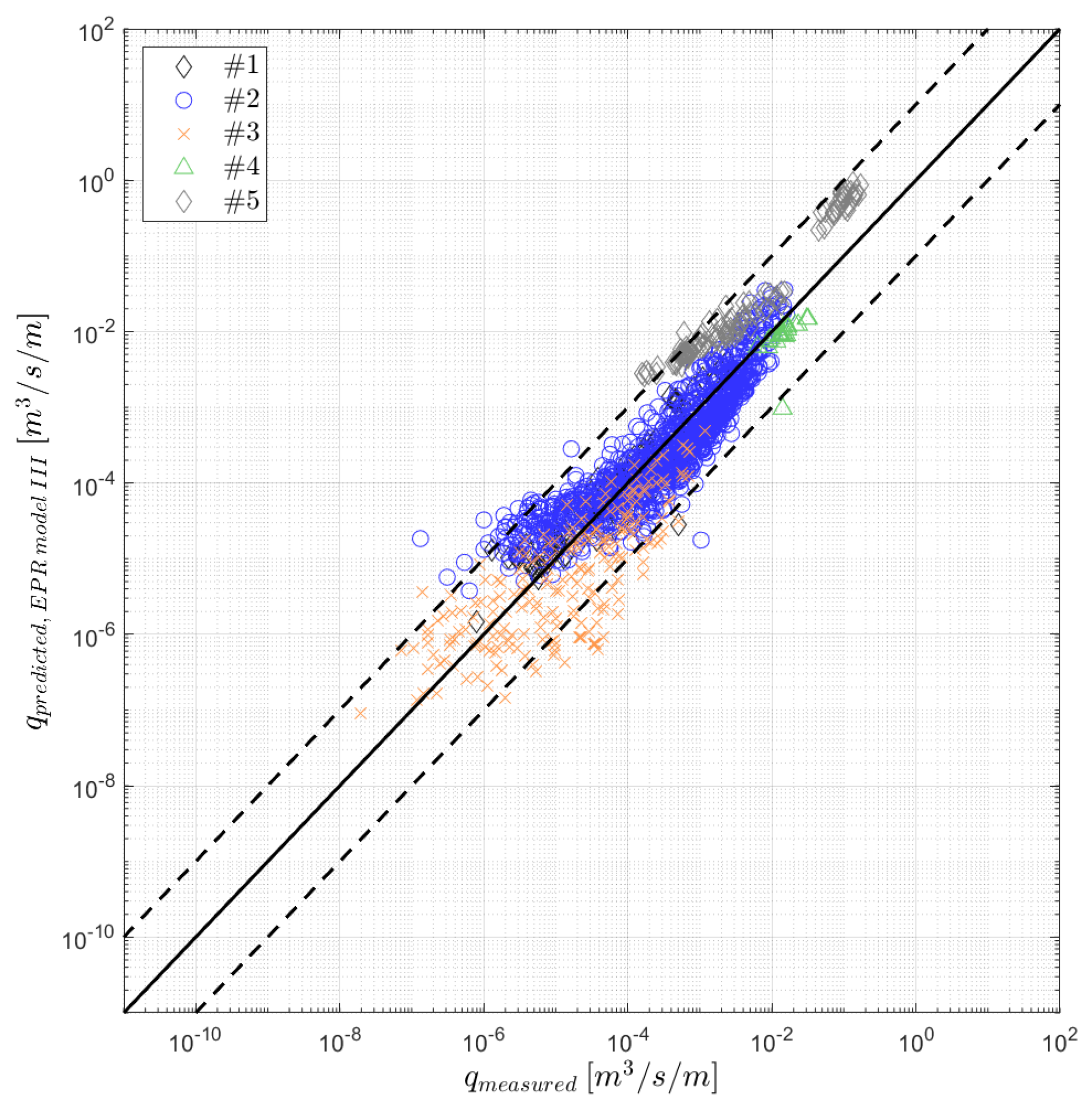
| III | 0.75 | 0.17 | 0.74 | 0.17 | |
| IV | 0.70 | 0.20 | 0.70 | 0.20 | |
| V | 0.71 | 0.20 | 0.71 | 0.19 | |
| VI | 0.73 | 0.18 | 0.74 | 0.18 | |
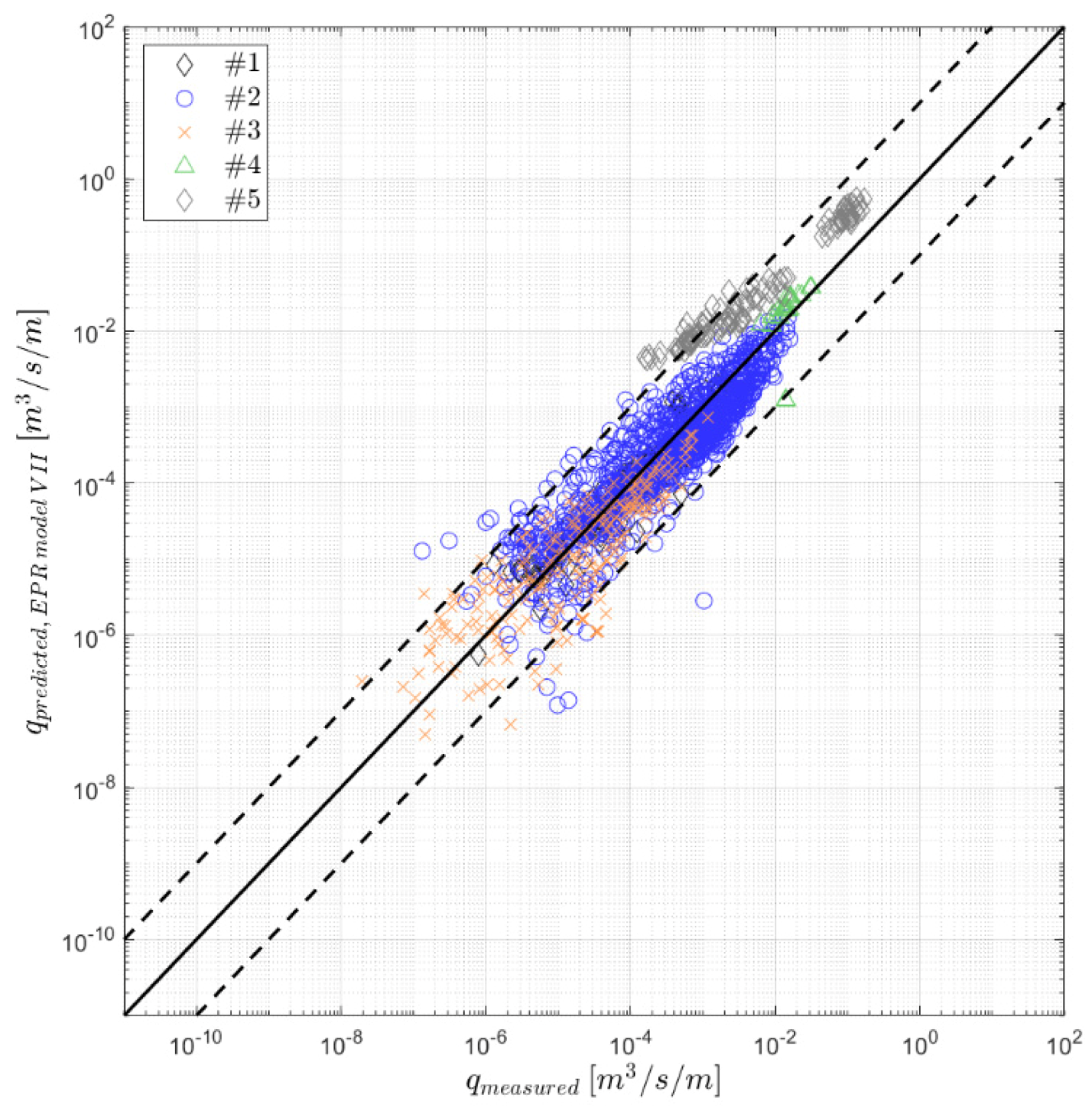
| VII | 0.76 | 0.16 | 0.74 | 0.16 | |
| VIII | 0.75 | 0.17 | 0.74 | 0.17 | |
| IX | 0.74 | 0.16 | 0.74 | 0.16 | |
| X | 0.76 | 0.15 | 0.76 | 0.16 | |
| Model # | GEO | GSD | qpred/qEXP | |
|---|---|---|---|---|
| μ − 1.64σ | μ + 1.64σ | |||
| I | 1.00 | 3.40 | 0.18 | 5.58 |
| II | 1.15 | 3.60 | 0.19 | 6.77 |
| III | 0.99 | 3.08 | 0.20 | 5.01 |
| IV | 1.00 | 3.38 | 0.18 | 5.53 |
| V | 1.00 | 3.29 | 0.19 | 5.39 |
| VI | 0.99 | 3.14 | 0.19 | 5.10 |
| VII | 0.99 | 2.98 | 0.20 | 4.84 |
| VIII | 0.85 | 3.00 | 0.17 | 4.18 |
| IX | 0.93 | 3.28 | 0.17 | 5.00 |
| X | 0.89 | 3.11 | 0.17 | 4.54 |
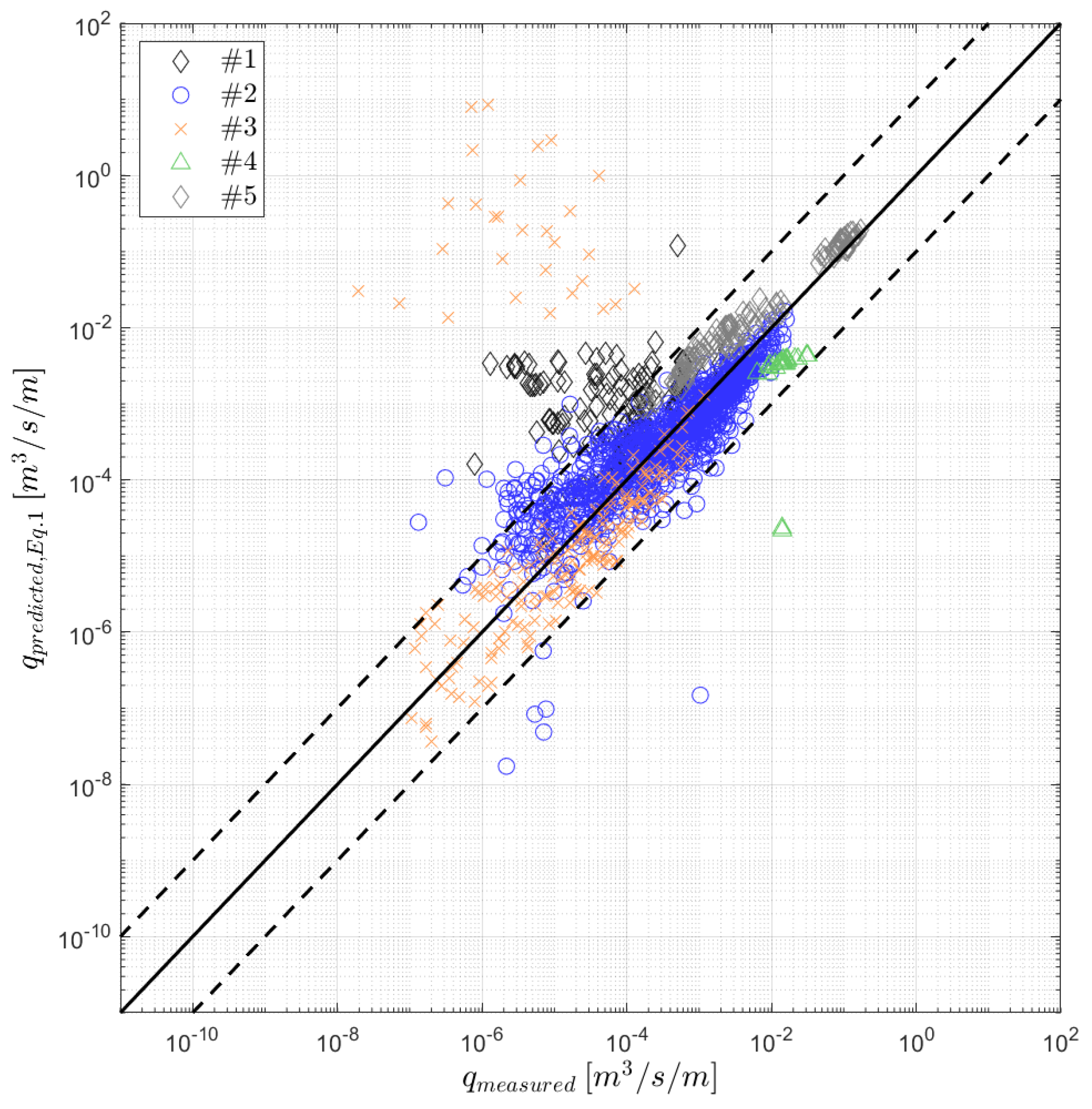
| Equation (1) | 1.59 | 8.03 | 0.12 | 20.94 |
| Equation (6) | 0.96 | 24.55 | 0.02 | 38.65 |
© 2020 by the authors. Licensee MDPI, Basel, Switzerland. This article is an open access article distributed under the terms and conditions of the Creative Commons Attribution (CC BY) license (http://creativecommons.org/licenses/by/4.0/).
Share and Cite
Altomare, C.; Laucelli, D.B.; Mase, H.; Gironella, X. Determination of Semi-Empirical Models for Mean Wave Overtopping Using an Evolutionary Polynomial Paradigm. J. Mar. Sci. Eng. 2020, 8, 570. https://doi.org/10.3390/jmse8080570
Altomare C, Laucelli DB, Mase H, Gironella X. Determination of Semi-Empirical Models for Mean Wave Overtopping Using an Evolutionary Polynomial Paradigm. Journal of Marine Science and Engineering. 2020; 8(8):570. https://doi.org/10.3390/jmse8080570
Chicago/Turabian StyleAltomare, Corrado, Daniele B. Laucelli, Hajime Mase, and Xavi Gironella. 2020. "Determination of Semi-Empirical Models for Mean Wave Overtopping Using an Evolutionary Polynomial Paradigm" Journal of Marine Science and Engineering 8, no. 8: 570. https://doi.org/10.3390/jmse8080570