

Comparison between Genetic Programming and Dynamic Models for Compact Electrohydraulic Actuators

Mechanical Engineering Department, Yonsei University, Seoul 03722, Korea
*
Author to whom correspondence should be addressed.
Machines 2022, 10(10), 961; https://doi.org/10.3390/machines10100961
Submission received: 19 September 2022
/
Revised: 14 October 2022
/
Accepted: 18 October 2022
/
Published: 21 October 2022
(This article belongs to the Special Issue Advanced Control of Electro-Hydraulic Systems in Industrial Area)
Abstract
:A compact electrohydraulic actuator (C-EHA) is an innovative hydraulic system with a wide range of applications, particularly in automation, robotics, and aerospace. The actuator provides the benefits of hydraulics without the expense and space requirements of full-sized hydraulic systems and in a much cleaner manner. However, this actuator is associated with some disadvantages, such as a high level of nonlinearity, uncertainty, and a lack of studies. The development of a robust controller requires a thorough understanding of the system behavior as well as an accurate dynamic model of the system; however, finding an accurate dynamic model of a system is not always straightforward, and it is considered a significant challenge for engineers, particularly for a C-EHA because the critical parameters inside cannot be accessed. Our research aims to evaluate and confirm the ability of genetic programming (GP) to model a nonlinear system for a C-EHA. In our paper, we present and develop a GP model for the C-EHA system. Furthermore, our study presents a dynamic model of the system for comparison with the GP model. As a result, by using this actuator in the 1-DOF arm system and conducting experiments, we confirmed that the GP model has a better performance with less positional error compared with the proposed dynamic model. The model can be used to conduct further studies, such as designing controllers or system simulations.
1. Introduction
Hydraulic actuators are among the most common in heavy industries. These actuation systems can provide a high amount of force while consuming a minimum amount of energy. However, most of these actuation systems are composed of a number of components that may impose limitations on the system. As a result, these types of actuators might be very difficult to use in applications where space, cleanliness, and weight are limited, such as in robotics and aerospace. A compact electrohydraulic actuator (C-EHA), which offers a number of advantages over conventional hydraulic actuators, has been developed to overcome this issue. Figure 1 shows a commercial type of this actuator. These actuators are significantly smaller and lighter compared with conventional hydraulic actuators, can run on battery power, are isolated, very clean, plug-and-play, and can be integrated into a wide range of systems. These characteristics distinguish this actuator and open up a broad variety of applications for it, particularly in positioning systems and robotics applications where high force is required in a limited space. Despite this product being well developed and already commercially available, engineers continue to improve the control system’s performance because these actuators are associated with a high level of non-linearity and uncertainty. Having an accurate model of the system could help improve tracking accuracy and enhance control performance, especially for model-based controllers [1].
The dynamic modeling approach is considered the most popular method of determining the system’s model. Modeling the system using physical rules offers its own set of benefits and provides engineers with a unique perspective on the system’s features. However, this strategy requires an extensive understanding of the system, which may not always be feasible when dealing with highly complex nonlinear systems, specifically hydraulic systems [2]. A variety of linear and nonlinear controllers have been well developed over the past few decades to more precisely control the conventional type of electrohydraulic actuators [3,4,5,6]. Most of these systems monitor and measure critical internal parameters, such as oil pressure and flow rate, during the actuator’s operation. These parameters can be utilized to considerably increase the controller’s precision and performance. Moreover, a standard controlled valve has been used to control most of these actuators’ cylinder rods. However, no such components to control the output of an C-EHA exist, which are also known as pump-controlled hydraulic or electrohydrostatic systems, or self-contained electrohydraulic cylinder drives (Figure 2). Because these actuators rely solely on the pump motor’s speed as input, it is difficult to determine an accurate dynamic model for the control system because oil pressure and flow rate are not accessible to measure in C-EHA systems.
This type of actuator has been the subject of several studies over the past decade with the aim of improving their characteristics, modeling, and identification, or developing higher-precision controllers. The following are some highlights from previous studies. Hagen et al. listed various types of internal structures for valveless types of actuators [7]. Ling et al. conducted a study on identifying the system and improving the accuracy of an EHA’s position-tracking system. The authors applied stimulus–response data and implemented system identification processes without applying physics laws for modeling, resulting in a linear model for the nonlinear system [8]. Nie et al. developed an extended-state-observer-based backstepping control system for underwater electrohydrostatic actuators [9]. Martin and Louis developed an electrohydrostatic actuator model; however, they only made simulations and did not compare the results with the actual actuator [10].
The some of research in the area of electrohydrostatic actuators is focused on controlled-valved actuators; valveless actuators have not received significant attention. Even though there have been some significant achievements in these studies, finding an accurate model of the system remains a challenge. As previously mentioned, measuring hydraulic actuator internal parameters such as oil pressure or flow rate can significantly increase the accuracy of the model and control. Due to the fact that these parameters are not accessible in this type of isolated system, the only parameter that can be measured is the pump speed. Therefore, developing an accurate model of the system is still considered a challenge for researchers.
Alternatively, artificial intelligence techniques can be utilized to facilitate the development of new modeling techniques without requiring the accurate dynamical models of various systems [11,12,13], specially an EHA [14,15]. Genetic programming (GP), an extension of genetic algorithms (GA), is a well-known solution for nonlinear problems. It is an optimization method that can be applied to optimize complex systems with nonlinear structures, as well as to present systems and their parameters [16]. GP provides a number of benefits, such as the possibility of utilizing system pre-knowledge to prepare a better initial candidate solution that could help to achieve better results [17]. GP has numerous applications in engineering, and it can be applied to the design and identification of various systems. For example, Santos utilized GP to identify a nonlinear model for an experimental ball-and-tube system [18]. Recently, Raibaudo and his team implemented GP on an experimental setup to optimize unsteady feedback controllers. The GP method also has additional applications in engineering and non-engineering fields (see [19,20,21,22]).
A primary objective of our research is to examine the effectiveness of using GP methods to develop an accurate model for a case study of a commercial type of C-EHA (Figure 1). We investigated a GP model that was proposed and reported in a previous paper, and we evaluated the accuracy and performance of this method [23]. Our study develops an appropriate dynamic mode for comparison. We applied the same input command to both dynamic and GP models, as well to a real actuator system. We performed a comparison of the position-tracking error data between the two models to check which has better accuracy.
An introduction to the C-EHA is provided in Section 2, followed by details on the development of a proper dynamic model. Section 3 briefly describes the GP method and the parameter settings developed in the previous paper, which we used in our study to model the compact electrohydraulic actuator. The experiment and final results for both the GP and dynamic models are presented and discussed in Section 4. The final section concludes our study.
2. Dynamic Modeling
2.1. Compact Electrohydraulic Actuator (C-EHA)
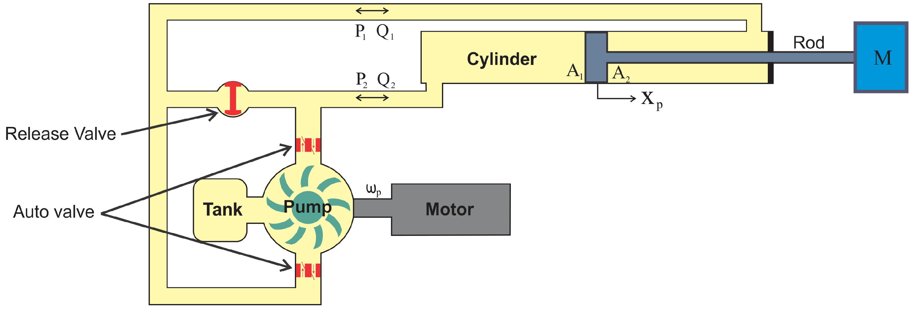
C-EHAs have a broad range of applications, particularly in automation and robotics, due to their unique features. In contrast to conventional actuators, this actuator does not use an actuated valve to control the amount of oil and, consequently, pressure on the piston sides. Instead, automatic valves, which control the flow of oil based on the rational direction of the pump, are integrated with the system. C-EHA technology simply connects two ports of a bi-directional gear pump to either side of a piston, along with a small oil reservoir as a means of generating an initial pressure. As a result of a motor driving the gear pump, the piston moves in either direction. Figure 3 shows that this actuator’s motor rotates the gear pump in one direction to pressurize the hydraulic fluid and extend the cylinder. Fluid is drawn from both the small reservoir inside the actuator and the cylinder’s head side as the auto-valves open, resulting in the actuator rod’s extension. The motor runs in the other direction during the retraction phase, reversing the operation and returning the fluid to the piston’s opposite side. The leakage is assumed to be negligible because of the system’s isolation and its inability to measure any internal leakage. The motion equation for this actuator can be derived using the continuity equation shown in (1) following the assumption that oil is not compressible [24,25].
where , , and are the flow rate, cylinder pressure, and cylinder volume, respectively. is defined as the effective bulk modulus of oil. The cylinder volume can be rewritten as in (2), where is the cylinder’s initial volume, is the piston position, and is the piston’s cross-section area.
The difference in pressure between the piston’s two sides generates external force. Equation (4) describes this external force in the presence of friction between the cylinder and piston.
As previously mentioned, the inside pressure value is unavailable for measurement. Thus, we can consider the derivative of (4) as follows.
The flow rates and are circulated by the internal gear pump, described as follows, where is the pump’s volumetric capacity and is the pump’s rotational speed.
The generated force’s final equation can be expressed as (7).
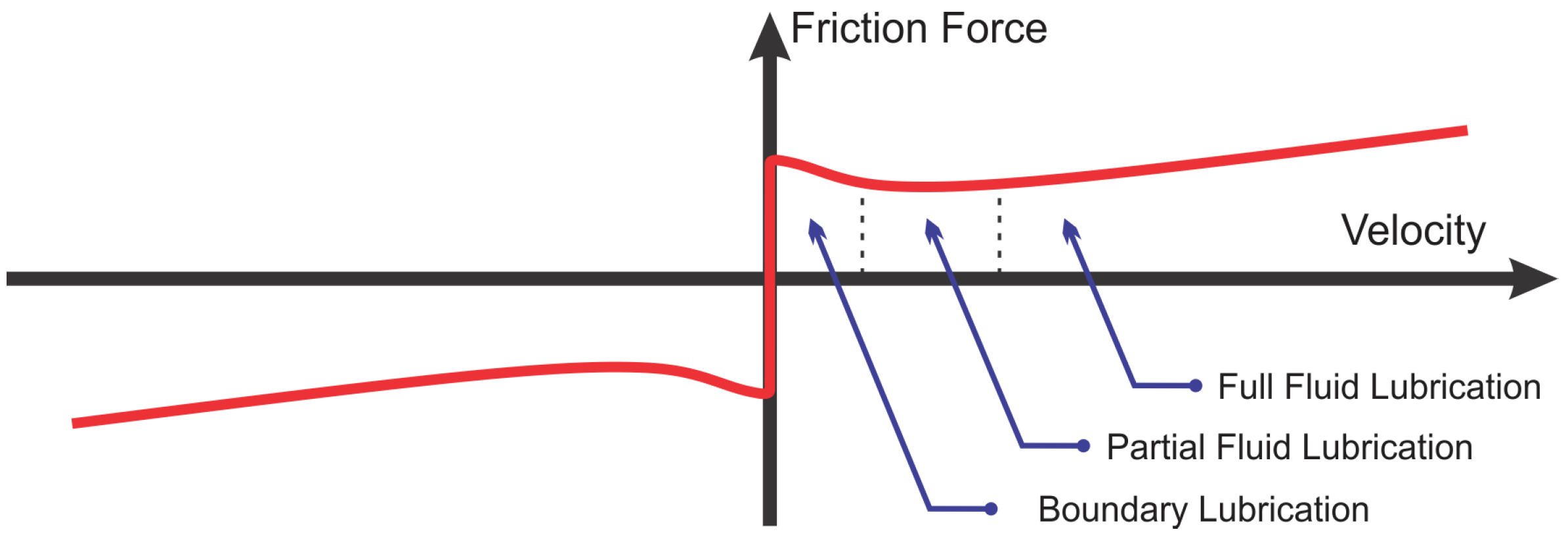
Stribeck effects are applied to determine the C-EHA’s friction model. Figure 4 shows the Stribeck effect for the viscus friction force as a function of velocity. Contact surfaces can have different friction forces depending on their velocities. There are four major regions; steady-state velocity, boundary lubrication, and partial fluid and full fluid lubrication. The friction model and its derivatives can be defined by (8) and (9), respectively [26].
where , , and are the coefficients of kinetic, static, and viscous frictions, respectively, and is the Stribeck velocity. We can determine these unknown parameters by performing specific tests on the actuator. Section 4.1 provides a detailed explanation of this procedure.
2.2. Equation of Motion for Arm Manipulator
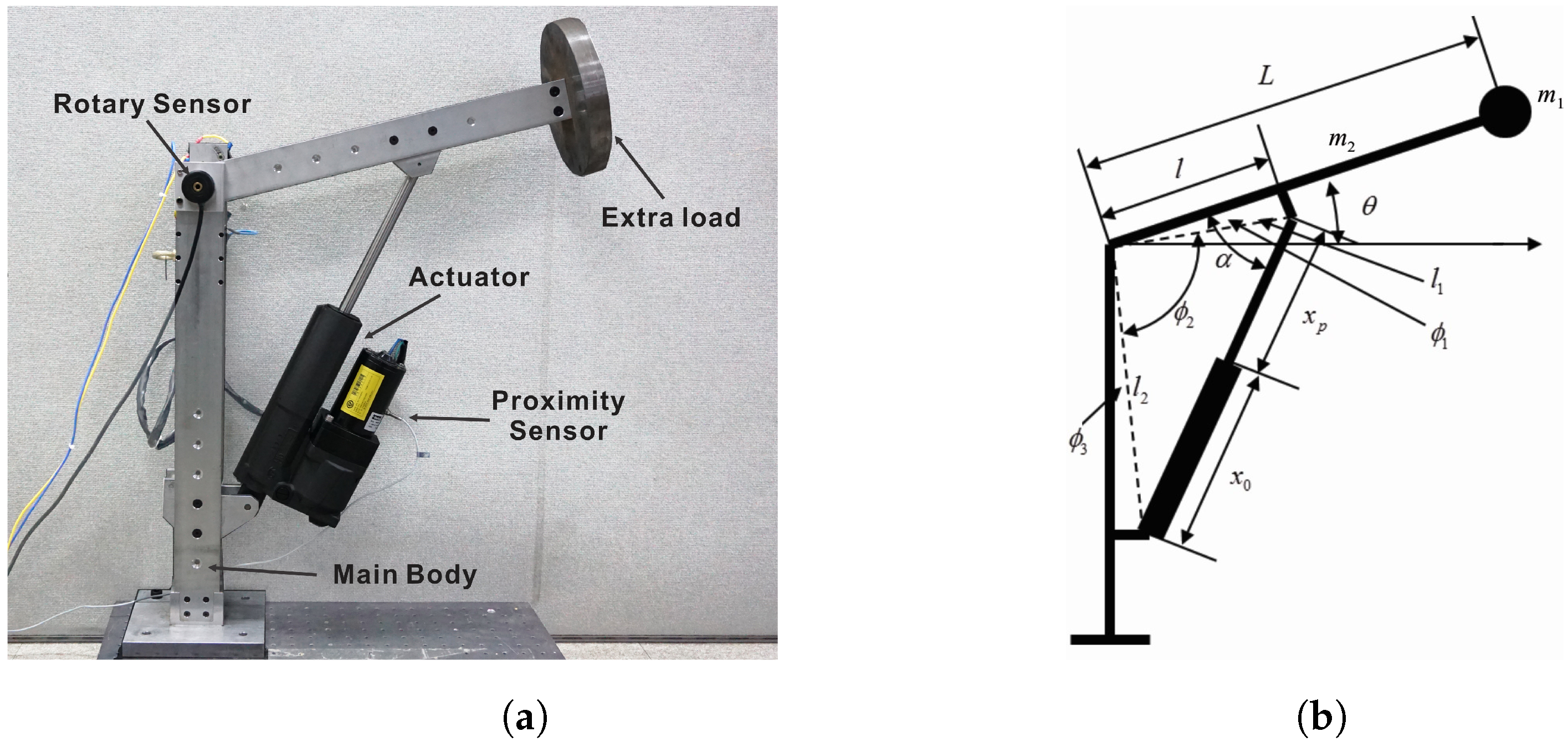
Figure 5a shows a one-DOF arm manipulator that we developed to provide the experimental datasets. This arm is equipped with the commercial-type C-EHA made by the Parker Hannifin Company with a maximum payload of (Figure 1).Both mounting sides of the C-EHA can be easily adjusted in this setup. A strong bolt is also used to attach the weight as an external load to the head of the arm. Weights of different sizes are provided, which can be easily changed or even installed together using longer bolts. Section 4 shows the results of a number of experiments we conducted to provide training and validation datasets for the GP model and find friction parameters for the dynamic models. We used these data to demonstrate the proposed models’ effectiveness and accuracy.
Here, we present the motion equation for the arm manipulator. We chose to apply the Lagrange method to this system to find the model. Based on the parameters defined in Figure 5b, (10) and (11) present the system’s kinematic and potential energy equations, respectively.
Lagrange’s method is described as follows
where represents the applied torque at the rotational joint. The relation between the external force and torque generated by the hydraulic actuator can be defined as follows:
3. Genetic Programming and Its Application for Hydraulic Actuator Problem
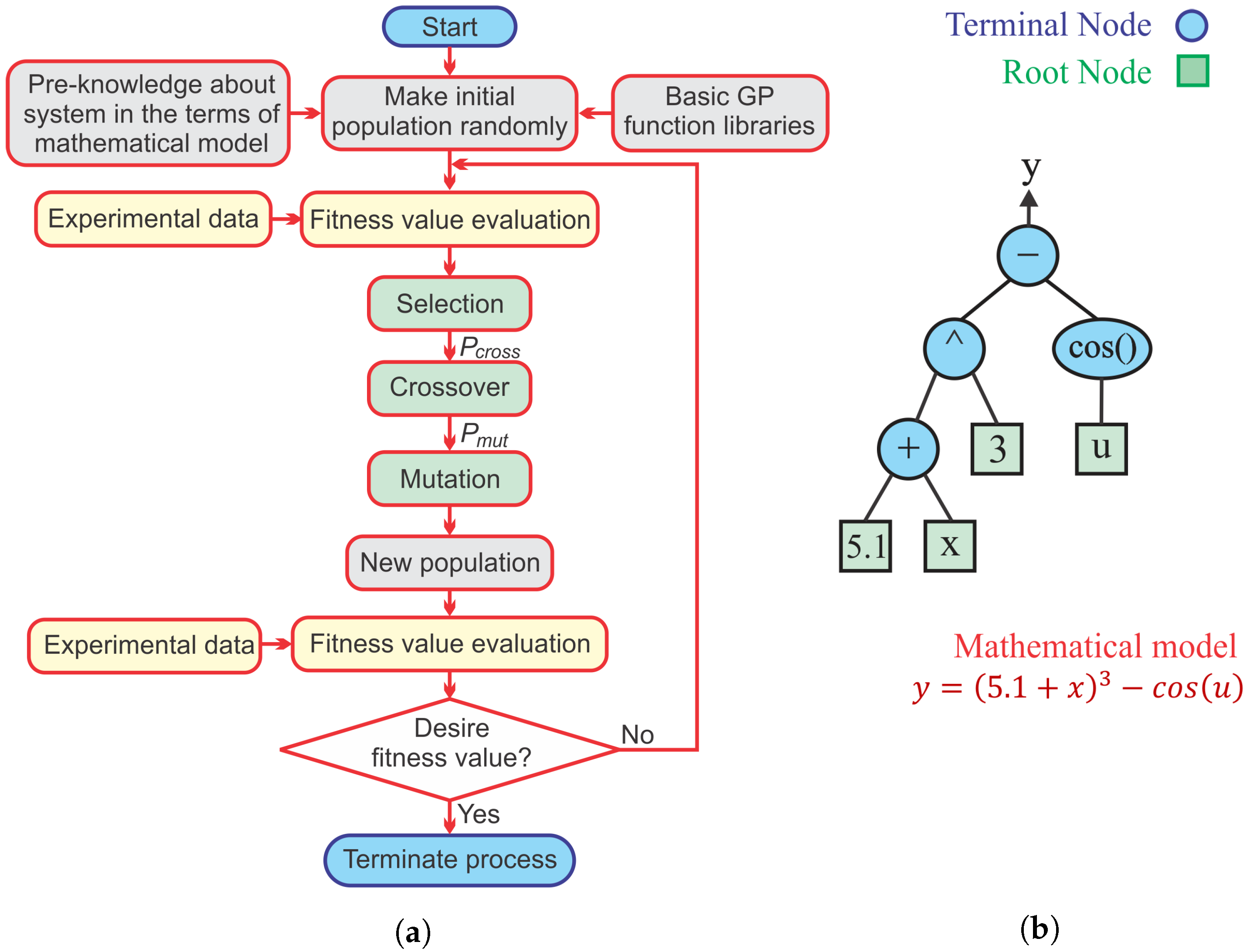
Genetic programming is considered an extension of genetic algorithms. Generally, genetic programming refers to an automated method of generating computer programs that carefully solve specific problems by the principle of natural selection. GP was created using evolutionary algorithms and was first developed by Barricelli to simulate evolution [27]. Later, Rechenberg used GP in the early 1970s to solve more complex engineering problems through evolution strategies. Nicholas Cramer made the first “tree-based” genetic programming declaration [28]; furthermore, John Koza played a key role in the development of GP and its application to a number of different situations [29]. The flowchart in Figure 6a illustrates a general GP procedure. The initial populations are made based on pre-knowledge of the system and basic algebra operations. A fitness function is used to evaluate each candidate solution based on the available training-set data, which is obtained from experiments. As each candidate solution undergoes GP operations, their fitness values impact their chances of survival. Good candidate solutions can be improved with each successive generation and, ultimately, the best result can be achieved after many generations. The final model’s validation can be conducted using the validation-set data obtained from the experiments. In our study, we used previously proposed GP model structures and parameters, which are briefly discussed as follows [23].
3.1. Encoding and Initial Population
Figure 6 shows all the individuals are encoded as a tree structure in a mathematical model. Terminal (basic algebra operations and subfunctions) and root nodes (constant numbers and inputs) exist in every structure. GP individuals do not have a fixed length, and they may change from generation to generation. Randomly selecting initial candidates allows GP to generate a wide range of candidate solutions [16]. However, C-EHA requires only one input command to increase the GP model’s accuracy, with the motor pump’s current speed as an input also being considered. Additionally, the arm’s current position is also added to the model as an input to obtain the arm’s absolute position. Considering these three inputs and one output as the next arm position, the GP model is considered a multi-input–single-output model (MISO). Considering the available functions and conditions, we assume that each node can have a maximum of two branches and a minimum of none. The candidate’s final value can then be calculated by using the input values and substituting them into the roots.
3.2. Function Library
Generally, function libraries can be imagined as pools containing functions and terminal sets for making initial population or mutation branches. The terminal set consists of statements, operations, basic algebra, and sub-functions while the root set is composed of the system inputs and constant numbers. Any prior knowledge of the system should also be considered for the initial population. Therefore, in addition to the basic algebraic and sinusoidal functions, the hyperbolic tangent function is also selected as part of the function library because it has similar properties to the friction model.
3.3. Fitness Function
Fitness functions are a type of objective function that measures how well a solution candidate performs in comparison with the actual data available. Several well-known fitness functions exist for GA and GP depending on the conditions [30]. We define fitness function in our study as the sum of squared errors between the model output and experimental data.
3.4. Operations
Similar to the GA method, the GP method uses three major operations to create the main components of the GP: selection, crossover, and mutation [31]. The selection process, such as roulette-wheel, tournament, ranking, and elitist selection, is the process in which candidates from one generation are selected according to the selection method and fitness values to generate new candidates for the next generation. Crossover refers to the process of combining two individuals (parents) to create new individuals (offspring). A mutation is a genetic operation that changes one part of an individual by using a randomly generated sub-tree. In each generation, after the selection operation, both crossover and mutation operations are usually partially applied to the candidates during the evaluation based on their probability factors. These factors might vary depending on the optimization. In our proposed GP model, in accordance with elitist selection theory, 25 percent of the population with the highest fitness values are directly passed down to the next generation in order to avoid the effects of crossover and mutation. The remainder of the population is then subjected to crossover and mutation with rates of 80% and 3%, respectively. We used the roulette-wheel method to select candidates for crossover and mutation operations. These operations may result in a longer or shorter tree structures because of the random selection of nodes for crossover and mutation. However, long structures pose some challenges to GP. Consequently, we defined a 20-node limit for individuals to avoid creating long tree structures. An operation that produces offspring with a length greater than the limitation is not acceptable, and the selected node should be changed again until the new tree structure length is less than the limitation.
3.5. Termination
Using termination rules, a genetic algorithm determines whether to continue searching for a better answer or to stop searching. The termination criterion is checked after each generation to determine whether the answer meets the criterion. Based on the problem conditions, there are many ways to define the criteria for termination. The most well-known criteria are generation number, fitness threshold, and fitness convergence [32]. We used all three criteria simultaneously in our study to determine termination during the GP generations.
4. Experiment, Result, and Discussion
Our research requires various experiments to be designed and performed in order to produce data sets. Three major experiment setups are designed and conducted as follows.
4.1. Friction Parameter Identification
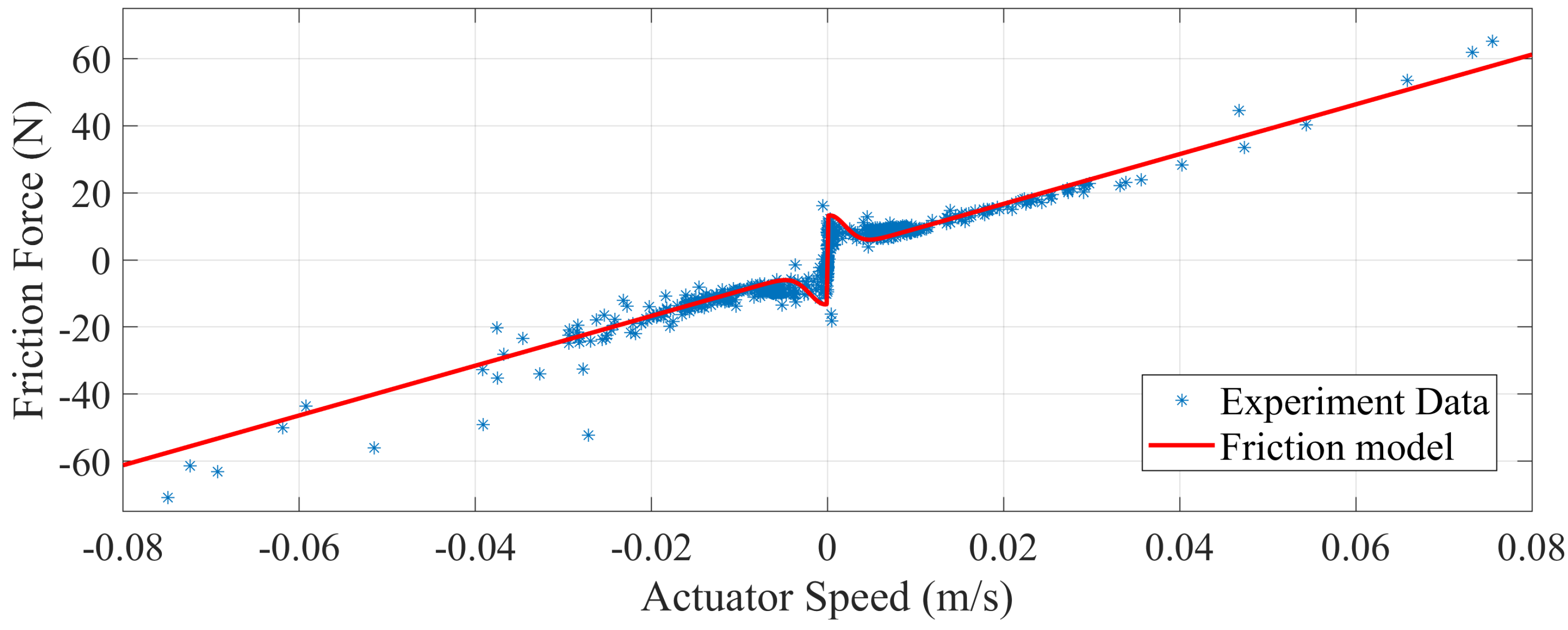
To find the unknown friction coefficients expressed in Equation (8) and check how much the friction term can affect the system response, it is essential to obtain the relation between the friction force and actuator speed. The first step in conducting such a test is to activate the manual release valve in the C-EHA to make a passive motion of the piston while the actuator is not in operation mode. Next, the system should be moved at a constant speed by applying controlled external force. We measured and recorded the external force and piston velocity for post-processing. The external load represents the amount of friction inside the actuator because it is not in operation. Figure 7 shows the results of a number of tests conducted at various speeds. We obtained the arm manipulator’s estimated friction parameters using Matlab curve-fitting toolbox and listed them in Table 1 along with other geometric parameters. Figure 7 shows the range of inner-friction force () is relatively smaller than the actuator maximum payload when it is in operation (). Friction terms can be neglected depending on the system and the model’s purpose. Nevertheless, we did not ignore them in our study.
4.2. GP Dataset
The GP method requires two sets of data for training and validation purposes. We conducted a large number of tests on the real system while measuring and recording inputs and outputs using a computer to create these datasets. The piston’s speed in this actuator is controlled exclusively by the pump speed, which is directly related to the motor input voltage. We conducted five sets of 80-s tests for GP training, as well as three sets for validation. A variety of frequencies and amplitudes are incorporated into input commands for creating datasets to ensure that all of the various actuator modes are stimulated (Figure 8).
4.3. Dynamic Model Validation
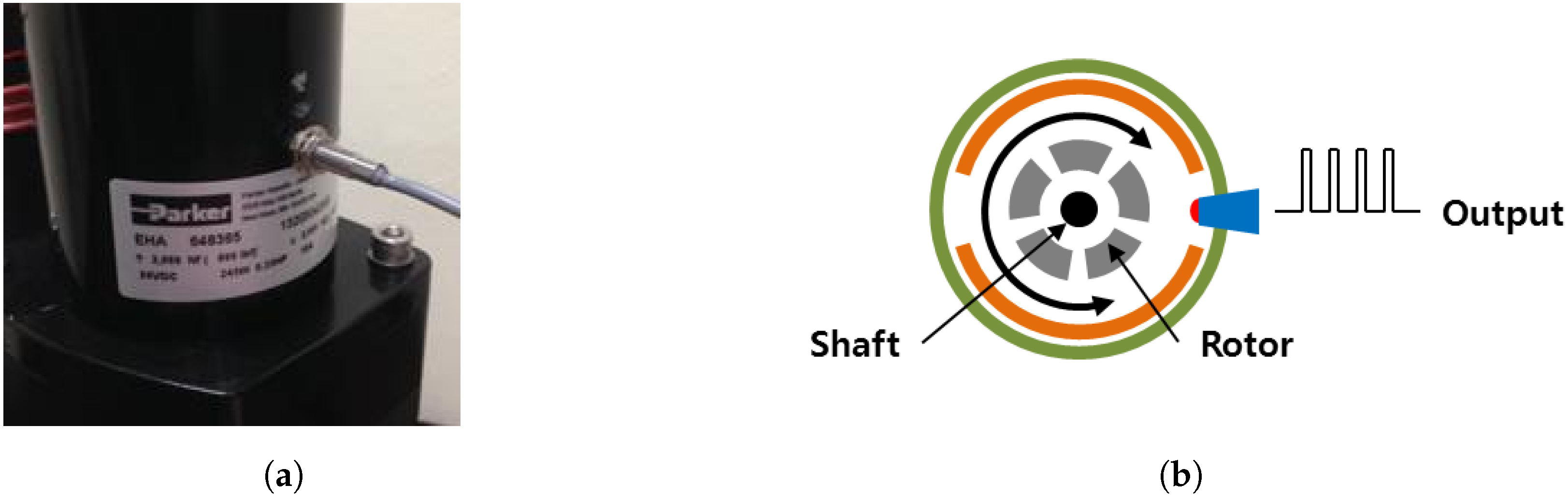
We implemented the same validation tests utilized for the GP model to validate our proposed dynamic system model. Furthermore, the results can be used to compare the performance of the two methods. However, the motor speed rather than motor voltage is required for dynamic models. We attached a proximity sensor to the motor side prior to conducting tests to determine motor speed (Figure 9). We conducted additional tests to provide a relationship between the motor voltage and speed. Figure 10 shows that this relation can be considered linear.
4.4. Results
We used the GP method to obtain a model of the system based on the training data set. The following Equation (17) represents the best answer found by the GP method:
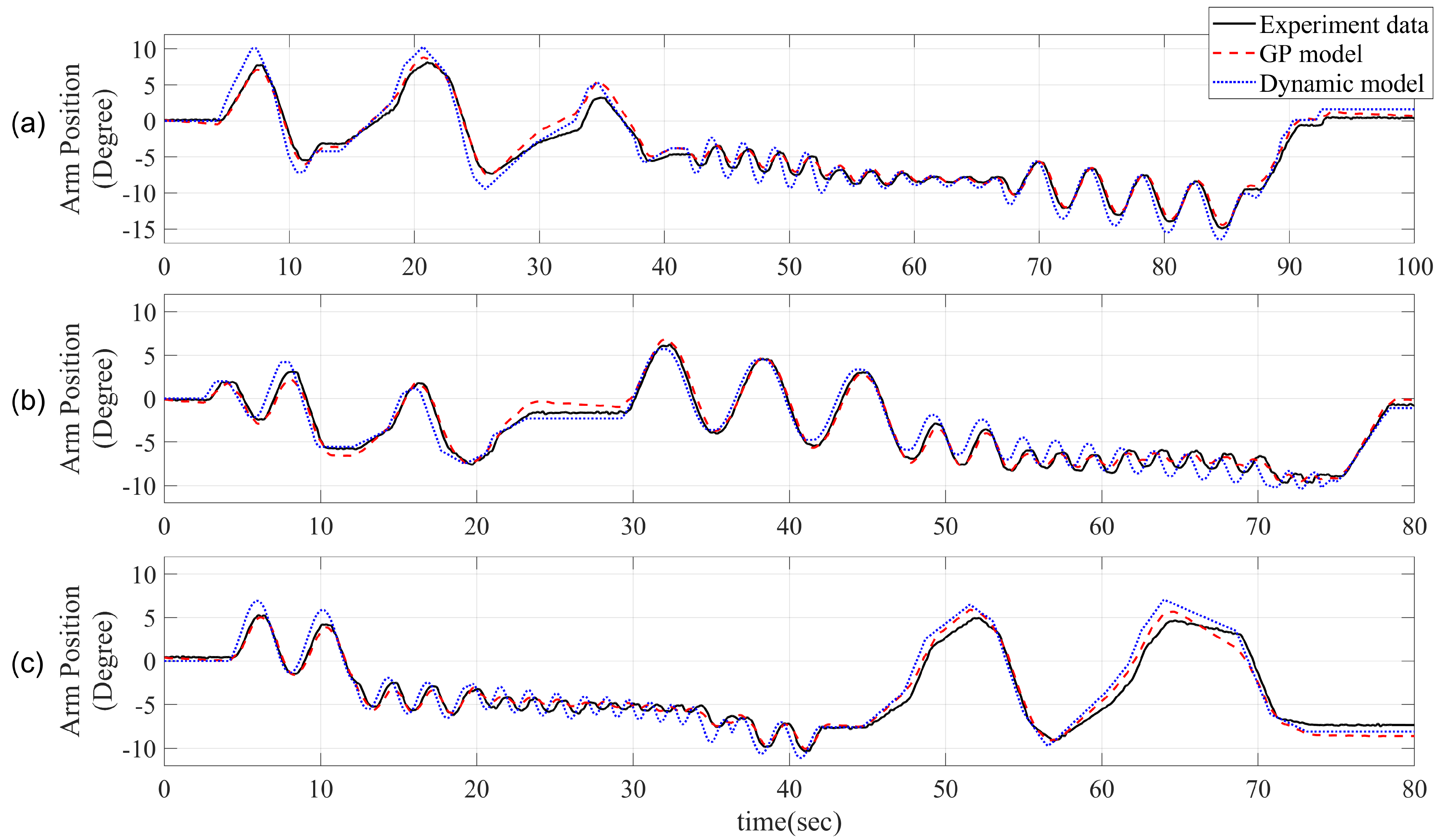
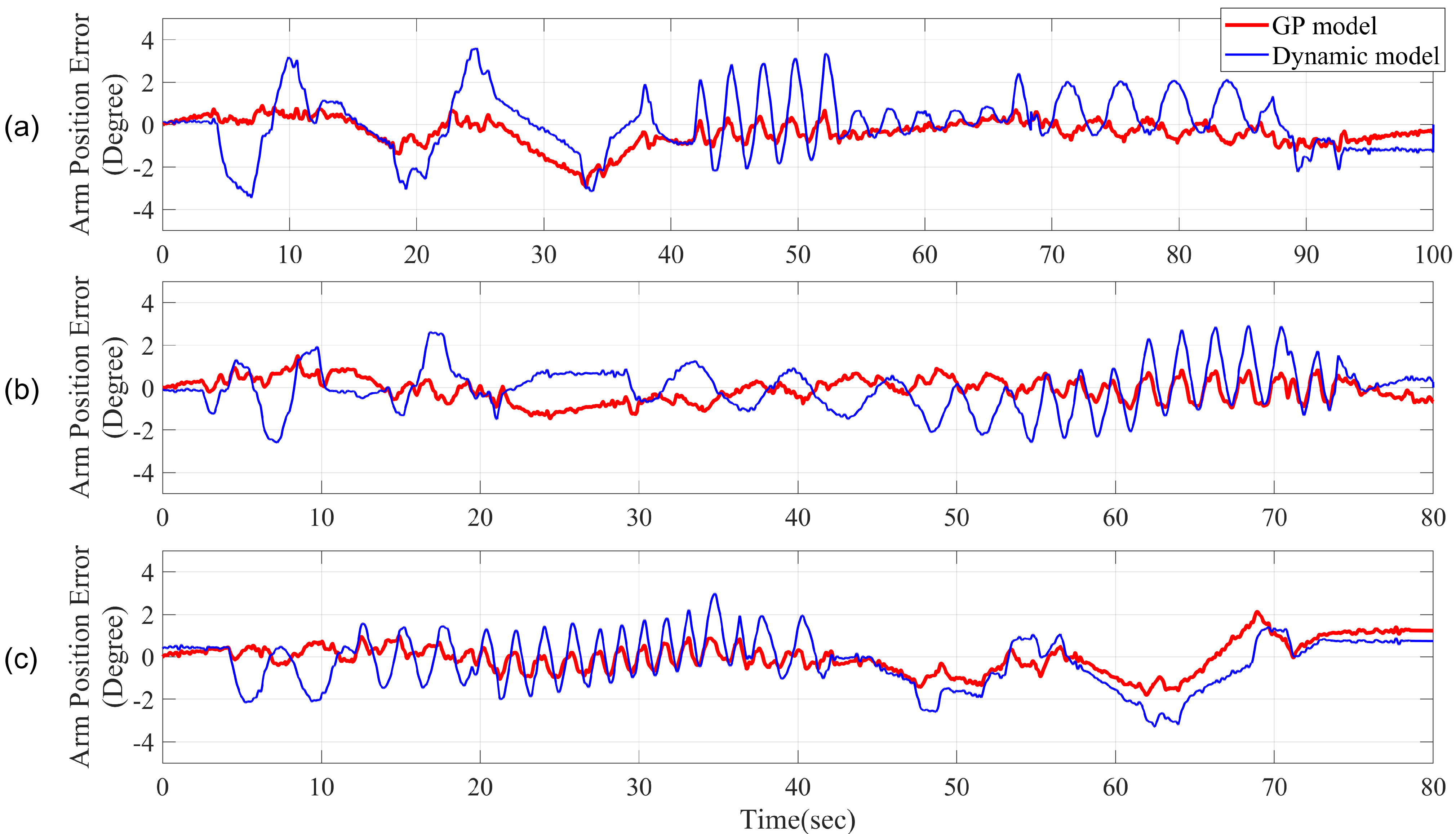
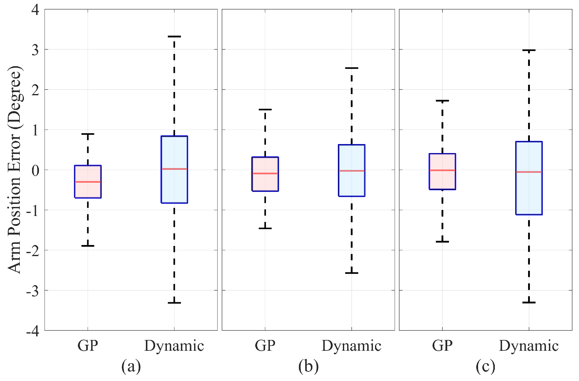
where, , , and represent the current motor position, the voltage input, and the motor velocity, respectively. In our study, each time step is 1 millisecond. This is followed by applying the three different validation input command sets to the dynamic and GP models, resulting in the arm angle and speed illustrated in Figure 11 and Figure 12, respectively. As can be seen in these figures, the GP model has slightly better accuracy in comparison to the dynamic model. Position accuracy is of greater concern in most C-EHA applications because C-EHA actuators operate at low speeds compared with other actuators. Therefore, for ease of comparision, the position error between these two models and experimental data presented in Figure 11 are calculated and presented in Figure 13. As can be seen in these figures, the GP model has slightly better accuracy in comparison to the dynamic model. This could be confirmed with the error bar presented in Figure 14. Moreover, the root mean square error (RMSE) of each dataset for each model is calculated by following equation;
where . The results in Table 2 confirm that the GP model has a slightly better performance in comparison with the dynamic method.
5. Conclusions
We employed two different modeling methods in our study to obtain a compact electrohydraulic actuator model and analyze its performance and accuracy. We developed a one-DOF arm with a payload to provide experimental data where all input and output can be measured and recorded by a computer. First, we created a dynamic actuator model along with a friction model for the system. Because the critical parameters, such as pressure or flow rate, are not accessible for measurements during the actuator’s operation, we need to be consider some assumptions that could reduce the dynamic model’s accuracy. We identified friction parameters through the specific experiment and curve fitting technique. Figure 8 shows that the friction-force contribution to the system response is considerably small regarding the payload rate; therefore, we consider it negligible. However, we decided to include it in the final model to keep the accuracy of the dynamic model as high as possible. We used the parameters of a previously developed GP model to obtain our model. We obtained various sets of training and validation data by utilizing an experimental setup. Finally, we employed both models to estimate the system’s response to the input command using a variety of validation datasets, as shown in Figure 11. The error of these two models is presented in Figure 12 and Figure 13 and Table 2. Our final results confirm that the GP model has a relatively effective performance, which could be used later for further simulations or improving control accuracy. Although it may be difficult to represent these GP models at a state–space level or to rewrite them as frequency responses, they can still be used for system simulations or in reference model controllers. More work can be performed in this field, and the exact practical applications of this model will be investigated in future works.
Author Contributions
Writing—original draft preparation, H.B.; writing—review and editing, S.J. and H.J.; review and editing, J.L.; supervision and project administration, H.Y. All authors have read and agreed to the published version of the manuscript.
Institutional Review Board Statement
Not applicable.
Informed Consent Statement
Not applicable.
Data Availability Statement
The data presented in this study are available on request from the corresponding author.
Conflicts of Interest
The authors declare no conflict of interest.
References
- Milecki, A.; Rybarczyk, D. Modelling of an Electrohydraulic Proportional Valve with a Synchronous Motor. Stroj. Vestn. J. Mech. Eng. 2015, 61, 517–522. [Google Scholar] [CrossRef]
- Detiček, E.; Kastrevc, M. Design of Lyapunov Based Nonlinear Position Control of Electrohydraulic Servo Systems. Stroj. Vestn. J. Mech. Eng. 2016, 62, 163–170. [Google Scholar] [CrossRef] [Green Version]
- Detiček, E.; Župerl, U. An Intelligent Electro-Hydraulic Servo Drive Positioning. Stroj. Vestn. J. Mech. Eng. 2011, 57, 394–404. [Google Scholar] [CrossRef]
- Ishak, N.; Julaihi, F.; Yusof, N.M.; Tajuddin, M.; Adnan, R. Load effect studies on ARX model parameters of vertical position Electro-Hydraulic Actuator. In Proceedings of the 2016 IEEE 12th International Colloquium on Signal Processing and Its Applications (CSPA), Melaka, Malaysia, 4–6 March 2016; pp. 301–304. [Google Scholar] [CrossRef]
- Shiralkar, A.; Kurode, S.; Gore, R.; Tamhane, B. Robust output feedback control of electro-hydraulic system. Int. J. Dyn. Control 2019, 7, 295–307. [Google Scholar] [CrossRef]
- Yousef, M.; El-Sanabawy, M.; Rabie, G.; Rateb, R. Modeling, simulation and controller design for a typical bent axis electrohydraulic servo motor. In Proceedings of the International Conference on Aerospace Sciences and Aviation Technology, Cairo, Egypt, 6–8 April 2021; Volume 19, pp. 1–14. [Google Scholar]
- Hagen, D.; Padovani, D.; Ebbesen, M.K. Study of a Self-Contained Electro-Hydraulic Cylinder Drive. In 2018 Global Fluid Power Society PhD Symposium (GFPS); IEEE: Piscataway, NJ, USA, 2018; pp. 1–7. [Google Scholar] [CrossRef]
- Ling, T.G.; Rahmat, M.F.; Husain, A.R. System identification and control of an Electro-Hydraulic Actuator system. In Proceedings of the 2012 IEEE 8th International Colloquium on Signal Processing and its Applications, Malacca, Malaysia, 23–25 March 2012; pp. 85–88. [Google Scholar] [CrossRef] [Green Version]
- Nie, Y.; Liu, J.; Lao, Z.; Chen, Z. Modeling and Extended State Observer-Based Backstepping Control of Underwater Electro Hydrostatic Actuator with Pressure Compensator and External Load. Electronics 2022, 11, 1286. [Google Scholar] [CrossRef]
- Gendrin, M.; Dessaint, L. Multidomain high-detailed modeling of an electro-hydrostatic actuator and advanced position control. In Proceedings of the IECON 2012—38th Annual Conference on IEEE Industrial Electronics Society, Montreal, QC, Canada, 25–28 October 2012; pp. 5463–5470. [Google Scholar] [CrossRef]
- Chang, S.; Cho, S.G. An Intelligent Process to Estimate the Nonlinear Behaviors of an Elasto-Plastic Steel Coil Damper Using Artificial Neural Networks. Actuators 2022, 11, 9. [Google Scholar] [CrossRef]
- Jiangang, Y. Modelling and analysis of step response test for hydraulic automatic gauge control/Modeliranje in analiza odziva sistema samodejnega hidravlicnega krmiljenja debeline na stopnico. Stroj. Vestn.-J. Mech. Eng. 2015, 61, 115–124. [Google Scholar] [CrossRef]
- Cus, F.; Zuperl, U.; Kiker, E. A model-based system for the dynamic adjustment of cutting parameters during a milling process. Stroj. Vestn.-J. Mech. Eng. 2007, 53, 524–540. [Google Scholar]
- Nie, S.; Gao, J.; Ma, Z.; Yin, F.; Ji, H. An artificial neural network supported performance degradation modeling for electro-hydrostatic actuator. J. Braz. Soc. Mech. Sci. Eng. 2022, 44, 1–17. [Google Scholar] [CrossRef]
- Kim, H.M.; Park, S.H.; Lee, J.M.; Kim, J.S. A robust control of electro hydrostatic actuator using the adaptive back-stepping scheme and fuzzy neural networks. Int. J. Precis. Eng. Manuf. 2010, 44, 227–236. [Google Scholar] [CrossRef]
- Sette, S.; Boullart, L. Genetic programming: Principles and applications. Eng. Appl. Artif. Intell. 2001, 14, 727–736. [Google Scholar] [CrossRef]
- Gray, G.J.; Murray-Smith, D.J.; Li, Y.; Sharman, K.C.; Weinbrenner, T. Nonlinear model structure identification using genetic programming. Control Eng. Pract. 1998, 6, 1341–1352. [Google Scholar] [CrossRef]
- dos Santos Coelho, L.; Pessôa, M.W. Nonlinear model identification of an experimental ball-and-tube system using a genetic programming approach. Mech. Syst. Signal Process. 2009, 23, 1434–1446. [Google Scholar] [CrossRef]
- Beligiannis, G.N.; Skarlas, L.V.; Likothanassis, S.D.; Perdikouri, K.G. Nonlinear model structure identification of complex biomedical data using a genetic-programming-based technique. IEEE Trans. Instrum. Meas. 2005, 54, 2184–2190. [Google Scholar] [CrossRef]
- Zhang, L.; Jack, L.B.; Nandi, A.K. Fault detection using genetic programming. Mech. Syst. Signal Process. 2005, 19, 271–289. [Google Scholar] [CrossRef]
- Yeun, Y.S.; Suh, J.C.; Yang, Y.S. Function approximations by superimposing genetic programming trees: With applications to engineering problems. Inf. Sci. 2000, 122, 259–280. [Google Scholar] [CrossRef]
- Pérez, J.L.; Cladera, A.; Rabu nal, J.R.; Martínez-Abella, F. Optimization of existing equations using a new Genetic Programming algorithm: Application to the shear strength of reinforced concrete beams. Adv. Eng. Softw. 2012, 50, 82–96. [Google Scholar] [CrossRef]
- Bamshad, H.; Jegal, M.; Yang, H.S. System Identification Using Genetic Programming for Electro-Hydraulic Actuator. J. Autom. Control Eng. 2015, 3, 457–462. [Google Scholar] [CrossRef]
- Márton, L.; Fodor, S.; Sepehri, N. A practical method for friction identification in hydraulic actuators. Mechatronics 2011, 21, 350–356. [Google Scholar] [CrossRef]
- Kiani-Oshtorjani, M.; Ustinov, S.; Handroos, H.; Jalali, P.; Mikkola, A. Real-Time Simulation of Fluid Power Systems Containing Small Oil Volumes, Using the Method of Multiple Scales. IEEE Access 2020, 8, 196940–196950. [Google Scholar] [CrossRef]
- Armstrong-Helouvry, B. Control of Machines with Friction; Springer Science & Business Media: Berlin/Heidelberg, Germany, 2012; Volume 128. [Google Scholar]
- Barricelli, N.A. Numerical testing of evolution theories. Acta Biotheor. 1962, 16, 69–98. [Google Scholar] [CrossRef]
- Cramer, N.L. A representation for the adaptive generation of simple sequential programs. In Proceedings of the First International Conference on Genetic Algorithms, Pittsburgh, PA, USA, 24–26 July 1985; pp. 183–187. [Google Scholar]
- Angeline, P.J. Genetic Programming: On the Programming of Computers by Means of Natural Selection; MIT Press: Cambridge, MA, USA, 1992; ISBN 0-262-11170-5. [Google Scholar]
- Fan, W.; Fox, E.A.; Pathak, P.; Wu, H. The effects of fitness functions on genetic programming-based ranking discovery for Web search. J. Am. Soc. Inf. Sci. Technol. 2004, 55, 628–636. [Google Scholar] [CrossRef]
- Deb, K. An introduction to genetic algorithms. Sadhana 1999, 24, 293–315. [Google Scholar] [CrossRef]
- Madar, J.; Abonyi, J.; Szeifert, F. Genetic programming for system identification. In Proceedings of the Intelligent Systems Design and Applications (ISDA 2004) Conference, Budapest, Hungary, 26–28 August 2004. [Google Scholar]
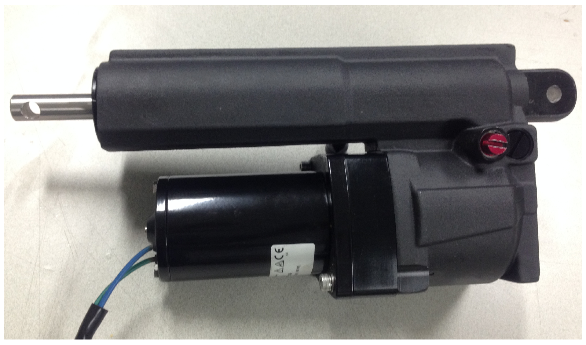
Figure 1.
Commercial C-EHA made by Parker Hannifin company (Cleveland, OH, USA). (EHA 648365, SN:1320504338, 24VDC, max speed: 0.08 m/s, max payload: 2669 Nf/600 lbf).
Figure 1.
Commercial C-EHA made by Parker Hannifin company (Cleveland, OH, USA). (EHA 648365, SN:1320504338, 24VDC, max speed: 0.08 m/s, max payload: 2669 Nf/600 lbf).

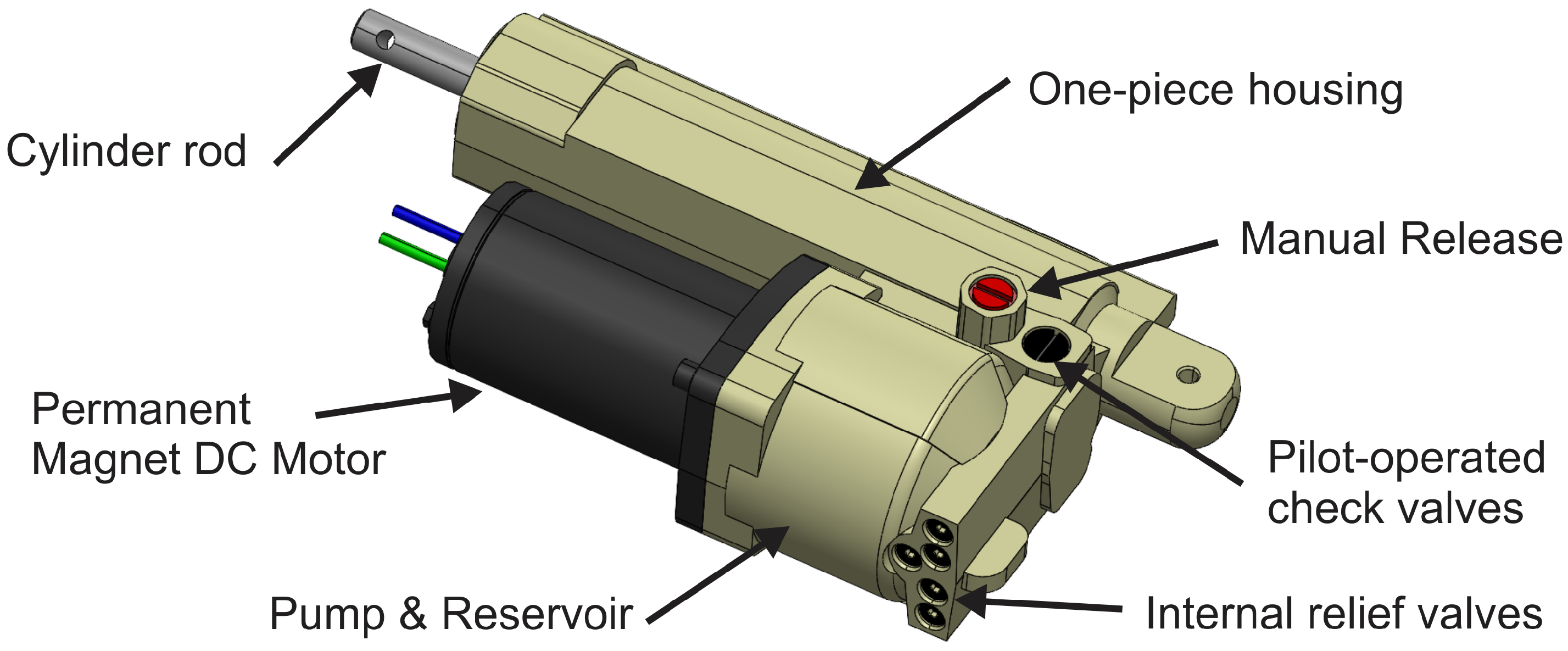
Figure 2.
3D model of C-EHA and main components.

Figure 3.
Simplified C-EHA mechanism.

Figure 4.
Stribeck effect model.

Figure 5.
One-DOF arm manipulator developed as experiment setup: (a) experimental setup, (b) schematic diagram.
Figure 5.
One-DOF arm manipulator developed as experiment setup: (a) experimental setup, (b) schematic diagram.

Figure 6.
Genetic programming (GP) structure: (a) flow chart, (b) tree structure example.

Figure 7.
Stribeck effect model found by experimental data.

Figure 8.
Random input commands to generate validation data sets: (a) Test Set 1, (b) Test Set 2, and (c) Test Set 3.
Figure 8.
Random input commands to generate validation data sets: (a) Test Set 1, (b) Test Set 2, and (c) Test Set 3.

Figure 9.
C-EHA motor encoder: (a) attached sensor, (a) working principle.

Figure 10.
Relationship between motor controller input command and motor velocity.

Figure 11.
Arm position obtained using experiment, GP model, and dynamic models for (a) first validation input command set, (b) second validation input command set, and (c) third validation input command set.
Figure 11.
Arm position obtained using experiment, GP model, and dynamic models for (a) first validation input command set, (b) second validation input command set, and (c) third validation input command set.

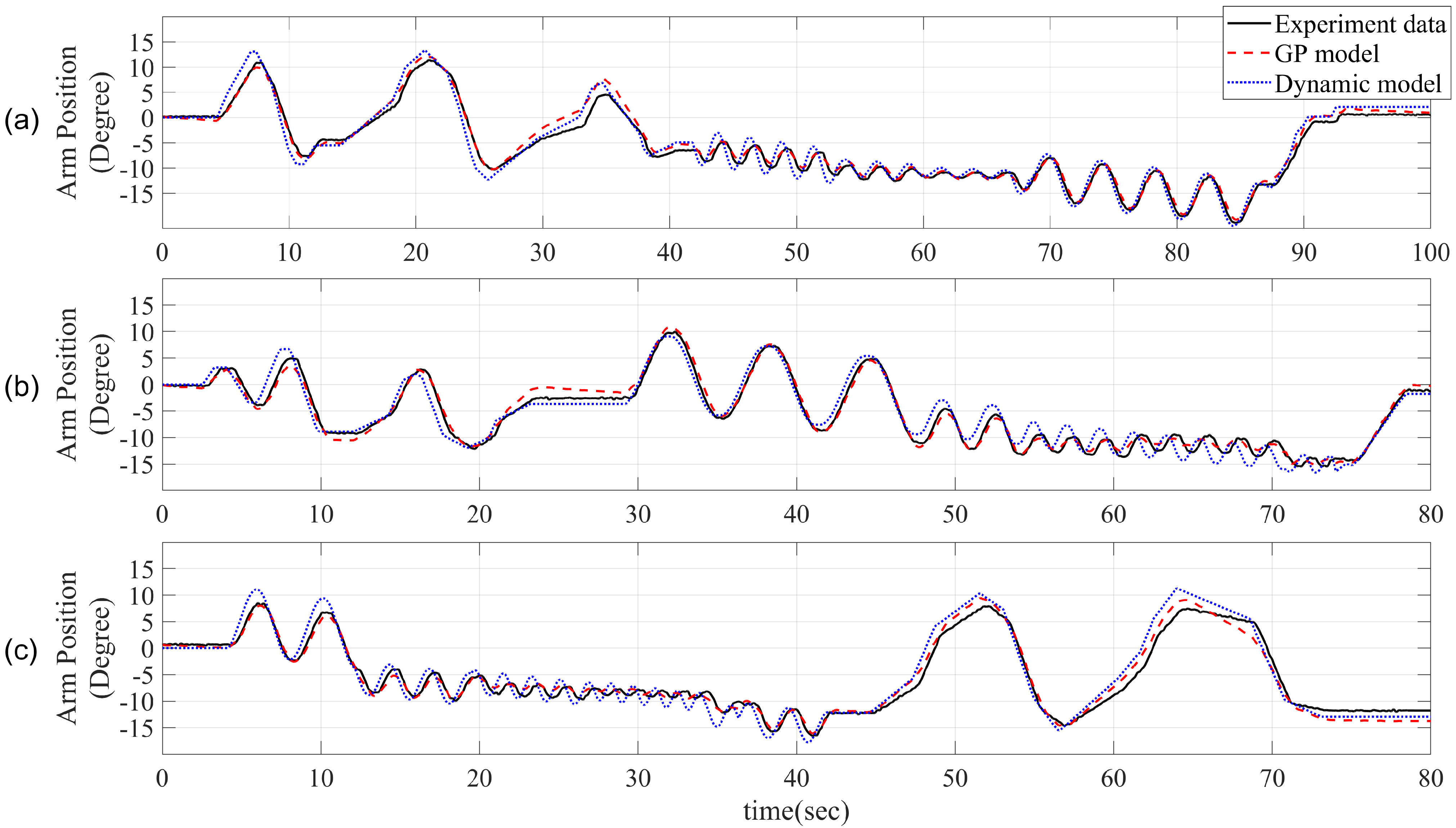
Figure 12.
Arm speed obtained using experiment, GP model, and dynamic models for (a) first validation input command set, (b) second validation input command set, and (c) third validation input command set.
Figure 12.
Arm speed obtained using experiment, GP model, and dynamic models for (a) first validation input command set, (b) second validation input command set, and (c) third validation input command set.

Figure 13.
Arm position error for two methods with respect to the experimental data, (a) first validation dataset, (b) second validation dataset, (c) third validation dataset.
Figure 13.
Arm position error for two methods with respect to the experimental data, (a) first validation dataset, (b) second validation dataset, (c) third validation dataset.

Figure 14.
Position error bar for (a) first validation input command set, (b) second validation input command set, and (c) third validation input command set.
Figure 14.
Position error bar for (a) first validation input command set, (b) second validation input command set, and (c) third validation input command set.


Table 1.
Parameters of C-EHA used in this study.
| Parameter | Symbol | Unit | Value |
|---|---|---|---|
| Extra mass | kg | 46.7 | |
| Mass of arm | kg | 1.64 | |
| Length of arm up to weight | L | m | 0.488 |
| Length of arm up to actuator head pin | l | m | 0.225 |
| Cross-section area of piston with rod | m | ||
| Cross-section area of piston without rod | m | ||
| Initial length of hydraulic actuator | m | 0.3055 | |
| Volumetric capacity of the pump | m/rad | ||
| Effective bulk modulus of the oil | Pa | ||
| Kinetic friction coefficient | N | 1.87 | |
| Static friction coefficient | N | 13.15 | |
| Viscous friction coefficient | Ns/m | 741.36 | |
| Stribeck velocity | m/s | 0.0028 |
Table 2.
Root mean square error of GP and dynamic models.
| Set | Dynamic Model | GP Solution 1 |
|---|---|---|
| Validation 1 | 1.355 | 0.735 |
| Validation 2 | 1.048 | 0.556 |
| Validation 3 | 1.217 | 0.715 |
Publisher’s Note: MDPI stays neutral with regard to jurisdictional claims in published maps and institutional affiliations. |
© 2022 by the authors. Licensee MDPI, Basel, Switzerland. This article is an open access article distributed under the terms and conditions of the Creative Commons Attribution (CC BY) license (https://creativecommons.org/licenses/by/4.0/).
Share and Cite
MDPI and ACS Style
Bamshad, H.; Jang, S.; Jeong, H.; Lee, J.; Yang, H. Comparison between Genetic Programming and Dynamic Models for Compact Electrohydraulic Actuators. Machines 2022, 10, 961. https://doi.org/10.3390/machines10100961
AMA Style
Bamshad H, Jang S, Jeong H, Lee J, Yang H. Comparison between Genetic Programming and Dynamic Models for Compact Electrohydraulic Actuators. Machines. 2022; 10(10):961. https://doi.org/10.3390/machines10100961
Chicago/Turabian StyleBamshad, Hamid, Seongwon Jang, Hyemi Jeong, Jaesung Lee, and Hyunseok Yang. 2022. "Comparison between Genetic Programming and Dynamic Models for Compact Electrohydraulic Actuators" Machines 10, no. 10: 961. https://doi.org/10.3390/machines10100961
Note that from the first issue of 2016, this journal uses article numbers instead of page numbers. See further details here.