A Hyper Heuristic Algorithm Based Genetic Programming for Steel Production Scheduling of Cyber-Physical System-ORIENTED

Abstract

Intelligent manufacturing is the trend of the steel industry. A cyber-physical system oriented steel production scheduling system framework is proposed. To make up for the difficulty of dynamic scheduling of steel production in a complex environment and provide an idea for developing steel production to intelligent manufacturing. The dynamic steel production scheduling model characteristics are studied, and an ontology-based steel cyber-physical system production scheduling knowledge model and its ontology attribute knowledge representation method are proposed. For the dynamic scheduling, the heuristic scheduling rules were established. With the method, a hyper-heuristic algorithm based on genetic programming is presented. The learning-based high-level selection strategy method was adopted to manage the low-level heuristic. An automatic scheduling rule generation framework based on genetic programming is designed to manage and generate excellent heuristic rules and solve scheduling problems based on different production disturbances. Finally, the performance of the algorithm is verified by a simulation case.

1. Introduction

The steel industry is one of the most important primary industries. With the intensification of market competition and the increasing environmental pressure of carbon emission reduction, the market environment faced by the modern steel industry is gradually changing in the direction of diversified market demand, personalized customization, green manufacturing process, and intelligent manufacturing plan. Therefore, the intelligent production and scheduling mode of steel is rising based on the new generation of information technology (cloud computing, Internet of things, big data, mobile Internet, artificial intelligence). The dynamic scheduling problem of steel production for intelligent manufacturing has gradually be focused. Some new issues in dynamic scheduling for smart steel production manufacturing also arise in the new manufacturing mode [1,2].

On the one hand, as the scale of steel production scheduling increases, it becomes more challenging to solve a typical NP-Hard problem. On the other hand, the unpredictable dynamic disturbance factors in the intelligent manufacturing workshop of steel production will reduce the robustness of the scheduling plan, resulting in a prolonged production cycle and unreasonable resource allocation. This kind of problem can only be solved by modeling an intelligent optimization algorithm for a long time, but in actual production, the established scheduling model can not quickly adapt to the complex and changeable market demand and needs to be continuously improved and optimized [3]. Furthermore, for the increasingly developing manufacturing mode of steel workshops, the role of the intelligent optimization algorithm is becoming weaker.

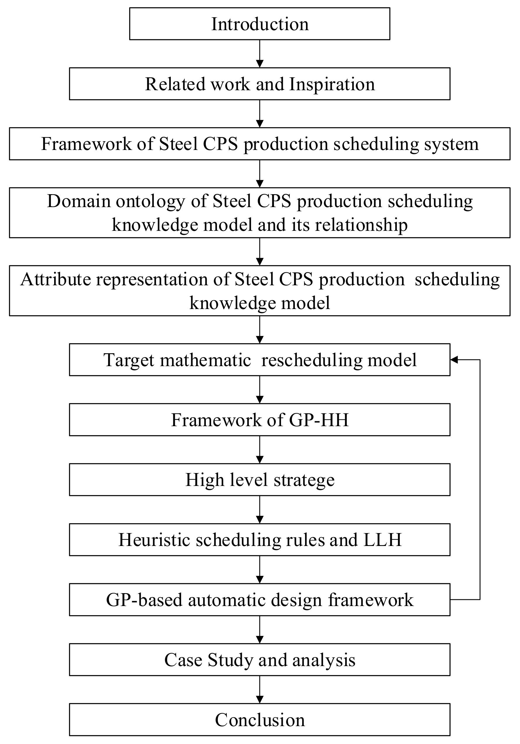
With the rapid development of information technology, the cyber-physical system (cyber-physical system, CPS) concept has been widely used, which provides a new solution for steel production scheduling. CPS is an intelligent system integrating computing, communication, and control to realize deep integration and interactive feedback between the physical world and the information world. The combination of CPS and steel production scheduling systems makes up for the difficulty of dynamic scheduling of steel production in a complex environment and provides the possibility of developing steel production to intelligent manufacturing. Therefore, a scheduling model for steel CPS orientation was proposed. For steel CPS’s complex dynamic scheduling scenario, modeling alone is not enough to solve the problem. Therefore, a universal genetic programming-based hyper-heuristic algorithm (genetic programming-based hyper-heuristic, GP-HH) was proposed. Finally, the performance of the algorithm is verified by rescheduling cases based on equipment disturbance. The whole work conducted in the paper is shown in Figure 1.

The rest of this paper is organized as follows. Section 2 is related work about CPS, steel scheduling, and hyper-heuristic algorithms. Section 3 established the construction of a steel CPS production scheduling model based on ontology. Section 4 describes the design of a hyper-heuristic algorithm based on genetic programming. Section 5 shows the simulation results of GP-HH, and Section 6 provides the conclusions and future works.

2. Related Work

2.1. CPS

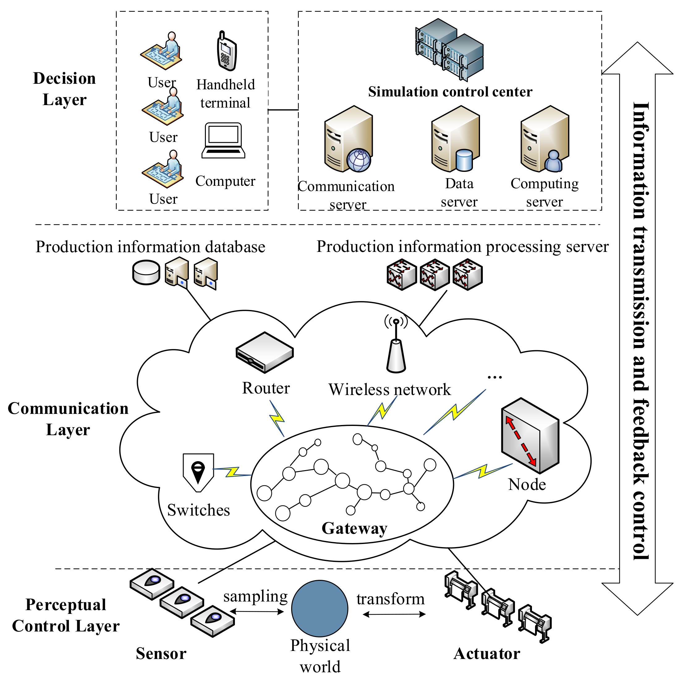
In recent years, CPS has been widely used in aerospace, rail transit, power grid, water resource scheduling, industrial advanced manufacturing and automation, emerging smart home, smart agriculture, and other fields [4,5,6]. CPS is widely regarded as a standard technology closely combining industrial automation and information technology. It is a controllable, credible, and scalable networked physical equipment and software integrated interactive system based on environmental perception and deeply integrating computing, communication, and control [7]. It can be applied in the embedded field or composed of superimposed systems or components through an integrated application, communication, the cloud platform, and big data from the CPS architecture [8]. It can be seen that CPS is a multi-dimensional complex system of an integrated computing system, network system, and physical system. Its core is the deep integration and close cooperation of high-performance computing, real-time communication, and accurately controllable capabilities, which also meets the needs of efficient, reliable, and accurate management and collaboration of physical entities. Through literature review, analysis, induction, and integration of similar studies [9,10], the paper summarizes the classical architecture of CPS, mainly including the perceptual control layer, communication layer, and decision layer (as shown in Figure 2).

The perceptual control layer is the interface between the CPS’s information system and the physical system. It senses the state and events of physical devices in the system by the sensor, realizes the information perception of physical entities, and then executes control instructions through actuators to change the state of physical entities [11].

The communication layer is the channel for information and command transmission in the CPS, including various gateways, nodes, wireless networks. Through the information communication between nodes and gateways, the interaction and cooperation of CPS modules and subsystems are realized [12].

The decision layer includes the computing system, communication system, data system, and simulation control center. The virtual entity of the simulation control center stores the digital geometric model, behavior state model, and information model of physical entities and then realizes the interconnection, control, and decision-making between physical entities through the theoretical data [13].

A summary of the published works is provided in Appendix A with a detailed review. Form Appendix A, different from the traditional information system modeling method, CPS contains massive information physical interaction examples involving the flow of energy and information. According to the specific application, the modeling methods are also different. How to truly reflect the operation mode of a real system is the key to modeling. Considering the complexity of the steel production scheduling system (physical system), CPS is a dynamic system to realize mutual connection and coordination of iron and steel production. There are many studies on steel production scheduling, but there are few reports on the combination of steel production scheduling and CPS.

2.2. Knowledge-Based of Steel Production Scheduling

The traditional research on steel production scheduling problems focuses on steel production scheduling modeling and algorithm design. Theoretically, on the one hand, the model can be built very complex and meet certain conditions or assumptions [14]. On the other hand, the algorithm design can obtain sufficient convergence speed and accuracy, and the solution set of scheduling problems can also be obtained. However, for different problems, the model is relatively single, and the scene adaptability is not strong. In the implementation, for this complex scheduling problem, even if the model is optimized in theory, it is still difficult to be effectively applied to optimize the steel production schedule because of the lack of corresponding technical means. With the rapid development of knowledge engineering, cloud computing, big data, digital twin, and CPS, it is possible to study the production schedule based on knowledge engineering and realize the informatization, integration, knowledge, and intelligence of steel production scheduling system.

The knowledgeable manufacturing system is an in-depth, intelligent manufacturing system with the main characteristics of self-adaptation, self-learning, self-evolution, self-reconstruction, self-training, and self-maintenance, emphasizing the mining, processing, and utilization of the production knowledge contained in the manufacturing system [15,16,17]. Knowledge-based production scheduling has gradually become the focus of research. Jiang GZ et al. studied the steel production scheduling knowledge network system and established the steel mixed process knowledge base system and knowledgeable encapsulation method [18,19]. Xu BZ et al. formally described the energy consumption elements in the knowledge network by using the knowledge network theory and multi granularity modular ontology technology and proposed the knowledge network energy consumption model of discrete manufacturing systems [20]. However, there are still barriers to knowledge acquisition in knowledge-based scheduling, which brings great difficulties to knowledge-based production scheduling.

A summary of the published works is provided in Appendix B with a detailed review. From Appendix B, most of the existing steel production scheduling involves scheduling for specific problems, and the models and algorithms are not universal and reusable. Without establishing steel production scheduling based on the combination of knowledge engineering and CPS, it is impossible to effectively identify and manage the similarities and differences between the scheduling model knowledge. The massive production data of CPS contains rich scheduling knowledge. After mining, valuable laws can be obtained, which is helpful to knowledge management and decision optimization in the field of production scheduling. In this way, the production scheduling knowledge representation of the steel CPS-oriented model based on ontology is significant.

2.3. Hyper-Heuristic Algorithm

The hyper-heuristic algorithm is a new optimization method. It is an automatic method for selecting or generating heuristics to solve computational search problems. It can solve cross problem areas [21]. It is widely used in vehicle routing [22], nurse scheduling [23], reinforcement learning [24], production scheduling [25,26] and has great application potential.

In complex production scheduling, a single heuristic algorithm or heuristic rule is challenging to consider accurately and quickly solve the dynamic scheduling problem of steel production. It is necessary to design an algorithm with strong universality and quickly solve the production scheduling problem in different scenarios. Hyper-heuristic has a good performance in this field [27]. It manages a series of low-level heuristics (low-level heuristics, LLH) through different high-level strategies to select and generate new heuristic operators to search the solution space. Facing various steel production scheduling problems, the hyper-heuristic can find appropriate combination rules through efficient search strategy and quickly solve the dynamic scheduling problems in different scenarios. A summary of the published works is provided in Appendix C with a detailed review.

2.4. Inspiration

From the literature, the research on steel production scheduling mainly focuses on modeling and scheduling algorithm design, as shown in

Table 1. The research gap of related work.

Reference Number/Publication Year	CPS Modeling and Verification	Scheduling Algorithm	Knowledge Scheduling	Hyper-Heuristic	Knowledge-Based Steel CPS Production Scheduling and Algorithm
[6]/2019	✓
[7]/2019	✓
[8]/2018	✓
[9]/2019	✓
[10]/2018	✓
[14]/2021		✓
[15]/2016			✓
[16]/2016		✓	✓
[18]/2018			✓
[19]/2020			✓
[20]/2017			✓
[21]/2019				✓
[22]/2020		✓		✓
[23]/2016		✓		✓
[24]/2018				✓
[25]/2015		✓		✓
[26]/2020		✓		✓

. There is less research on the production scheduling theory and application of steel CPS based on knowledge engineering, especially the research on knowledge modeling of steel CPS production scheduling model.

The steel industry is a typical process industry. As the main body of the whole process, blast charge, converter, refining charge, ladle, continuous casting billet, hot rolled piece, and cold rolled piece are “black boxes,” that is, the outside cannot obtain the internal information of each reactor. Even if the big data control platform is established, it can still not accurately grasp the physical and chemical changes in the “black box.” The digital sensing technology based on CPS can describe the “black box” changes and make intelligent decisions and control. Therefore, a scheduling model for steel CPS orientation was proposed the first time. In the steel CPS, the steel industry will use the information technologies such as the Internet of things, big data, and cloud computing to establish an integrated management and control platform. For the complex dynamic scheduling scenario of steel CPS, modeling alone is not enough to solve the problem. Therefore, a universal GP-HH algorithm was proposed to solve the production scheduling model under multiple disturbances. In this way, the steel industry will overcome the isolated and single process solution in the past and achieve “in-depth perception of information, network interconnection, accurate, coordinated control, and optimized intelligent decision-making.”

3. Ontology-Based Steel CPS-Oriented Production Scheduling Knowledge Model

3.1. Framework of Steel CPS-Oriented Production Scheduling System

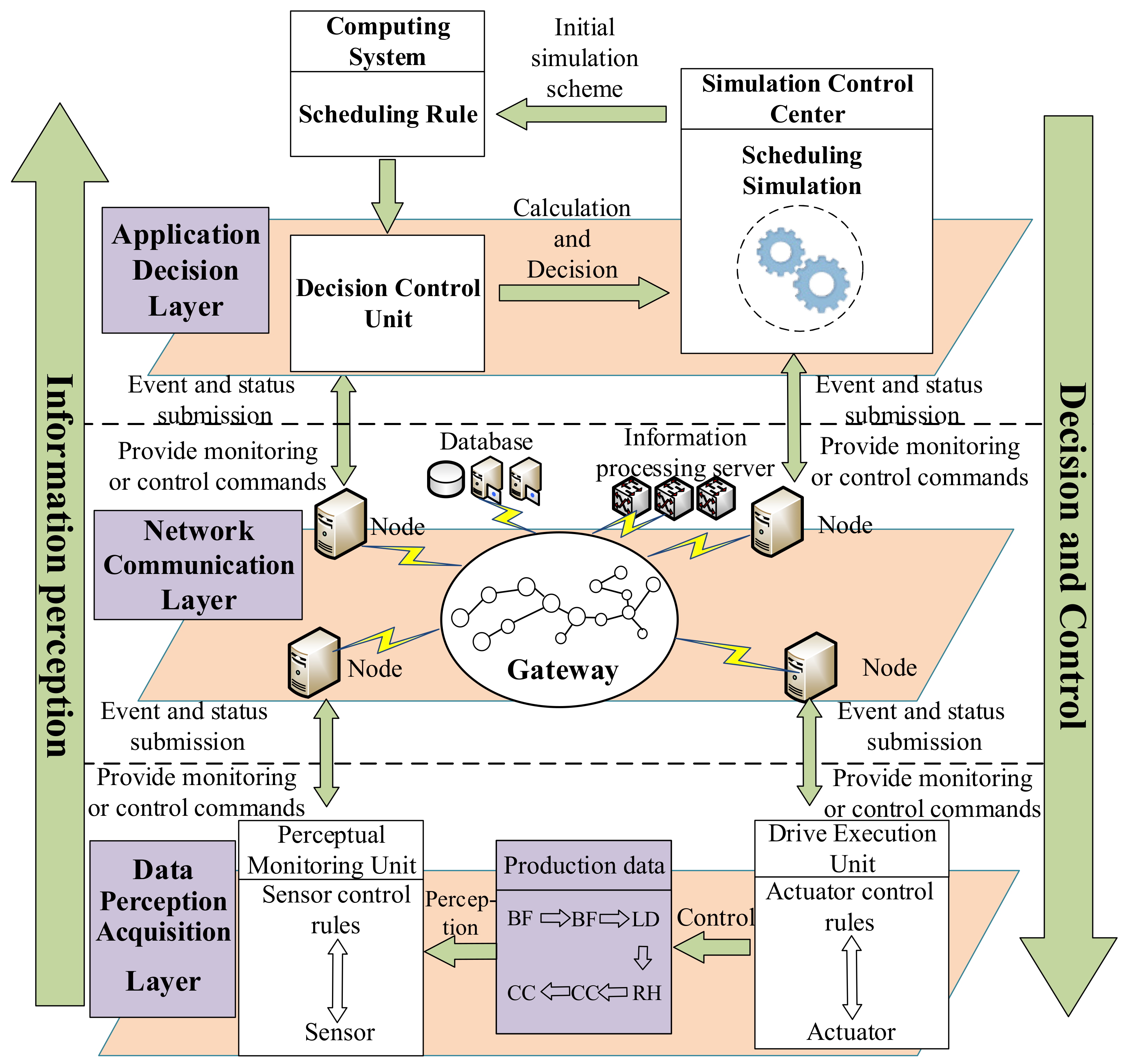
In addition to the typical characteristics of the traditional steel production scheduling system, the steel CPS-oriented production scheduling system also has the features of CPS. Under the unique perception environment of CPS, it should consider the production scheduling problem of the steel production scheduling system (physical system) and perceive the dynamic disturbance events in steel production scheduling. The mapping of scheduling events in steel production scheduling system (information system) to study the production scheduling problem of steel CPS under the combination of information world and physical world. As shown in Figure 3, it is the architecture of steel production scheduling system for CPS-oriented, divided into application decision layer, network communication layer, and data perception acquisition layer.

(1) Data Perception Acquisition Layer

This layer is the interface between the physical system and the information system in CPS. It mainly realizes the information perception and accurate control in the steel production scheduling. Information perception has the characteristics of ubiquitous sensing, fine-grained sensing content, wide sensing area. The ubiquity of sensing means that its sensing terminals distribute many sensing monitoring units, including sensors, wireless handheld terminals, RFID (radio frequency identification), processors for information integration, and data storage. It can sense the equipment status and process of the steel production process through sensors and control rules. Perceived content granularity refers to the fine-grained definition of each process information content. The wide sensing area means that its sensing terminals are distributed in all links of steel production and include the process control information feedback by the control execution unit in the computing system to optimize the main parameters of each process and accurately control the production.

(2) Network Communication Layer

This layer realizes the efficient transmission, storage, and processing of information in the steel production scheduling. It includes various base stations, wireless networks, wired networks, handheld terminals, bridges, and RFID antennas. The embedded computer, embedded software, and the feedback loop of nodes and networks are formed to monitor and control equipment status in the physical system and allocate production tasks. At the same time, the production status and process status of the underlying equipment are feedback to the database and information processing server. The information processing server will perform data cleaning, classification, filtering, fusion, secondary processing, and other operations on heterogeneous information, convert it into a unified data mode, and transmit it to the application decision-making layer through industrial ethernet and wireless sensor network.

(3) Application Decision Layer

This layer includes a computing system, decision control unit, and simulation control center, which mainly realizes the intelligent decision-making of steel production scheduling and the scheme optimization. The computing system is the brain of the steel CPS production system. The data sensing acquisition layer can obtain the workshop’s bottom equipment, personnel, and production progress in real-time, respond to the scheduling request, calculate, and make intelligent decisions. The simulation control center is the model repository of the steel CPS production system, responsible for storing real-time scheduling data and generating an initial scheduling scheme. The decision control unit integrates and optimizes the initial scheduling scheme by calculating the predefined scheduling rules in the system to realize the information perception and control decision of steel production scheduling.

3.2. Definition of Domain Ontology of Steel CPS Production Scheduling Knowledge Model

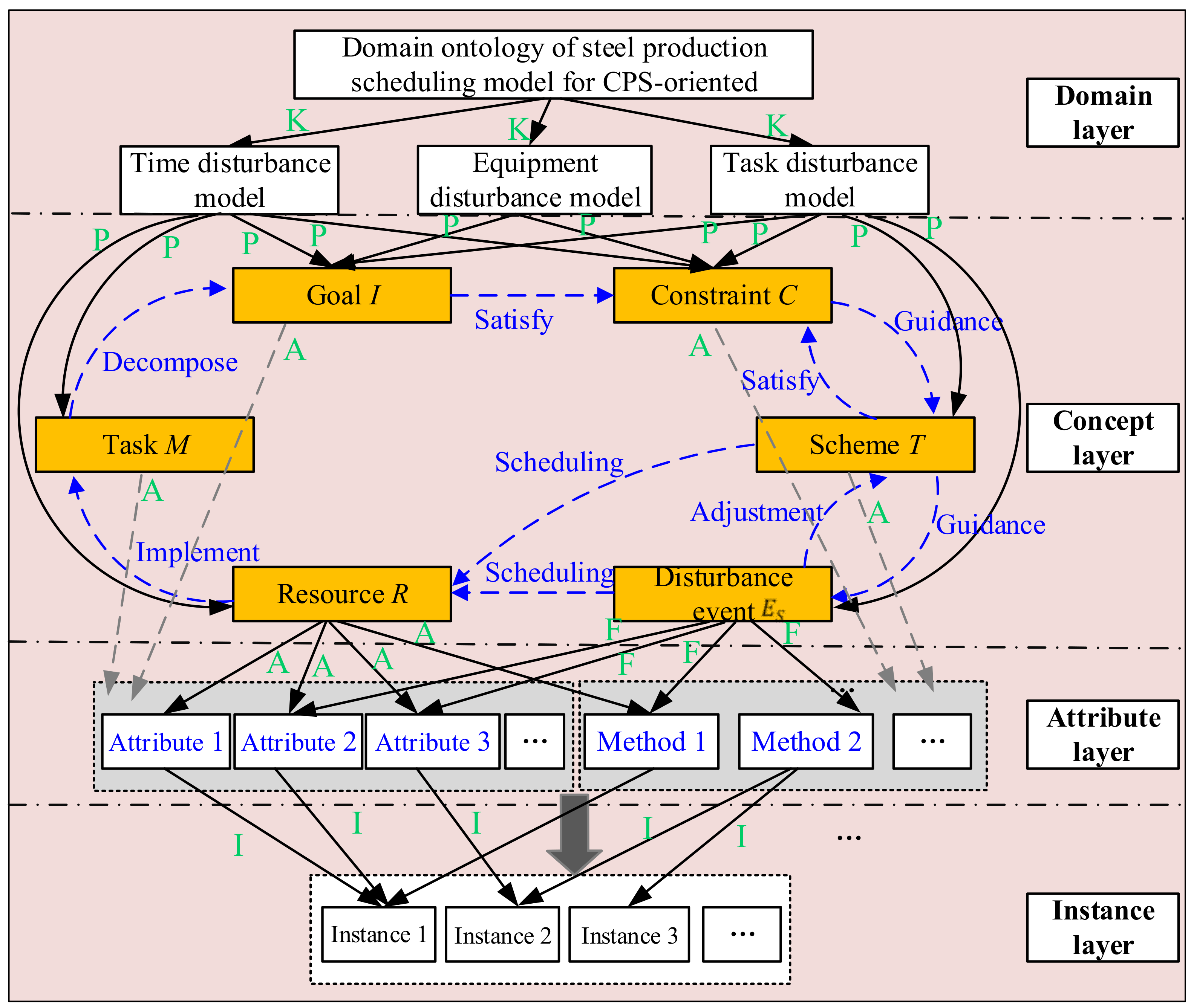
The construction of the steel CPS production scheduling ontology model is reflected in the extraction of ontology concepts in related fields and the inheritance of relationships. The extracted concepts should contain enough as much information as possible and simplify the ontology [28,29,30]. According to the modeling method proposed in references [31,32], combined with the essence and concept description of steel production scheduling process in CPS environment, the core ontology concepts are abstracted, which mainly include six categories: Task M, Goal I, Constraint C, disturbance event $E_S$, resource R and scheduling scheme T. The attributes between conceptual ontologies include decomposition, satisfaction, guidance, adjustment, scheduling, and execution. Other relationships include kind of (K means inheritance), part of (P means partial), attribute of (A means attribute), function of (F means function), and instance of (I means instance).

The domain ontology of the SPSCPS (steel production scheduling of CPS, SPSCPS) problem can be defined with a five-tuple, as shown in Equation (1).

$$SPSCPS\_Ontology=\left\{C,A,R,H, Y\right\}$$

(1)

In the equation, C is the concept set, A is the attribute set, R is the relationship set, H is the dependency set of the concept, and Y is the axiom set.

The above-selected concepts and defined attributes can describe the domain ontology of the steel production scheduling model in the CPS environment. As shown in Figure 4, it is a four-level domain ontology model of steel CPS production scheduling, including domain layer, concept layer, attribute layer, and instance layer. The domain layer represents the top-level concepts in the field. The concepts with inheritance and partial relationship are represented on the concept layer. The concepts, related attribute information, and methods play the role of description at the attribute layer. The instance generated by the combination of method and attribute is in the instance layer. The relationship between these concepts is that the task guides the steel production scheduling problem. Task (R) is decomposed into multiple subtasks and activities characterized by goal (I). When constraint (C) is satisfied, a guidance scheme (T) is generated to realize multi-objective optimization. Then according to the disturbance event ($E_S$) adjust the scheduling scheme(T) and optimize the resource (R) allocation to make the production go smoothly.

3.3. Attribute Representation of Steel CPS Production Scheduling Knowledge Model

The ontology relation graph can directly represent the scheduling ontology model, but to study the properties of scheduling domain knowledge ontology is necessary. It can define various core concepts, basic attributes, and attribute relationships. The domain ontology of the steel CPS scheduling problem can be conceptualized as Equation (2).

$$SPSCPS\_ConceptOntology=\left\{MConceptSet,RConceptSet\right\}$$

(2)

$MConceptSet$ is the set of conceptual ontologies in steel CPS scheduling, including multiple conceptual ontologies. $RConceptSet$ is the set of relationships between concept ontologies. The concept ontology set can be further refined into Equation (3).

$$MConceptSet=\left\{NConcept,PConcept\right\}$$

(3)

$NConcept$ is the name of the concept ontology. $PConcept$ is the attribute of the concept ontology. According to the above, the conceptual ontology of the scheduling task(M) can be described as Equation (4).

$$M=\left\{M_{Info},M_{Attribute},M_{RelSet},su{b}_{M1},su{b}_{M2},\dots ,su{b}_{MN}\right\}$$

(4)

In the equation, $M$ is the task. $M_{Info}$ is the task information. $M_{Attribute}$ is task properties. $M_{RelSet}$ represents the time sequence, constraint, or decomposition relationship between subtasks. $su{b}_{MN}$ is the subtask.

Scheduling goal(I) is an evaluation measure of indicators, including time indicators, production cost indicators, quality indicators, equipment OEE. The goal ontology and its attribute concept can be defined as Equation (5).

$$I=\left\{I_{Set},I_{Attribute},I_{RelSet}\right\}$$

(5)

$I_{Set}$ is the set of each indicator type. $I_{Attribute}$ is indicator attributes, including weight coefficient, inclusion, conflict, and other attributes. $I_{RelSet}$ is the relationship between multiple objectives.

Scheduling constraint(C) is the condition to ensure smooth production and on-time delivery. Its attribute concept can be defined as Equation (6).

$$C=\left\{C_{Set},C_{Attribute},C_{RelSet}\right\}$$

(6)

$C_{Set}$ is a set of constraint types, including process constraints, time constraints, sequence constraints. $C_{Attribute}$ is the attribute of constraints. $C_{RelSet}$ is the relationship between constraints, such as inclusion, combination, mutual exclusion.

The disturbance is an unpredictable event that affects the scheduling scheme. The disturbance event is regarded as a domain ontology in steel CPS production scheduling, and its conceptual ontology can be defined as Equation (7).

$$E_S=\left\{E_S{}_{Info},E_S{}_{Attribute},E_S{}_{RelSet}\right\}$$

(7)

$E_S{}_{Info}$ is the description information of $E_S, E_S{}_{Attribute}$ is the attribute of $E_S, E_S{}_{RelSet}$ is the attribute relationship of $E_S$.

Scheduling resource guarantees time and cost index in steel production scheduling, and its attribute concept ontology is Equation (8).

$$R=\left\{R_{Info},R_{Attribute},R_{RelSet}\right\}$$

(8)

$R_{Info}$ is the description information of R, $R_{Attribute}$ is the attribute of R,$R_{RelSet}$ is the relationship between resources, including attribute relationship, attribute relationship, hierarchical relationship, instance relationship.

The scheduling scheme (T) is a solution to allocate resources under meeting constraints and indicators to optimize objectives, including the re-optimization of disturbance events, which has a specific mapping relationship with other domains ontologies. It can be formalized as Equation (9).

$$T=f_i\left(M,I,C,E_S,R\right)=\{\begin{array}{c}{M}_{Info},M_{Attribute},M_{RelSet},su{b}_{M1},su{b}_{M2},\dots ,su{b}_{MN}\\ I_{Set},I_{Attribute},I_{RelSet}\\ C_{Set},C_{Attribute},C_{RelSet}\\ E_S{}_{Info},E_S{}_{Attribute},E_S{}_{RelSet}\\ R_{Info},R_{Attribute},R_{RelSet}\end{array}{\}}^T$$

(9)

4. Hyper-Heuristic Algorithm Based on Genetic Programming for Steel CPS

4.1. Target Mathematical Model

There are taking the equipment disturbance of steel production as an example. In the steelmaking and continuous casting (steelmaking and continuous casting, SCC) scheduling problem based on equipment disturbance, the processing equipment and a start time of each charge after disturbance is variables to be solved, all operating equipment and time form an optional value range, and the process requirements to be followed in the converter, refining, and continuous casting process form a set of constraints. The following assumptions are made for the equipment disturbance problem: (1) The initial scheduling scheme has been implemented before the equipment fails. (2) The interrupted charge can continue processing on other parallel equipment. (3) Adjust the casting speed of the continuous caster or the operation time of the converter and refining to repair the conflict between time and resources. (4) The repair time of faulty equipment is known. (5) Equipment disturbance occurs only in the converter or refining stage. The SCC scheduling model based on the disturbance of converter or refining equipment is as follows.

$$\min f={\displaystyle \sum }_{i\in N}{\displaystyle \sum }_{j\in M}({\omega }_1\times A_{ij}+{\omega }_2\times B_{ij})$$

(10)

$$A_{ij}=\left|T_{ij}-T_{ij}^{\prime }\right|/\max \left\{\left|T_{ij},T_{ij}^{\prime }\right|\right\}$$

(11)

$$B_{ij}=\min \left\{\max \left\{\left|m_{ij}-m_{ij}^{\prime }\right|,0\right\},1\right\}$$

(12)

Equation (10) is the objective function, representing the degree of the difference caused by minimizing equipment failure after equipment disturbance. Equations (11) and (12) are differential coefficient equations. i = {1, 2,…, N}, is the charge number. j = {1,2,3}, corresponding to steelmaking, refining, and continuous casting stages.$A_{ij}$ and $B_{ij}$ is the indicates difference of start-up time and equipment assignment. ${\omega }_1,{\omega }_2$ is the coefficient of $A_{ij}$ and $B_{ij}$.$m_{ij} \mathrm{and} m_{ij}^{\prime }$ is the processing equipment of charge before and after rescheduling.$T_{ij}$ and $T_{ij}^{\prime }$ is the start-up time of charge before and after rescheduling.

$$s.t. T_{i,j+1}^{\prime }\ge T_{ij}^{\prime }+T{S}_{ij}^{\prime }$$

(13)

Equation (13) represents the conflict constraint that each charge operation cannot be processed in multiple stages simultaneously.$T{S}_{ij}^{\prime }$ is the processing time of charge after rescheduling.

$${{\displaystyle \sum }}_{h=1}^{M_j}{S}_{ijh}=1$$

(14)

$$T{O}_{ij}^{\prime }=T_{ij}^{\prime }+T{S}_{ij}^{\prime }$$

(15)

Equations (14) and (15) represent charge $L_{ij}$ can only be processed by a piece of equipment at a stage and is not interrupted.$S_{ijh}$ is the processing status. $M_j$ is the set of parallel machines in stage j.$T{O}_{ij}^{\prime }$ is the end-up time of charge after rescheduling.

$$T_{i+1,j}^{\prime }=T{O}_{ij}^{\prime }, J=3$$

(16)

$$T_{i,j+1}^{\prime }-T{O}_{ij}^{\prime }\le T{P}_{ij}^{\prime }$$

(17)

Equation (16) represents the continuous casting constraint of the adjacent charge. Equation (17) indicates an upper limit constraint on the transportation time of the charge between each process.$T{P}_{ij}^{\prime }$ is the maximum transportation time of charge from stage j to j + 1.

$$\left(T{O}_{ij}^{\prime }-T_{ij}^{\prime }\right) - \left(T{O}_{ij}-T_{ij}\right) \le T{Z}_{ij}^{\prime }, J=3$$

(18)

$$I_{q_1}\cap I_{q_2}=\varnothing$$

(19)

$$\left(m_{ijh}^{\prime }\ne m_{ijh}^b\right)\vee \left(T_{ij}^{\prime }\ge T_b\right)$$

(20)

Equation (18) indicates that the casting time before and after charge rescheduling cannot exceed the caster’s upper limit of casting speed adjustment. Equation (19) indicates that one charge can only be processed in one casting. Equation (20) indicates that the charge interrupted by equipment failure is transferred to other parallel equipment for processing.$T{O}_{ij }\mathrm{and} T{O}_{ij}^{\prime }$ is the end-up time of charge before and after rescheduling.$I_q$ is the set of charge of the q-th casting.$m_{ijh}^b$ indicates charge i is processing at the failed equipment $m_{ij}$ in stage j. $T_b$ is the fault start time.

4.2. Hyper-Heuristic Algorithm Framework Based on Genetic Programming

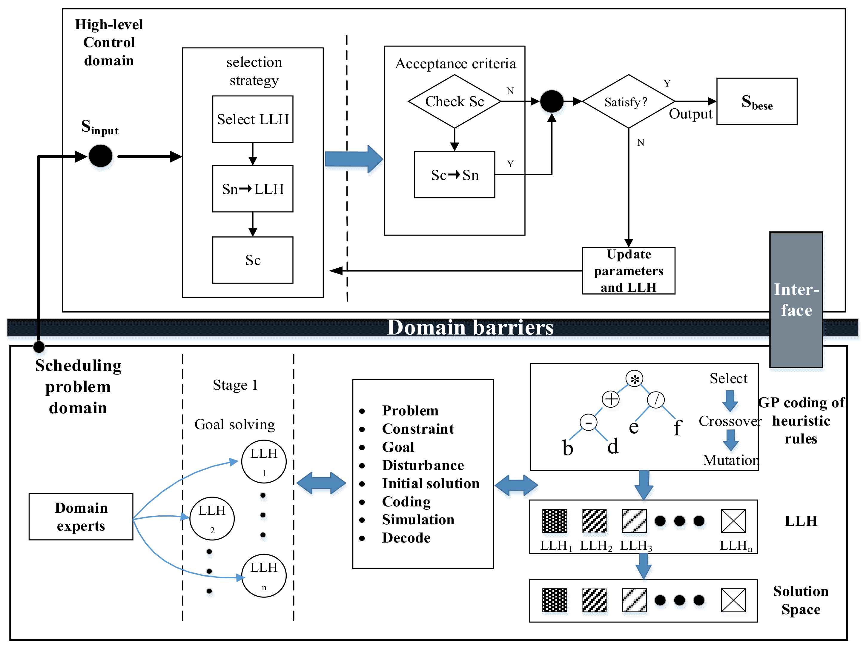
In this paper, genetic programming (genetic programming, GP) based hyper-heuristic (GP-based hyper-heuristic, GP-HH) is proposed to solve the disturbance-based steel production scheduling problem. Simple rules generally consider a single factor of the furnace, equipment, or transportation tool and do not consider disturbance. Therefore, the problem model proposed in this paper is more complex. The furnace, equipment, and disturbance at each time have multiple different attributes, so to make full use of multi-factor information of furnace, equipment, and disturbances make the rules containing this information produce excellent scheduling rules. GP-HH uses GP to generate some excellent heuristic rules to form a heuristic scheduling rule set. The process of GP generating rules can be calculated offline. Using the GP-HH, you only need to search and select the heuristic rule set. On the one hand, it can make the convergence speed faster and reduce the operation time of the algorithm; on the other hand, the global search ability of the algorithm becomes more robust, which makes up for the deficiency that the rule-based heuristic can only obtain the suboptimal solution. Figure 5 shows the hyper-heuristic algorithm framework of genetic programming, divided into two parts: the upper control and lower problem domains.

The high-level strategy is designed to select the low-level heuristic (low-level heuristic, LLH) in the upper control domain. The LLH is represented and generated by GP. The information is transmitted through the preset interface in the domain barrier so that the high-level strategy and the LLH are independent of each other. On the one hand, the high-level strategy transfers scheduling strategy and other information through the low-level operator and indirectly calls the LLH for the solution; on the other hand, in the process of solving, the LLH returns the quality of the solution and the operator execution time to the high-level strategy to guide the generation of operator scheduling strategy.

4.3. High-Level Strategy

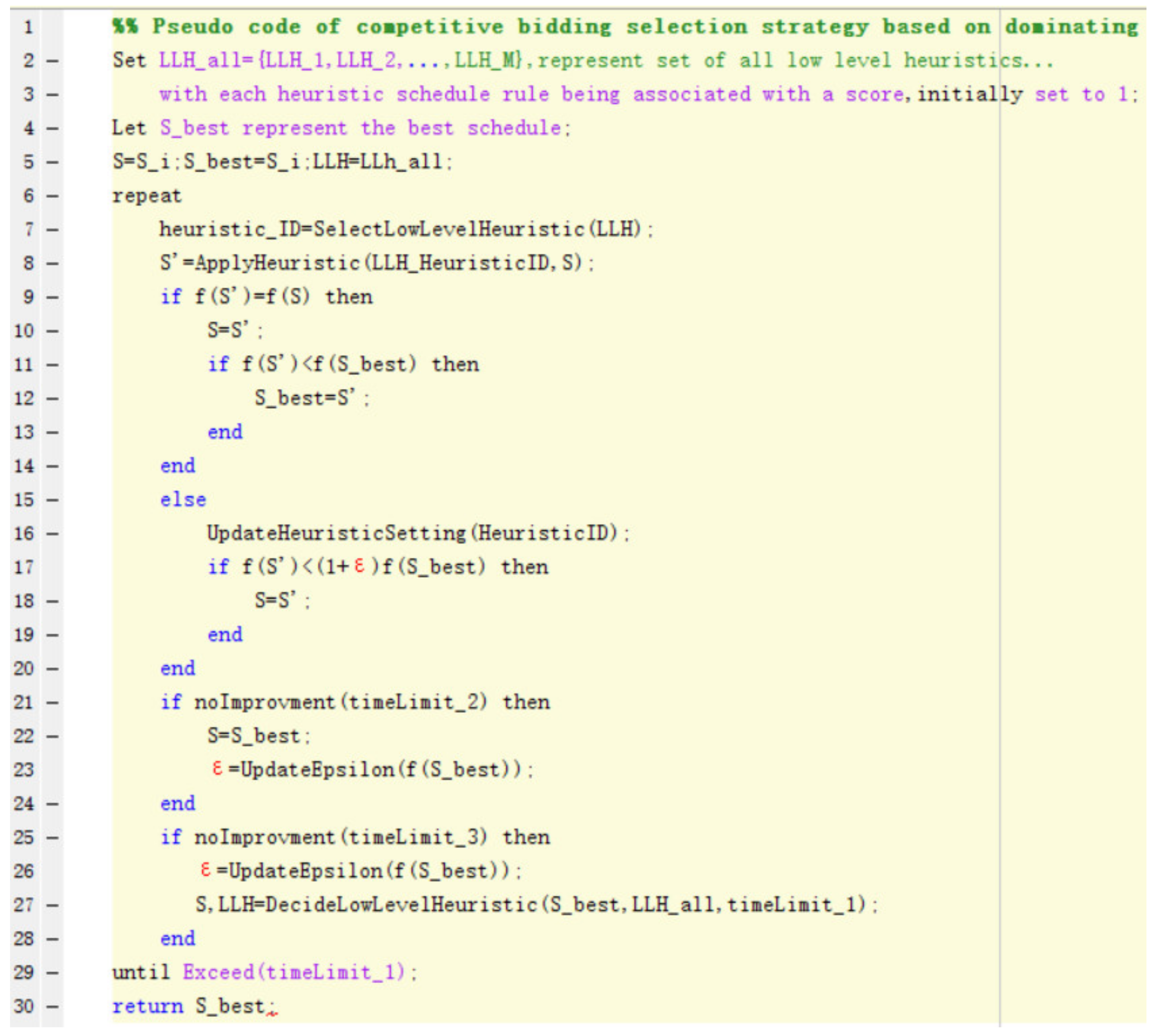
The high-level strategy of the hyper-heuristic algorithm manages the LLH operators. Selecting an appropriate high-level strategy is very important to solve the scheduling model. This paper adopts the learning-based high-level selection strategy, and the pseudo-code is shown in Figure 6. The heuristics selected in Lines 8–25 and 27–28 are applied to solve the rescheduling model. At first, each heuristic gets a score of 1, making the probability of each heuristic being selected equally. The first hyper-heuristic always maintains the best solution, expressed as ${\mathrm{S}}_{best}$ (Lines 10–12) and keep track of each improved solution. The move acceptance component (Lines 10–21) is a critical value controlled by parameters $\mathsf{\epsilon }$. All improved changes are acceptable only when the performance of a solution is better than that of the optimal solution (Line 18) $\left(1+\mathsf{\epsilon }\right)$ the performance, the scheme will be accepted. When the optimal solution is no longer optimized in a limited time,$\mathsf{\epsilon }$ will be improved (Line 24).

$$f\left(x\right) = \left(\left[log\left(x\right)\right] + rand\left(1,\left[log\left(x\right)\right]\right)\right)/x$$

(21)

$X=f\left({\mathrm{S}}_{best}\right)$ is the target value of the optimal solution, its threshold is [lb, ub], and returns a random integer [lb, ub]. If $f\left({\mathrm{S}}_{best}\right)$ is 0, the algorithm terminates. This case is not considered to be updated in the threshold.

When the second hyper-heuristic starts operation (Lines 26–29), the quality of time-limited Solution 2 is not improved (Lines 26). It means the heuristic algorithm pool (LLH) from the underlying heuristic to all solution sets (expressed as $LL{H}_{all}$) will be used in the next stage, the idea of dominance-based heuristic selection will be introduced, and the score of each underlying heuristic will be dynamically adjusted. First, $\mathsf{\epsilon }$ in the first hyper-heuristic algorithm is updated in the same way and remains unchanged. Then, according to a certain number, a greedy strategy is used to drive all bottom heuristic operators to fix the number. Next, this hyper-heuristic constructs solutions corresponding to each production bottom heuristic operator, reflecting the relationship between the goal realization and the number of bottom heuristics in each step. At the end of this phase, the non-dominated solution is used from the whole solution set to obtain a Pareto frontier. If more than one low-level heuristic finally produces the same target value at the Pareto front, they will all be selected into the algorithm pool. The number of occurrences of each underlying heuristic is assigned as its score and used for the first hyper-heuristic.

At each step, at a fixed time $\mathsf{\tau }$, each underlying heuristic is cycled as the same input when considering the threshold change acceptance method (threshold move acceptance method). Some LLH may take more time than others. Therefore, we use the circular method to treat all LLH equally. In each $LL{H}_{small}$, $LL{H}_{medium}$, $LLH{ }_{large}$ heuristic, $\mathsf{\tau }$ is assigned 5 n/q, n/q respectively and performs one iteration, n represents the number of activities, and q represents the number of projects. If the LLH generates the same solution as the input, the call is ignored. Otherwise, the new solution and the target are recorded, and the LLH generates the solution scheme. If all heuristics cannot produce new solutions, they will be reconsidered together. Once all heuristics are used as input and processed at this stage, the optimal solution scheme will be propagated as the input of the following greedy strategy. If the total given limit time (Time-Limit1) times out, all steps are completed with the relevant solution set before the termination of the second layer hyper-heuristic.

4.4. Heuristic Scheduling Rules and LLH

Taking SCC as an example, there are four common disturbances: time disturbance, equipment disturbance, process disturbance, and task disturbance. For these disturbance events, different rules are used to adjust the production scheduling plan.

(1) Minimum of conflict time R1

Set $X_{ijk},Y_{ijk}$ is the start time and finish time of $m_{ijk}, X_{ijk}^{\prime }, Y_{ijk}^{\prime }$ is the start time and finish time of $m_{ijk}^{\prime }$.$m_{ijk}$ is the k-th process of the j-th charge in the i-th casting in equipment m, m is the equipment number, m = 1, 2,…, $M^{*}$.$T_m^{m_1}$ is the waiting time from m to $m_1. P_{ijk}$ is the processing time.

$$X_{ijk}=X_{ij,k+1}-T_m^{m_1}-P_{ijk}$$

(22)

The $\mathsf{\Delta }\mathrm{T}$ is the conflict time between $m_{ijk}$ and $m_{ijk}^{\prime }$.

$$\mathsf{\Delta }\mathrm{T}=\min \left\{Y_{ijk}^{\prime },Y_{ijk}\right\}-\max \left\{X_{ijk}^{\prime },X_{ijk}\right\}$$

(23)

When $\mathsf{\Delta }\mathrm{T}\le 0, m_{ijk}$ and $m_{ijk}^{\prime }$ have no time conflicts on the equipment m, operation $m_{ij,k+1}$ waiting time $w_{ijk}$ on equipment is 0. When $\mathsf{\Delta }\mathrm{T}>0$, operation $m_{ij,k+1}$ have job time conflict on the equipment m, operation $m_{ij,k+1}$ waiting time $w_{ij,k+1}$ as Equation (24)

$$w_{ij,k+1}=X_{ij,k+1}-T_m^{m_1}-X_{ijk}^{\prime }$$

(24)

Because $X_{ij,k+1}=X_{ijk}+T_m^{m_1}+P_{ijk}$, so

$$\begin{array}{ll}{w}_{ij,k+1}& =X_{ijk}+T_m^{m_1}+P_{ijk}-T_m^{m_1}-X_{ijk}^{\prime }\\ & =X_{ijk}+P_{ijk}-X_{ijk}^{\prime }=\mathsf{\Delta }\mathrm{T}\end{array}$$

(25)

When $m_{ijk}$ and $m_{ijk}^{\prime }$ have a time conflict on the equipment m, operation $m_{ij,k+1}$ watting time is $w_{ij,k+1}$, it is conflict value $\mathsf{\Delta }\mathrm{T}$. Therefore, in the process of equipment assignment, selecting the equipment that minimizes the conflict value of operation time between operations from multiple optional pieces of equipment that can process charge operation as the processing equipment can ensure that the waiting time for an operation on the equipment is minimized as far as possible. Thus, the waiting time of operation and processing between adjacent equipment in the same charge is minimized as far as possible.

$$m_{ijk}=1, \mathrm{m}=\arg \min \left\{\mathsf{\Delta }{\mathrm{T}}_{m_1}\right|m_1\in M_{m_{ijk}}^{*}\}$$

(26)

(2) Shortest transportation time R2

$$X_{ij,k+1}=X_{ijk}+T_m^{m_1}+P_{ijk}$$

(27)

When $T_m^{m_1}$ is shorter, the operation $m_{ijk}$ is bigger for the start time. There is a slight possibility of job conflict between other operations and $m_{ijk}$. When the operation time conflict value between operations is smaller, the waiting time generated by the charge on the equipment will be minimized to minimize the operation and processing waiting time between adjacent equipment. The assignment method based on the rule of shortest transportation time between equipment is from $M_{m_{ijk}}^{*}$ among the optional equipment. The processing equipment with the shortest transportation time between it and its subsequent process equipment is selected as the operating equipment.

$$m_{ijk}=1, \mathrm{m}=\arg \min \left\{T_{m_1,m_2}\right|m_1\in M_{m_{ijk}}^{*}\}$$

(28)

(3) Minimum total equipment conflict time R3

Assume $P_m$ is the set of operations on equipment m,$P_m=\left\{p_m^1,p_m^2,\dots ,p_m^l,\dots ,p_m^{b_m}\right\}$, $p_m^l$ is the l-th operation on equipment m.$b_m$ is the total number of operations on the device. $\mathsf{\Delta }{\mathrm{T}}_m$ is the sum of operation time conflict values of all the charges on equipment m.

$$\mathsf{\Delta }{\mathrm{T}}_m={\displaystyle \sum }_{l_1}^{b_m-1}{\displaystyle \sum }_{l_2=l_1+1}^{b_m}\max \left\{0,\min \left(x_{p_m^{l_1}}+P_{p_m^{l_1}},x_{p_m^{l_2}}+P_{p_m^{l_2}}\right)-\max \left(x_{p_m^{l_1}},x_{p_m^{l_2}}\right)\right\}$$

(29)

The minimum rule of total conflict time of equipment refers to the operation $m_{ijk}$ assigns equipment, it starts from the $M_{m_{ijk}}^{*}$ capable of machining operation to select the equipment with the shortest total conflict time as the operation $m_{ijk}$ processing equipment.

$$m_{ijk}=1, \mathrm{m}=\arg \min \left\{Q_{m_1}\right|m_1\in M_{m_{ijk}}^{*}\}$$

(30)

(4) Random selection R4

The random selection rule refers to the operation $m_{ijk}$ assigns a piece of equipment, it randomly selects equipment from multiple machines as $m_{ijk}$’s processing equipment.

$$m_{ijk}=1, \mathrm{m}=\mathrm{random}\left\{m_1\right|m_1\in M_{m_{ijk}}^{*}\}$$

(31)

According to the rules, the following heuristic scheduling rules based on rule priority are established.

(1) $S_{R1}$: Minimum of conflict time R1, shortest transportation time R2, random selection R4.

(2) $S_{R2}$: Shortest transportation time R2, minimum total equipment conflict time R3, random selection R4.

(3) $S_{R3}$: Minimum of conflict time R1, minimum total equipment conflict time R3, random selection R4.

(4) $S_{R4}$: Minimum total equipment conflict time R3, random selection R4.

The charge operation is the minimum unit. Scheduling is to determine the order of these operations. Because the continuous caster, casting start time, and operation time are already located, reverse the charge’s pre-start time on the other stage process. Therefore, the scheduling of two charge sequences is designed according to the pre-start time of the charge.

(1) Sq1: According to the pre-start time of the charge on the continuous caster, select a single charge one by one for scheduling according to the ascending order.

(2) Sq2: According to the pre-start time of the charge on the continuous caster, select a single charge one by one for scheduling according to the reverse order.

According to the scheduling order and heuristic rules, a heuristic scheduling method is obtained in

Table 2. Heuristic scheduling method.

Number	Sequence	Rules	Heuristic Method
1	Sq1	$S_{R1}$	$LL{H}_{11}$
2	Sq1	$S_{R2}$	$LL{H}_{12}$
3	Sq1	$S_{R3}$	$LL{H}_{13}$
4	Sq1	$S_{R4}$	$LL{H}_{14}$
5	Sq2	$S_{R1}$	$LL{H}_{21}$
6	Sq2	$S_{R2}$	$LL{H}_{22}$
7	Sq2	$S_{R3}$	$LL{H}_{23}$
8	Sq2	$S_{R4}$	$LL{H}_{24}$

.

4.5. GP Based Heuristic Scheduling Rule Automatic Design Framework

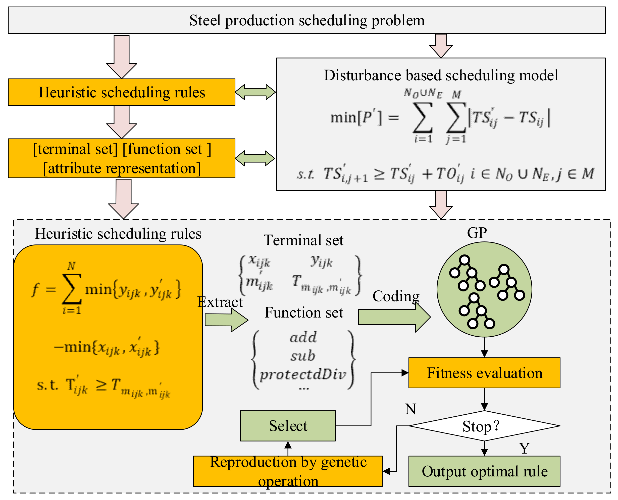
The scheduling plan can be adjusted through different scheduling rules for different disturbance events in steel production, including task disturbance, equipment disturbance, process disturbance, and time disturbance. Figure 7 shows the automatic generation framework of heuristic scheduling rules based on GP. After the disturbance event occurs, the system will generate an initial scheduling problem. For different scheduling problems and scheduling models, different heuristic scheduling rules and constraints will be generated. These scheduling rules and their constraints are connected and expressed by endpoint sets and function sets. After the model is generated, the population is initialized by GP, binary tree coding, the number of iterations is set, and the heuristic scheduling rules are decoded. After the decoding is completed, the optimal solution of the scheduling problem is generated by selecting, crossover, and mutation operations among the scheduling rules [33,34]. If the conditions are not met, continue to execute the loop program until the termination conditions are met, and the optimal rule is output.

In terms of fitness selection for GP, this paper adopts two different fitness methods: the least square fitness method, which is used to eliminate the difference between the output of the evolutionary target system and the output of the individual model. The other is structural fitness, which is used to limit the structural complexity of iterative individuals. The calculation of structural fitness requires repeated gene iterative operation, which is easy to produce a large number of individuals with a very complex structure, and the structural fitness needs to be optimized again. The fitness of the least square method represents the output error of the individual model, and the same input parameters are set for the individual evolutionary model and the optimization goal. Let the output of the individual evolutionary model be $y_{individual}\left(t\right)$, the output of the system is $y_{individual}\left(i\right)$, then the least-squares fitness is as shown in Equation (32).

$$f_{LS}={{\displaystyle \sum }}_{i=0}^M{\left(y_{individual}\left(t\right)-y_{individual}\left(i\right)\right)}^2$$

(32)

During the algorithm’s operation, each individual is sorted into the form of the simplest difference polynomial. If $Nt$ is the number of items contained in the simplest polynomial and $Ni$ is the maximum allowable number of items, the structural fitness is defined as Equation (33).

$$f_a=\left\{\frac{1.00\dots \dots Nt\le Ni}{10.0\dots \dots Nt\ge Ni}\right.$$

(33)

It can be seen that when the number of items of the simplest polynomial of the structural fitness function is less than or equal to the allowable number of items of its own polynomial, the structural fitness is similar to the least-squares fitness of the output error of the individual evolutionary model. When the number of items of the simplest polynomial of the structural fitness function is greater than the allowable number of polynomial items, the structural fitness is 10 times the least-squares fitness. At this time, the error is amplified by 10 times. Ensure that the size of individual evolutionary structure does not exceed the maximum range so that individuals within the range can evolve preferentially and eliminate evolutionary individuals beyond the maximum scope.

$$f_T=f_{LS}\times f_a$$

(34)

The combination of least squares fitness and structural fitness is an effective improvement of standard genetic programming algorithms. Combining the two fitness limits the unlimited reproduction of individual structures in the evolution process, reduces memory computing resources, solves the problem of time complexity, and effectively improves the operation efficiency of the algorithm.

The evaluation steps of the GP fitness function are as follows.

Step 1: Express the heuristic scheduling rules based on GP coding.

Step 2: Traverse the individual binary tree to obtain the general expression of heuristic scheduling rules.

Step 3: Through case matching, multiple disturbance rules are matched with the scheduling model to automatically generate the scheduling rules with the highest priority that meet different disturbance characteristics.

Step 4: Evaluate the fitness function of the obtained optimal scheduling rule. If it meets the performance requirements, it will be terminated. Otherwise, it will return to the genetic programming program and regenerate the scheduling rule that meets the conditions through genetic operation until the termination conditions are met.

4.6. The Solution Process Based on GP-HH

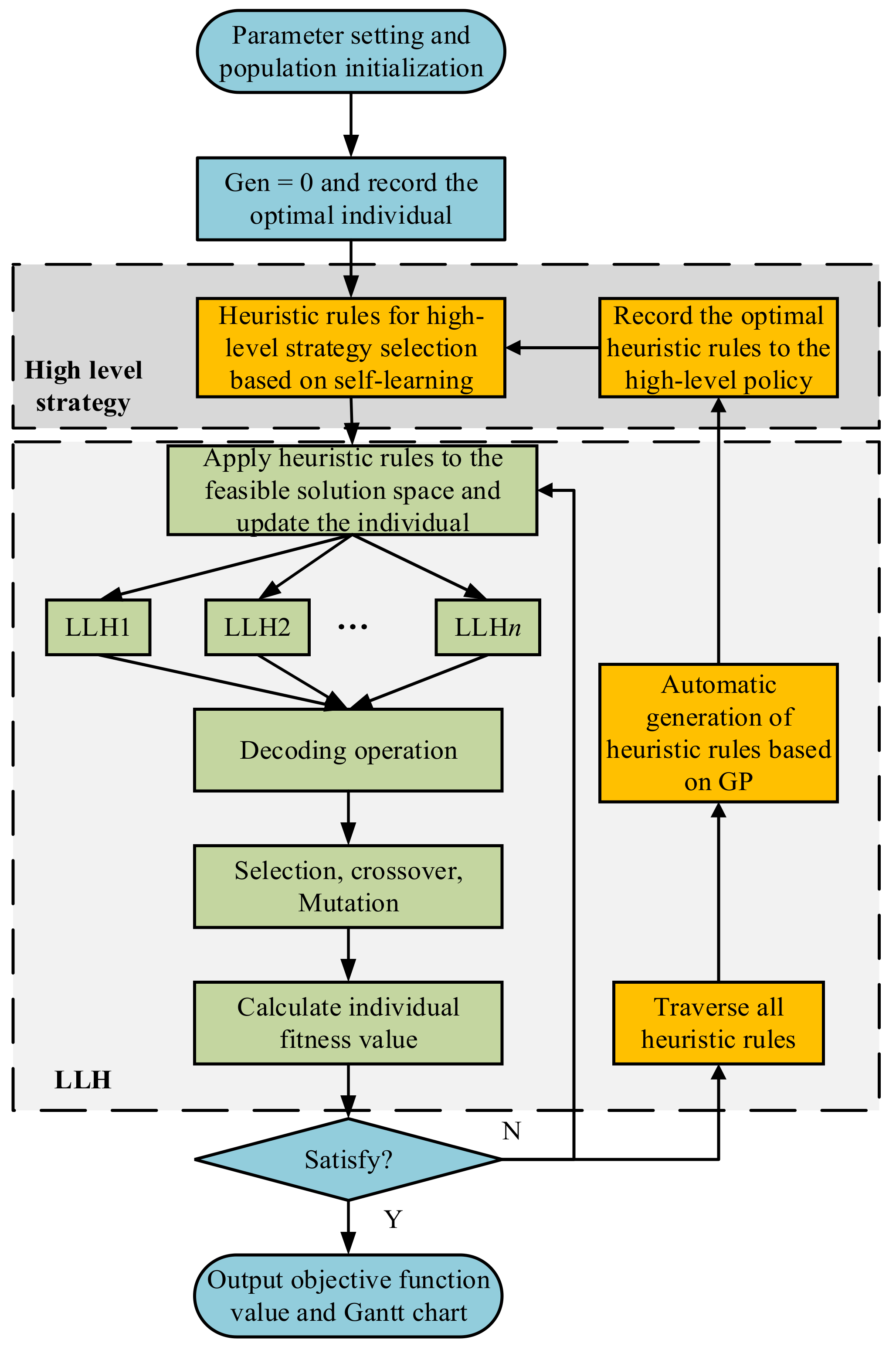
The algorithm process is shown in Figure 8. When the disturbance event occurs, the system automatically generates a production scheduling problem and judges whether to reschedule according to the scheduling problem. In rescheduling, a series of parameters of the scheduling model corresponding to the disturbance problem is set, and the initial solution is encoded. The LLH operator is applied to the feasible solution space. When the termination conditions are not met, and all heuristics cannot produce new solutions, based on traversing all LLH, the optimal scheduling rules are generated through GP-based automatic generation rules (selection, crossover, and mutation), which are recorded and used by high-level strategies. When the algorithm satisfies the iteration termination condition, the objective function value and Gantt chart are output.

5. Case Study

5.1. Original Steel Production Plan

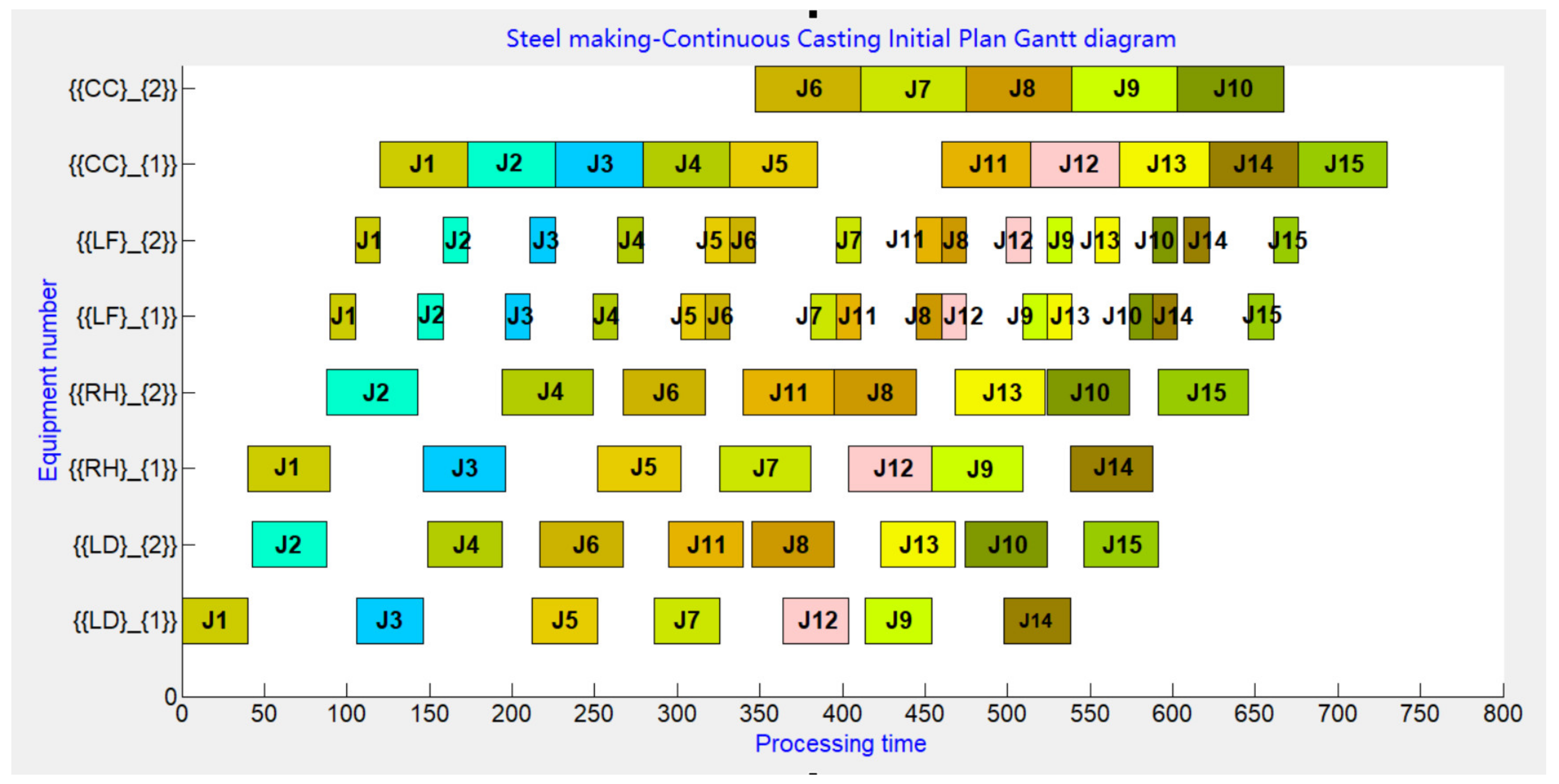
The actual production data from a steel plant are used for simulation verification to verify the algorithm’s effectiveness. The workshop includes the converter (LD) stage, RH parallel, LF serial double refining, and continuous casting. The specific equipment required is two converters (LD), two refining charges (RH), two LF charges, and two continuous casters (CC). The processing cases of three castings and fifteen charges are analyzed. The processing data of the charge at each stage are shown in

Table 3. Processing time of charge at each stage.

Casting	Charge	Processing Time
		LD1	LD2	RH1	RH2	LF1	LF2	CC1	CC2
1	5	40	45	50	55	15	15	53	61
2	5	40	50	55	50	15	15	57	64
3	5	40	45	50	55	15	15	54	63

LD: Linz Donawitz; RH: Ruhrstahl Hereaeus; LF:ladle furnace; CC: continuous casting.

.

The molten steel of fifteen charges is scheduled on the eight equipment and corresponding process constraints to generate a set of feasible actual production scheduling, including the processing time, start time, and end time of each charge in each equipment. The initial schedule is shown in

Table 4. Initial schedule plan.

	LD1	LD2	RH1	RH2	LF1	LF2	CC1	CC2
1–1	[0,40]		[40,90]		[90,105]	[105,120]	[125,173]
1–2		[43,88]		[88,143]	[143,158]	[158,173]	[173,226]
1–3	[106,146]		[146,196]		[196,211]	[211,226]	[226,279]
1–4		[149,194]		[194,249]	[249,264]	[264,279]	[279,332]
1–5	[212,252]		[252,302]		[302,317]	[317,332]	[332,385]
2–6		[217,267]		[267,317]	[317,332]	[332,347]		[347,411]
2–7	[286,326]		[326,381]		[381,396]	[396,411]		[411,475]
2–8		[345,395]		[395,445]	[445,460]	[460,475]		[475,539]
2–8	[414,454]		[454,509]		[509,524]	[524,539]		[539,603]
2–10		[474,524]		[524,574]	[574,588]	[588,603]		[603,667]
3–11		[295,340]		[340,395]	[396,445]	[445,460]	[460,514]
3–12	[364,404]		[404,454]		[460,499]	[499,514]	[514,568]
3–13		[423,468]		[468,523]	[524,553]	[553,568]	[568,622]
3–14	[498,538]		[538,588]		[588,607]	[607,622]	[622,676]
3–15		[546,591]		[591,646]	[646,661]	[661,676]	[676,730]

. The initial Gantt chart is shown in Figure 9.

5.2. Case Analysis

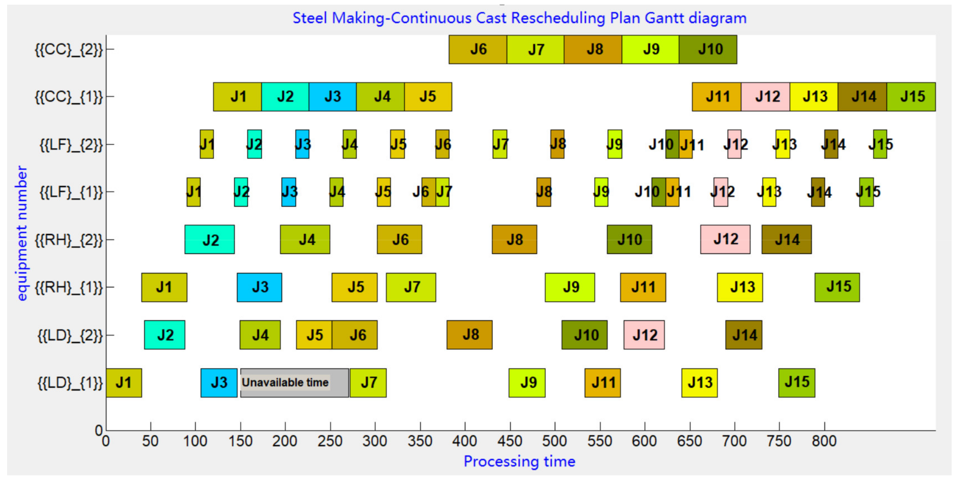
In case of equipment disturbance in SCC, the equipment failure will change processing time and directly affect the quality of products. Therefore, the objective function in this paper considers the shift in processing time when the total completion time and equipment assignment change, takes the difference of processing time before and after rescheduling as a critical reference index and takes the difference of equipment as an essential index. Set ${\omega }_1=0.6$, ${\omega }_2=0.4$, $minf={\omega }_1\times A_{ij}+{\omega }_2\times B_{ij}$. The maximum number of iterations is 350. The equipment disturbance parameter setting is shown in

Table 5. Equipment disturbance parameter setting.

Equipment	Disturbance	Start Time/Min	End Time/Min	Failure Time/Min
LD1	Equipment failure	150	270	120

. The failure equipment is LD1. The failure time starts at 150 min, end up in 270 min.

This experiment is programmed with Visual Studio C++ 2010. The running environment is Windows10, and the memory is 8 GB and CPU 2.6 GHz. Each case is run 10 times, and the results are averaged. Enable the scheduling model based on equipment disturbance and use GP–HH to solve the rescheduling plan. The rescheduling schedule plan is shown in

Table 6. Rescheduling schedule plan.

	LD1	LD2	RH1	RH2	LF1	LF2	CC1	CC2
1–1	[0,40]		[40,90]		[90,105]	[105,120]	[125,173]
1–2		[43,88]		[88,143]	[143,158]	[158,173]	[173,226]
1–3	[106,146]		[146,196]		[196,211]	[211,226]	[226,279]
1–4		[149,194]		[194,249]	[249,264]	[264,279]	[279,332]
1–5		[212,252]	[252,302]		[302,317]	[317,332]	[332,385]
2–6		[252,302]		[302,352]	[352,367]	[367,382]		[382,446]
2–7	[272,312]		[312,367]		[367,431]	[431,446]		[446,510]
2–8		[380,430]		[430,480]	[480,495]	[495,510]		[510,574]
2–9	[449,489]		[489,544]		[544,579]	[559,574]		[574,638]
2–10		[508,558]		[558,608]	[608,623]	[623,638]		[638,702]
3–11	[533,573]		[573,623]		[623,638]	[638,653]	[653,707]
3–12		[577,622]		[622,677]	[677,692]	[692,707]	[707,761]
3–13	[641,731]		[681,731]		[731,746]	[746,761]	[761,815]
3–14		[690,730]		[730,785]	[785,800]	[800,815]	[815,869]
3–15	[749,789]		[789,839]		[839,854]	[854,869]	[869,923]

. The rescheduling Gantt chart is shown in Figure 10.

To further verify the algorithm’s performance, according to the actual production data of field investigation, the fault equipment is set as LD1 in the steelmaking stage, the start time is 150 min, the end time is 270 min, and the duration is 120 min. The equipment disturbance rescheduling problems of different scales are solved respectively and shown in

Table 7. Experimental results at different scales.

Case	Casting	Charge	GP-HH
			Optimal Solution	Mean Value
1	3	15	3.693	3.696
2	8	26	6.153	6.158
3	13	57	7.238	7.239
4	18	68	7.605	7.606
5	22	83	7.884	7.885
6	28	120	7.849	7.851
7	35	147	7.953	7.955
8	46	212	7.962	7.965
9	55	282	7.863	7.866

.

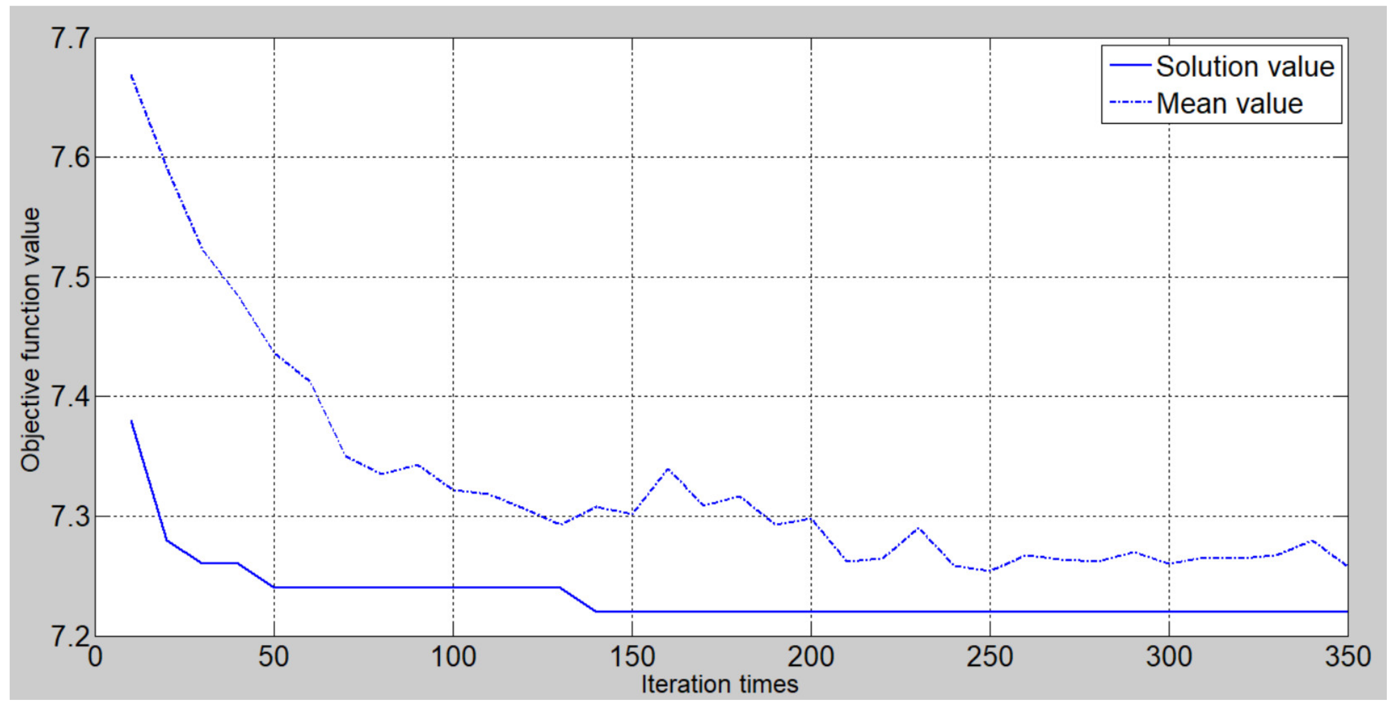
To verify the algorithm’s convergence, 13 castings and 57 charges were chosen as an example. The equipment failure time is still 150 min to 270 min, and LD1 is not available. As shown in Figure 11, in the iterative process of the objective function, the fitness function rapidly decreases to a lower level and then gradually converges, reflecting the advantages of the solution.

To further illustrate the effectiveness of GP-HH in solving the target model, the solution results are compared with the heuristic scheduling method [35]. The CPU running time is used as a reference to compare the performance of the algorithm comprehensively. The experimental results are shown in

Table 8. Comparison between GP-HH and heuristic scheduling methods.

Case	Casting	Charge	Heuristic Scheduling Method			GP-HH
			Optimal Solution	Mean Value	CUP Time/s	Optimal Solution	Mean Value	CUP Time/s
1	3	15	3.672	3.677	2.8	3.693	3.696	9.1
2	8	26	6.132	6.136	5.1	6.153	6.158	14.6
3	18	68	7.605	7.611	6.4	7.605	7.606	16.8
4	22	83	7.891	7.897	6.9	7.884	7.885	17.2
5	28	120	7.893	7.899	7.1	7.849	7.851	17.9
6	46	212	7.985	7.990	7.2	7.962	7.965	18.7

. GP-HH is more time-efficient than the heuristic scheduling method. In calculating small samples, GP cannot obtain enough samples for genetic operations such as crossover and mutation, and cannot obtain enough excellent heuristic scheduling rules, so GP-HH does not perform as well as the heuristic scheduling method in the optimal solution. However, in the comparative experiments of several cases, with the increase of the number of samples, the performance of GP-HH is gradually better than the heuristic scheduling method, and a better solution can be obtained in the effective time, which shows that GP-HH is effective to solve the steel production scheduling problem.

6. Conclusions

This paper proposes a steel production scheduling system architecture for CPS-oriented and studies a GP-HH algorithm to deal with different disturbance scenarios. Which can make up for the difficulty of dynamic scheduling in a complex environment and help steel production scheduling realize intelligent manufacturing. The main work is summarized as follows.

(1) A complete three-layer framework of steel production scheduling system for CPS-oriented is proposed, the differences between CPS and steel production scheduling system are analyzed, the characteristics, structure, and functions of steel CPS-oriented are redefined to integrate CPS with steel production scheduling system deeply is researched.

(2) Based on ontology, the concept and its core attributes of the production scheduling model of steel CPS are defined. The concept ontology of the steel CPS production scheduling model and the relationship framework between its attributes are proposed. The attributes represent the concept of the steel CPS scheduling model, and the relationship between core concepts is revealed, which lays a foundation for subsequent knowledge mining and knowledge scheduling.

(3) A hyper-heuristic algorithm of GP-HH is proposed. The framework of the algorithm and the composition of the heuristic scheduling method are described. A greedy strategy is used in the high-level domain to drive all bottom heuristic operators to fix the number. An automatic generation framework of heuristic scheduling rules based on GP is proposed to deal with different disturbance scenarios in the steel production scheduling environment. Finally, through a case study, the universality and effectiveness of the algorithm are verified.

However, these studies still need to be improved. Mining the association relationship between attributes of steel CPS production scheduling ontology model is still hard work. In addition, designing algorithms with better performance and more robustness is still the critical problem in the subsequent research.

References

- Long, J.Y.; Zheng, Z.; Gao, X.Q. Dynamic scheduling in steelmaking-continuous casting production for continuous caster breakdown. Int. J. Prod. Res. 2017, 55, 3197–3216. [Google Scholar] [CrossRef]
- Tang, L.; Meng, Y.; Chen, Z.-L.; Liu, J. Coil batching to improve productivity and energy utilization in steel production. MSom-Manuf. Serv. Oper. Manag. 2016, 18, 262–279. [Google Scholar] [CrossRef] [Green Version]
- Lin, D.Y.; Huang, T.Y. A Hybrid Metaheuristic for the Unrelated Parallel Machine Scheduling Problem. Mathematics 2021, 9, 768. [Google Scholar] [CrossRef]
- Liu, Y.; Peng, Y.; Wang, B.; Yao, S.; Liu, Z. Review on cyber-physical systems. IEEE/CAA J. Autom. Sin. 2017, 4, 27–40. [Google Scholar] [CrossRef]
- Guan, X.; Yang, B.; Chen, C.; Dai, W.; Wang, Y. A comprehensive overview of cyber-physical systems: From perspective of feedback system. IEEE/CAA J. Autom. Sin. 2016, 3, 1–14. [Google Scholar]
- Putnik, G.D.; Ferreira, L.; Lopes, N.; Putnik, Z. What is a cyber-physical system: Definitions and models spectrum. Fme Trans. 2019, 47, 663–674. [Google Scholar] [CrossRef]
- Zhou, J.; Zhou, Y.; Wang, B.; Zang, J. Human Cyber Physical Systems (HCPSs) in the context of new-generation intelligent manufacturing. Engineering 2019, 4, 624–636. [Google Scholar] [CrossRef]
- Keller, K.L. Leveraging biologically inspired models for cyber-physical systems analysis. IEEE Syst. J. 2018, 12, 3597–3607. [Google Scholar] [CrossRef]
- Graja, I.; Kallel, S.; Guermouche, N.; Cheikhrouhou, S.; Kacem, A.H. Modelling and verifying time-aware processes for cyber-physical environments. IET Softw. 2019, 13, 36–48. [Google Scholar] [CrossRef]
- Fu, Y.G.; Zhu, J.M.; Gao, S. CPS information security risk evaluation based on block chain and big data. Teh. Vjesn. Tech. Gaz. 2018, 25, 1843–1850. [Google Scholar]
- Mitsch, S.; Platzer, A. ModelPlex: Verified runtime validation of verified cyber-physical system models. Form. Methods Syst. Des. 2016, 49, 33–74. [Google Scholar] [CrossRef] [Green Version]
- Balasubramaniyan, S.; Srinivasan, S.; Buonopane, F.; Subathra, B.; Vain, J.; Ramaswamy, S. Design and verification of Cyber-Physical Systems using TrueTime evolutionary optimization and UPPAAL. Microprocess. Microsyst. 2016, 42, 37–48. [Google Scholar] [CrossRef]
- Zhang, Z.; Eyisi, E.; Koutsoukos, X.; Porter, J.; Karsai, G.; Sztipanovits, J. A co-simulation framework for design of time-triggered automotive cyber physical systems. Simul. Model. Pract. Theory 2014, 43, 16–33. [Google Scholar] [CrossRef] [Green Version]
- Jiménez-Martín, A.; Mateos, A.; Hernández, J.Z. Aluminium parts casting scheduling based on simulated annealing. Mathematics 2021, 9, 741. [Google Scholar] [CrossRef]
- Wang, H.-X.; Yan, H.-S. An interoperable adaptive scheduling strategy for knowledgeable manufacturing based on SMGWQ-learning. J. Intell. Manuf. 2016, 27, 1085–1095. [Google Scholar] [CrossRef]
- Yan, H.-S.; Li, W.-C. A scheduling procedure for a flow shop-like knowledgeable manufacturing cell with self-evolutionary features. Proc. Inst. Mech. Eng. Part B-J. Eng. Manuf. 2016, 230, 2296–2306. [Google Scholar] [CrossRef]
- Yan, H.-S.; Yang, H.-B. Deadlock-free scheduling of knowledgeable manufacturing cell with multiple machines and products. Proc. Inst. Mech. Eng. Part B-J. Eng. Manuf. 2015, 229, 1834–1847. [Google Scholar] [CrossRef]
- Jiang, G.; Chen, X.; Li, X.; Xiang, F.; Li, G. Model knowledge matching algorithm for steelmaking casting scheduling. Int. J. Wirel. Mob. Comput. 2018, 15, 215–222. [Google Scholar] [CrossRef]
- Chen, X.; Jiang, G.; Li, G.; Zuo, Y.; Xiang, F. A new knowledgeable encapsulation method of steel production scheduling model. Proc. Inst. Mech. Eng. Part B J. Eng. Manuf. 2020, 234, 1673–1685. [Google Scholar] [CrossRef]
- Xu, B.Z.; Wang, Y.; Ji, Z.C. Knowledge network model of the energy consumption in discrete manufacturing system. Mod. Phys. Lett. B 2017, 31, 19–21. [Google Scholar] [CrossRef] [Green Version]
- Drugan, M.M. Reinforcement learning versus evolutionary computation: A survey on hybrid algorithms. Swarm Evol. Comput. 2019, 44, 228–246. [Google Scholar] [CrossRef]
- Zhang, J.L.; Liu, J.L.; Zhao, Y.W.; Wang, H.W.; Leng, L.L.; Feng, Q.B. Hyper-heuristic for time-dependent VRP with simultaneous delivery and pick-up. Comput. Integr. Manuf. Syst. 2020, 26, 1905–1917. [Google Scholar]
- Asta, S.; Ozcan, E.; Curtois, T. A tensor based hyper-heuristic for nurse rostering. Knowl. Based Syst. 2016, 98, 185–199. [Google Scholar] [CrossRef] [Green Version]
- Choong, S.S.; Wong, L.P.; Lim, C.P. Automatic design of hyper-heuristic based on reinforcement learning. Inf. Sci. 2018, 436, 89–107. [Google Scholar] [CrossRef]
- Nasser RSabar, M.A.; Graham, K. A dynamic multi-armed bandit-gene expression programming hyper-heuristic for combinatorial optimization problems. IEEE Trans. Cybern. 2015, 45, 217–227. [Google Scholar]
- Lin, J.; Zhu, L.; Gao, K. A genetic programming hyper-heuristic approach for the multi-skill resource constrained project scheduling problem. Expert Syst. Appl. 2020, 140, 112915. [Google Scholar] [CrossRef]
- Kheiri, A.; Ozcan, E. Constructing constrained-version of magic squares using selection hyper-heuristics. Comput. J. 2014, 57, 469–479. [Google Scholar] [CrossRef] [Green Version]
- Yu, L.; Ma, H.; Wang, C. Research on construction of equipment phm knowledge ontology and semantic reasoning method. J. Ordnance Equip. Eng. 2019, 40, 126–130. [Google Scholar]
- Xiong, T.; Zhou, C.G.; Wang, M.Q. Rapid fire weapon technology knowledge push method based on manufacturing situation. J. Ordnance Equip. Eng. 2019, 40, 230–235. [Google Scholar]
- Yu, S.B.; Li, X.M.; Liu, D.; Cheng, J.B.; Li, Y.C. Study on equipment knowledge formalization description model based on extension theory. J. Ordnance Equip. Eng. 2016, 8, 23–28. [Google Scholar]
- Wang, J.H.; Chen, Y. Data-driven Job Shop production scheduling knowledge mining and optimization. Comput. Eng. Appl. 2018, 54, 264–270. [Google Scholar]
- Li, X.B.; Zhuang, P.J.; Yin, C. A metadata based manufacturing resource ontology modeling in cloud manufacturing systems. J. Ambient Intell. Humaniz. Comput. 2019, 10, 1039–1047. [Google Scholar] [CrossRef]
- Marko, D.; Domagoj, J.; Karlo, K. Adaptive scheduling on unrelated machines with genetic programming. Appl. Soft Comput. 2016, 48, 419–430. [Google Scholar]
- Nguyen, S.; Mei, Y.; Zhang, M. Genetic programming for production scheduling: A survey with a unified framework. Complex Intell Syst 2017, 3, 41–66. [Google Scholar] [CrossRef] [Green Version]
- Yu, S.P.; Chai, T.Y. Heuristic scheduling method for steelmaking and continuous casting production process. Control Theory Appl. 2016, 33, 1413–1421. [Google Scholar]
Figure 1.
The whole work in the paper.
Figure 2.
CPS architecture.