Research of Trajectory Optimization Approaches in Synthesized Optimal Control

Abstract

This article presents a study devoted to the emerging method of synthesized optimal control. This is a new type of control based on changing the position of a stable equilibrium point. The object stabilization system forces the object to move towards the equilibrium point, and by changing its position over time, it is possible to bring the object to the desired terminal state with the optimal value of the quality criterion. The implementation of such control requires the construction of two control contours. The first contour ensures the stability of the control object relative to some point in the state space. Methods of symbolic regression are applied for numerical synthesis of a stabilization system. The second contour provides optimal control of the stable equilibrium point position. The present paper provides a study of various approaches to find the optimal location of equilibrium points. A new problem statement with the search of function for optimal location of the equilibrium points in the second stage of the synthesized optimal control approach is formulated. Symbolic regression methods of solving the stated problem are discussed. In the presented numerical example, a piece-wise linear function is applied to approximate the location of equilibrium points.

1. Introduction

Russian neurophysiologist, Nobel laureate Ivan Pavlov in his Lectures on the work of the cerebral hemisphere [1] said: “Every material system can exist as an entity only so long as its internal forces of attraction, cohesion, etc., are equilibrated with the external forces influencing it. This applies in equal measure to such a simple object as a stone and to the most complex chemical substance, and it also holds good for the organism. As a definite material system complete in itself, the organism can exist only so long as it is in equilibrium with the environment”. Pavlov assumed that all complex physiological organisms aimed to balance external influences. In this regard, new modern computational methods can be considered to have emerged to counterbalance new complex computational problems.

The present work is devoted to the development and application of the synthesized optimal control method [2]. It was developed according to Pavlov’s paradigm for balancing the challenges of new complex control problems. It is a new approach to optimal control based on the control of the equilibrium point of a stabilized object. The approach is in two stages. Initially, a stabilization system is introduced into the control object, so the object obtains a special property—a special stable equilibrium point appears. It is known that the object possess good properties for control when its mathematical model in the phase space has a stable equilibrium point. The equilibrium point can be changed after some time, but the object, being stabilized, maintains equilibrium at each moment of time. Then, the object can be controlled by optimally changing the position of the stable equilibrium point.

The key stage of the considered approach is the solution of the control synthesis problem for constructing the stabilization system. The challenge is to find a mathematical expression for the control function. In the general case, this control function must have a special property: when it is inserted into the differential equations of the mathematical model of the control object, then a special stable equilibrium point appears in the space of solutions of these differential equations. All solutions of differential equations from a certain region of initial conditions will tend to this singular point of attraction.

Most of the known methods of control synthesis are associated with specifics of the model of the control object [3,4,5,6]; for example, analytical methods [7,8,9,10], as well as the use of various controllers [11,12,13]. However, there are now general numerical approaches to solve the synthesis problem based on application of symbolic regression methods [14,15,16,17,18,19]. These can be applied to find a solution without reference to specific model equations.

These methods belong to the class of machine learning control [20,21,22]. They allow automatically by means of computer searching for the desired mathematical expression in a coded form. When it comes to a machine search for mathematical expressions, it is usually assumed that the researcher firstly determines a structure of the mathematical expression accurate to parameters, and then the computer looks for the optimal values of these parameters in accordance with some given criterion. Popular neural networks [23,24,25,26,27] are also used for these purposes. In this respect, neural networks are also functions of a given structure, in which it is necessary to find the optimal values of a large number of parameters. Symbolic regression methods, in contrast to neural networks, allow to search for the optimal structure of the desired function together with the optimal parameters of this function. In this context, this approach is more unambiguous and universal. Moreover, the received function is described in a way which is understandable to a researcher, not a black box as in the case with neural networks. It can be said that symbolic regression is a generalization of neural networks. Therefore, all analytical problems, where solutions must be obtained in the form of functions, can now be solved automatically by computers. Nonlinear and differential equations, integrals, inverse functions and other problems can now be solved by numerical symbolic regression methods.

Thus, symbolic regression methods allow a mathematical expression describing the stabilization system that ensures the presence of an equilibrium point in the state space to be found. According to the approach, the synthesized function includes a set of parameters that affect the position of the equilibrium point. Optimal control is realized by changing the position of the equilibrium point. In previous works on synthesized optimal control [2,28], the theoretical foundations of the method were presented and comparative estimates with other known approaches to solving the optimal control problem were given. The emphasis was placed on the substantiation of an approach to control based on the equilibrium point and on the numerical solution of the synthesis problem based on symbolic regression methods. One of the main features of the synthesized approach is in practical feasibility of the received numerical solutions of the optimal control problem for complex systems. In applied devices, the control system requires additional adjustments because there are always some differences between real control systems and analytical solutions made using models of the control objects. Thus, to implement analytical solutions into practice, it is necessary to construct additional stabilization systems, which modify the object model as a whole, significantly complicating it. As a result, analytical trajectories are no longer optimal. The synthesized solution can be implemented to the object without additional construction of a stabilization system.

In the present paper, the research of the synthesized optimal control approach is aimed at studying ways to control equilibrium points. Particularly, this can be just a set of points. In the general case, the vector of parameters that effect the positions of equilibrium points can be considered as some function. In this work, the problem statement of optimal movement according to a set of equilibrium points is presented (Section 2), methods for solving the stated problem are proposed (Section 3 and Section 4) and a computational example (Section 5) is provided to demonstrate how the approach performs the task with piece-wise linear functions defining the positions of the equilibrium points.

2. Problem of Optimal Movement on Trajectory Determined by a Set of Points

The mathematical model of a control object is given in the form of the ordinary differential equation system

$$\dot{\mathbf{x}}=\mathbf{f}(\mathbf{x},\mathbf{u}),$$

(1)

where $\mathbf{x}\in {\mathbb{R}}^n$, $\mathbf{u}\in \mathrm{U}\subseteq {\mathbb{R}}^m$, $\mathrm{U}$ is a compact set, $m\le n$.

Given initial conditions

$$\mathbf{x}\left(0\right)={\mathbf{x}}^0.$$

(2)

The ordered set of points is given

$$\mathrm{Y}=({\mathbf{y}}^{*,1},\dots ,{\mathbf{y}}^{*,N}),$$

(3)

where $\mathbf{y}\in {\mathbb{R}}^l$, $l\le n$.

The formulas of transformation from state space vector $\mathbf{x}$ to the vector $\mathbf{y}$ are determined

$$\mathbf{y}=\mathbf{w}\left(\mathbf{x}\right),$$

(4)

where

$$\mathbf{w}\left(\mathbf{x}\right):{\mathbb{R}}^n\to {\mathbb{R}}^l.$$

(5)

The control is to be found in the form

$$\mathbf{u}=\mathbf{v}\left(t\right)\in \mathrm{U}$$

(6)

to deliver minimum to the functional

$$J=t_f+a_1\sum _{k=1}^N\underset{t}{min}\parallel {\mathbf{y}}^{*,k}-\mathbf{w}\left(\mathbf{x}\left(t\right)\right)\parallel \to \underset{\mathbf{u}\in \mathrm{U}}{min},$$

(7)

where $t_f$ is a finishing time,

$$t_f=\left\{\begin{array}{c}t,\mathrm{if}t<t^{+}\mathrm{and}\parallel {\mathbf{y}}^{*,N}-\mathbf{w}\left(\mathbf{x}\left(t\right)\right)\parallel \le \epsilon \hfill \\ t^{+},\mathrm{otherwise}\hfill \end{array}\right.,$$

(8)

$a_1$ is a weight coefficient, $t^{+}$ and $\epsilon$ are given positive numbers.

To solve this problem (1)–(8), the control function can be found as

$$\mathbf{u}=\mathbf{h}\left(\mathbf{g}\right(k,t)-\mathbf{w}(\mathbf{x}\left(t\right)\left)\right)\in \mathrm{U},$$

(9)

where

$$\mathbf{g}(k,t)=\left\{\begin{array}{c}{\mathbf{y}}^{*,k},\mathrm{if}(t-t_{k-1}<\mathsf{\Delta })\wedge (\parallel {\mathbf{y}}^{*,k}-\mathbf{w}\left(\mathbf{x}\right(t\left)\right)\parallel >{\epsilon }_1)\hfill \\ k\leftarrow k+1,t_k\leftarrow t,\mathrm{otherwise}\hfill \end{array}\right.,$$

(10)

$k=1,\dots ,N-1$, $t_0=0$, $\mathbf{g}(N,t)={\mathbf{y}}^{*,N}$, $\mathsf{\Delta }$ and ${\epsilon }_1$ are given small positive numbers.

3. Synthesized Optimal Control

For solution of the problem (1)–(8), the synthesized optimal control approach was used. According to the approach, firstly, it is necessary to solve the control synthesis problem and to provide existence of a stable equilibrium point in the phase space of differential Equation (1). For this purpose, the control function with the following properties must be found

$$\mathbf{u}=\mathbf{g}({\mathbf{x}}^{*}-\mathbf{x}),$$

(11)

where ${\mathbf{x}}^{*}$ is a constant vector, ${\mathbf{x}}^{*}={[x_1^{*}\dots x_n^{*}]}^T$. The function is such that if it is inserted into right side of differential Equations (1), there is an equilibrium point in the state space

$$\tilde{\mathbf{x}}\left({\tilde{x}}^{*}\right)\in {\mathbb{R}}^n$$

(12)

$$\mathbf{f}(\tilde{\mathbf{x}}\left({\tilde{x}}^{*}\right),\mathbf{g}(\tilde{\mathbf{x}}-{\mathbf{x}}^{*}))=0,$$

(13)

$$det(\lambda \mathbf{E}-\mathbf{A})={\lambda }^n+b_{n-1}{\lambda }^{n-1}+\dots +b_1\lambda +b_0=\prod _{j=1}^n(\lambda -{\lambda }_j)=0,$$

(14)

$${\lambda }_j={\alpha }_j+i{\beta }_j,j=1,\dots ,n,$$

(15)

where

$${\alpha }_j<0,j=1\dots ,n,$$

(16)

$$i=\sqrt{-1},$$

$$\mathbf{A}=\frac{\partial \mathbf{f}(\tilde{\mathbf{x}}\left({\mathbf{x}}^{*}\right),\mathbf{g}({\mathbf{x}}^{*}-\tilde{\mathbf{x}}\left({\mathbf{x}}^{*}\right)))}{\partial \mathbf{x}},$$

(17)

$\mathbf{E}$ is $n\times n$ unit matrix.

In the result of the synthesis problem solution, a new mathematical model of control object is obtained

$$\dot{\mathbf{x}}=\mathbf{f}(\mathbf{x},\mathbf{g}({\mathbf{x}}^{*}-\mathbf{x})).$$

(18)

In this model (18), there is a new control vector ${\mathbf{x}}^{*}$. This vector ${\mathbf{x}}^{*}$ has the same dimension n as the main state space vector $\mathbf{x}$. There is a domain of values

$${\mathbf{x}}^{*}\in {\mathrm{X}}^{*}\subseteq {\mathbb{R}}^n$$

(19)

where the system (18) always has a stable equilibrium point $\tilde{\mathbf{x}}\left({\mathbf{x}}^{*}\right)$ in the phase space. Therefore, the system (18) is controlled by changing the position of the equilibrium point.

Now, in the second stage of the synthesized optimal control approach, it is necessary to find a control function in the form

$${\mathbf{x}}^{*}=\mathbf{v}\left(t\right)$$

(20)

for optimization of criterion (7).

The found control can be implemented directly in the on-board computer of the control object. Here, it is not necessary to design a stabilization system for movement of the control object in an optimal trajectory.

When solving the control synthesis problem, the given trajectory (3) is not taken into account; therefore, in the second stage, the optimal control problem can be solved for any given trajectory.

4. Numerical Methods

4.1. Methods for the Control Synthesis Problem

The control synthesis problem is the most difficult with regard to realization of the synthesized optimal control. In control theory, for the synthesis problem, different analytical methods are used. These are backstepping integrator [8], design of aggregated controller [9], synthesis on the base of Lyapunov functions [10] and others. All analytical methods are not universal as they are connected with the mathematical model of the control object. Technical methods have the same disadvantages [11]. To insert a controller in the control object, it is necessary to know which control vector component affects which state vector component. Transformation of the mathematical model to the linear equation system can be made correctly only for stable system in neighborhood of a stable equilibrium point.

In the synthesized optimal control approach, to solve the control synthesis problem, machine learning control by symbolic regression is applied. These methods code the mathematical expression on the base of elementary functions sets and search the optimal code of mathematical expression by a special genetic algorithm.

Symbolic regression learning of control is a universal numerical tool for the synthesis problem and it is independent of the mathematical model of the control object. However, the application of symbolic regression methods is very difficult since the search for the function must be carried out in a space where there is no metric. Furthermore, there are only a few research groups in the world dealing with this issue. The majority uses genetic programming [16,17,20,29,30,31]. It codes a mathematical expression in the form of a computing tree and presents this code in the form of an array in computer memory. GP has a computational drawback that consists of the fact that different mathematical expressions have codes of different lengths. There are many other symbolic regression methods that have fixed lengths of code, such as Cartesian genetic programming [32], network operator [33] and complete binary analytic programming [34]. In the application example of the present paper, the method of the network operator was applied. It is based on the principle of small variations of the basic solution [35]. The main idea of the principle is that the search for a function begins not with a random possible solution, but with some given possible solution, which is called the basic solution. The basic solution can also be random if there is no preliminary data on the desired function. However, if the developer has some experience or intuition, then he can put them in the description of the basic solution. The application of this principle helps to significantly narrow the search space and overcome the mentioned difficulty of search space complexity, which allows for the synthesis problems to be solved in a reasonable time.

To solve the control synthesis problem, it is necessary for the mathematical model of the control object (1) to give a set of initial conditions

$${\mathrm{X}}_0=\{{\mathbf{x}}^{0,1},\dots ,{\mathbf{x}}^{0,K}\}\subseteq {\mathbb{R}}^n,$$

(21)

and one terminal condition

$${\mathbf{x}}^{*}\in {\mathbb{R}}^n.$$

(22)

The found optimal control function (11) has to satisfy the optimal value of the criterion

$$J_s=max\{t_{f,i}:i=1,\dots ,K\}\to min,$$

(23)

where $t_{f,i}$ is the time it takes to achieve the terminal condition (22) from the initial condition ${\mathbf{x}}^{0,i}$, $i=1,\dots ,K$,

$$t_{f,i}=\left\{\begin{array}{c}t,\mathrm{if}t<t^{+}\mathrm{and}\parallel {\mathbf{x}}^{*}-\mathbf{x}(t,{\mathbf{x}}^{0,i})\parallel \le {\epsilon }_0\hfill \\ t^{+},\mathrm{otherwise}\hfill \end{array}\right.,$$

(24)

$\mathbf{x}(t,{\mathbf{x}}^{0,i})$ is a partial solution of the differential equation system (1) from the initial condition ${\mathbf{x}}^{0,i}$, $i\in \{1,\dots ,K\}$.

When solving the control synthesis problem (1), (21)–(24) every control function (11) is inserted into the right part of the mathematical model (18) in the form of a special symbolic regression code. For calculation of the criterion (23), a special algorithm calculates a value of control by the code of control function (11).

4.2. Methods for the Optimal Control Problem

The formal mathematical statement for the optimal control problem in the second stage consists of that for the mathematical model of the control object (18). It is necessary to find control in the form (20) in order to provide the optimal value of the quality criterion (7).

For numerical solution of the optimal control problem, the axis of time was divided into some intervals. In each interval, the control function (20) is approximated as a function of time defined with accuracy to values of some parameters. This allows for the transformation of the optimal control problem from infinite dimension optimization to a nonlinear programming problem in the space with finite dimension. The dimension of the search space is equal to a number of parameters in each interval multiplied by the number of intervals. For example, if the control function is approximated in each interval as a piece-wise linear function, then a number of parameters is equal to the number of intervals plus one. The piece-wise linear control function (20) has the following form

$$x_i^{*}=q_{k+(i-1)d}+(q_{k+(i-1)d+1}-q_{k+(i-1)d})\frac{t-k\mathsf{\Delta }t}{\mathsf{\Delta }t},$$

(25)

where $\mathbf{q}={[q_1\dots q_{dn}]}^T$ is the vector of searched parameters, k is the interval number, $k\mathsf{\Delta }t\le t<(k+1)\mathsf{\Delta }t$, $\mathsf{\Delta }t$ is a time interval, d is a number of interval boundaries, $k=1,\dots ,d-1$, $i=1,\dots ,n$.

To solve the optimization problem, various numerical methods of optimization can be used. However, many studies have shown [36,37,38,39] that the most effective methods for solving the problem are evolutionary algorithms, in so as far as, generally, the objective functional could be not unimodal.

5. Computational Example

As an example, consider the problem of optimal control for one mobile robot following the given trajectories.

The mathematical model of a robot has the following form

$$\begin{array}{ccc}\hfill {\dot{x}}_1& =& 0.5(u_1+u_2)cos\left(x_3\right),\hfill \\ \hfill {\dot{x}}_2& =& 0.5(u_1+u_2)sin\left(x_3\right),\hfill \\ \hfill {\dot{x}}_3& =& 0.5(u_1-u_2),\hfill \end{array}$$

(26)

where $\mathbf{x}={\left[x_1{x}_2{x}_3\right]}^T$ is a vector of state space, $\mathbf{u}={\left[u_1{u}_2\right]}^T$ is a control vector.

Restrictions on control are given

$$-10\le u_i\le 10,i=1,2.$$

(27)

Initial conditions are set

$$x_i\left(0\right)=0,i=1,2,3.$$

(28)

The program trajectory is given as an ordered set of $N=40$ points

$$\mathrm{Y}=({\mathbf{y}}^{*,1}={\left[y_1^{*,1}{x}_2^{*,1}{y}_3^{*,1}\right]}^T,\dots ,{\mathbf{y}}^{*,40}={\left[y_1^{*,40}{y}_2^{*,40}{y}_3^{*,40}\right]}^T).$$

(29)

In this example, spaces ${\mathbb{R}}^l$ and ${\mathbb{R}}^n$ coincide

$$\mathbf{y}=\left[\begin{array}{c}{y}_1\\ y_2\\ y_3\end{array}\right]=\mathbf{w}\left(\mathbf{x}\right)=\left[\begin{array}{ccc}1& 0& 0\\ 0& 1& 0\\ 0& 0& 1\end{array}\right]\left[\begin{array}{c}{x}_1\\ x_2\\ x_3\end{array}\right].$$

(30)

In the first stage, the synthesis problem (1), (21)–(24) was solved. For the solution, the network operator method was used. As a result, the following control function was received

$$u_i=\left\{\begin{array}{c}10,\mathrm{if}{\tilde{u}}_i>10\hfill \\ -10,\mathrm{if}{\tilde{u}}_i<-10\hfill \\ {\tilde{u}}_i,\mathrm{otherwise}\hfill \end{array}\right.,i=1,2,$$

(31)

where

$${\tilde{u}}_1={\rho }_{16}\left(A\right)+\mathrm{sgn}(x_3^{*}-x_3)+{\rho }_{19}\left(r_3(x_3^{*}-x_3)\right)+\sqrt[3]{D}+{({\rho }_{23}\left(A\right)+D)}^{-1},$$

(32)

$${\tilde{u}}_2={\rho }_{23}(sin(x_1^{*}-x_1)+{\rho }_{19}\left(r_2(x_2^{*}-x_2)\right)+tanh\left(r_1(x_1^{*}-x_1)\right)+r_2(x_2^{*}-x_2)+r_3(x_3^{*}-x_3))+$$

$${\tilde{u}}_1+\mathrm{sgn}(x_1^{*}-x_1)+{\rho }_{16}\left(A\right)+arctan\left(B\right)+sin\left(E\right),$$

(33)

$$A=x_1^{*}-x_1+tanh(tanh\left(r_1(x_1^{*}-x_1)\right)+r_2(x_2^{*}-x_2)\mathrm{sgn}(x_1^{*}-x_1)+r_3(x_3^{*}-x_3))+$$

$$sin(x_1^{*}-x_1)+{\rho }_{19}\left(r_2(x_2^{*}-x{+}_2)\right)+tanh\left(r_1(x_1^{*}-x_1)\right)+r_2(x_2^{*}-x_2)\mathrm{sgn}(x_1^{*}-x_1)+r_3(x_3^{*}-x_3),$$

(34)

$$B={\rho }_{19}\left(r_2(x_2^{*}-x_2)\mathrm{sgn}(x_1^{*}-x_1)\right)+tanh\left(r_1(x_1^{*}-x_1)\right)+r_2(x_2^{*}-x_2)\mathrm{sgn}(x_1^{*}-x_1)+r_3(x_3^{*}-x_3))+$$

$$arctan\left(r_1(x_1^{*}-x_1)\right)+{\rho }_4(sin(x_1^{*}-x_1)+\mathrm{sgn}\left(A\right)+\sqrt[3]{\sqrt[3]{x_1^{*}-x_1}+A}+$$

$${\rho }_4\left(r_1(x_1^{*}-x_1)\right)+tanh\left(z_7\right)+r_2(x_2^{*}-x_2)\mathrm{sgn}(x_1^{*}-x_1)+r_3(x_3^{*}-x_3)+\mathrm{sgn}\left(z_{12}\right)+\sqrt[3]{x_1^{*}-x_1}+A,$$

(35)

$$C={\rho }_9(x_3^{*}-x_3)+arctan\left(r_1\right)+\mathrm{sgn}\left(r_1(x_1^{*}-x_1)\right)+{\rho }_{23}(sin(x_1^{*}-x_1)+B+$$

$${\rho }_{19}\left(r_2(x_2^{*}-x_2)\mathrm{sgn}(x_1^{*}-x_1)\right)+tanh\left(r_1(x_1^{*}-x_1)\right)+r_2(x_2^{*}-x_2)\mathrm{sgn}(x_1^{*}-x_1)+r_3(x_3^{*}-x_3)),$$

(36)

$$D=sin\left(r_3(x_3^{*}-x_3)\right)+sin(x_1^{*}-x_1)+{\rho }_{19}(r_2(x_2^{*}-x_2)\mathrm{sgn}(x_1^{*}-x_1)+tanh\left(r_1(x_1^{*}-x_1)\right)+$$

$$r_2(x_2^{*}-x_2)\mathrm{sgn}(x_1^{*}-x_1)+r_3(x_3^{*}-x_3)+{\left(\sqrt[3]{x_1^{*}-x_1}+A\right)}^3+tanh\left(C\right),$$

(37)

$$\begin{gathered} E={\rho }_{16}\left(A\right)+\mathrm{sgn}(x_3^{*}-x_3)+{\rho }_{19}\left(r_3(x_3^{*}-x_3)\right)+\sqrt[3]{D}+{({\rho }_{23}\left(A\right)+D)}^{-1} \\ {\rho }_{16}\left(z\right)=\left\{\begin{array}{c}z,\mathrm{if}\left|z\right|<1\hfill \\ \mathrm{sgn}\left(z\right),\mathrm{otherwise}\hfill \end{array}\right.,{\rho }_{19}\left(z\right)=\mathrm{sgn}\left(z\right)exp(-|z\left|\right), \\ {\rho }_{23}\left(z\right)=z-z^3,{\rho }_4\left(z\right)=\mathrm{sgn}\left(z\right)\sqrt{\left|z\right|},{\rho }_9\left(z\right)=\left\{\begin{array}{c}1,\mathrm{if}z>0\hfill \\ 0,\mathrm{otherwise}\hfill \end{array}\right., \\ {r}_1=14.72876r_2=2.02710r_3=4.02222z_9=r_3{x}_3{z}_{10}={\rho }_8\left(z_7\right)+z_8+z_9{z}_{11}= \\ {\rho }_{12}\left(x_1\right)+{\rho }_{19}\left(z_8\right)+z_{10}{z}_{12}=x_1+{\rho }_8\left(z_{10}\right)+z_{11}{z}_{13}={\rho }_{15}\left(x_1\right)+z_{12}{z}_{14}={\rho }_4\left(z_7\right)+z_{10}+ \\ {\rho }_{10}\left(z_{12}\right)+z_{13}{z}_{15}={\rho }_{13}\left(z_7\right)+{\rho }_4\left(z_{11}\right)+{\rho }_{10}\left(z_{12}\right)+{\rho }_{15}\left(z_{13}\right)+z_{14}{z}_{16}={\rho }_9\left(x_3\right)+{\rho }_{13}\left(r_1\right)+ \\ {\rho }_{10}\left(z_7\right)+{\rho }_{23}\left(z_{11}\right)+z_{15}{z}_{17}={\rho }_{12}\left(z_9\right)+z_{11}+{\rho }_{14}\left(z_{13}\right)+{\rho }_8\left(z_{16}\right)z_{18}=z_{17}{z}_{19}=z_{18},z_{20}= \\ {\rho }_{23}\left(z_{12}\right)+z_{19}{z}_{21}={\rho }_{10}\left(x_3\right)+{\rho }_{19}\left(z_9\right)+{\rho }_{15}\left(z_{18}\right)+{\rho }_5\left(z_{20}\right)z_{22}={\rho }_{16}\left(z_{12}\right)+z_{21}{u}_1=z_{22}{u}_2= \\ {\rho }_{10}\left(x_1\right)+{\rho }_{23}\left(z_{11}\right)+{\rho }_{16}(z_{12}+{\rho }_{13}\left(z_{15}\right)+{\rho }_{12}\left(z_{22}\right)+u_1 \end{gathered}$$

(38)

In the second stage, the optimal control problem (7), (18), (20) was solved. The control function was searched in the form (25).

In the first experiment, the goal trajectory describes function sinus on the plane $\{x_1;x_2\}$

$$y_i^{*,1}=0,i=1,2,3$$

(39)

$$y_1^{*,j}=y_1^{*,j-1}+{\mathsf{\Delta }}_1,j=2,\dots ,40,$$

(40)

$$y_2^{*,j}=10sin\left(\frac{y_1^{*,j}\pi }{10}\right),j=2,\dots ,40,$$

(41)

$$y_3^{*,j}=arctan\left(\frac{y_2^{*,j}-y_2^{*,j-1}}{{\mathsf{\Delta }}_1}\right),j=2,\dots ,40.$$

(42)

where ${\mathsf{\Delta }}_1=0.5$.

In the search, the following values of parameters were used: $\mathsf{\Delta }t=0.28$, $t^{+}=5.6$. In total, there were 20 intervals and $d=21$ parameters for each component. To find vector a with 63 components, $\mathbf{q}={[q_1\dots q_{63}]}^T$. The parameters had the following constraints

$$\begin{array}{c}-2\le q_{1+3k}\le 22\\ -12\le q_{2+3k}\le 12\\ -0.5\pi \le q_{3+3k}\le 0.5\pi \end{array},k=1,\dots ,21.$$

(43)

To solve the problem particle swarm optimization [40] (PSO) algorithm was applied.

As a result, the following solution was found:

$$\begin{array}{ccc}\hfill \mathbf{q}& =& [18.07416.83818.1211.38818.37911.76811.51319.3126.471220.68612.36716.460\hfill \\ \hfill & & 14.28021.86921.99921.97421.20421.99421.99222.00022.00010.438-4.645\hfill \\ \hfill & & 3.8478.7182.9885.6095.4623.9564.437-3.9600.784-0.185-7.510-10.515\hfill \\ \hfill & & -9.344-\mathrm{9.5199.0666.529}-2.842-2.623-1.674-0.4871.2361.547-0.310\hfill \\ \hfill & & 1.09020.514-0.0150.005-0.4920.801-0.651-1.5350.8811.099-0.505\hfill \\ \hfill & & {-0.2721.3791.5670.8941.4041.547]}^T\hfill \end{array}$$

(44)

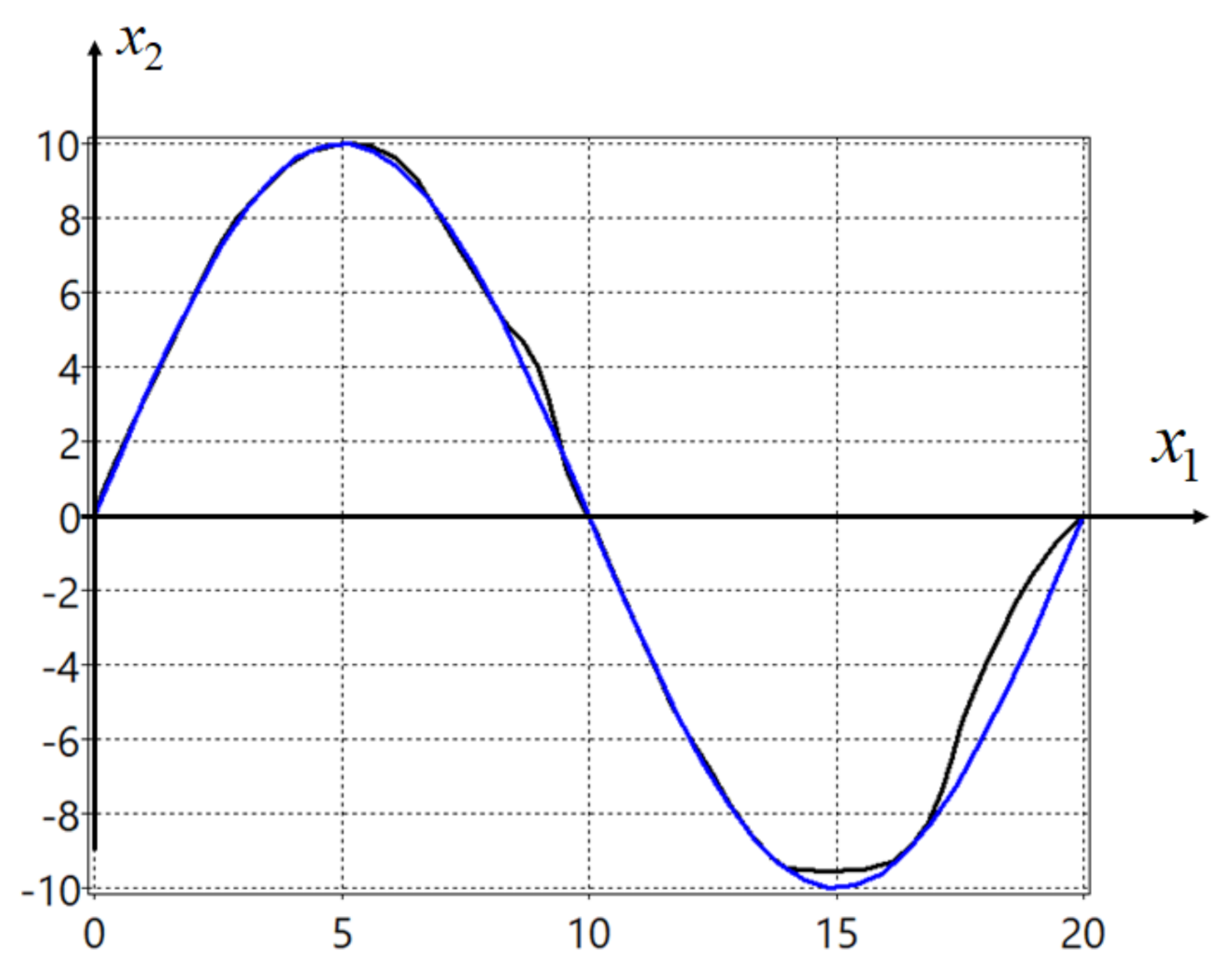
The value of functional (7) is $J=6.4004$. In Figure 1 projections of trajectories on the plane $\{x_1;x_2\}$ are presented. In the Figure 1 blue line is the given trajectory, black line is the trajectory of mobile robot with found optimal control.

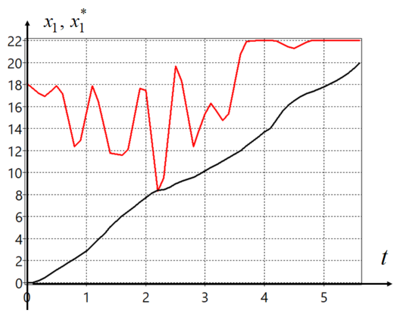
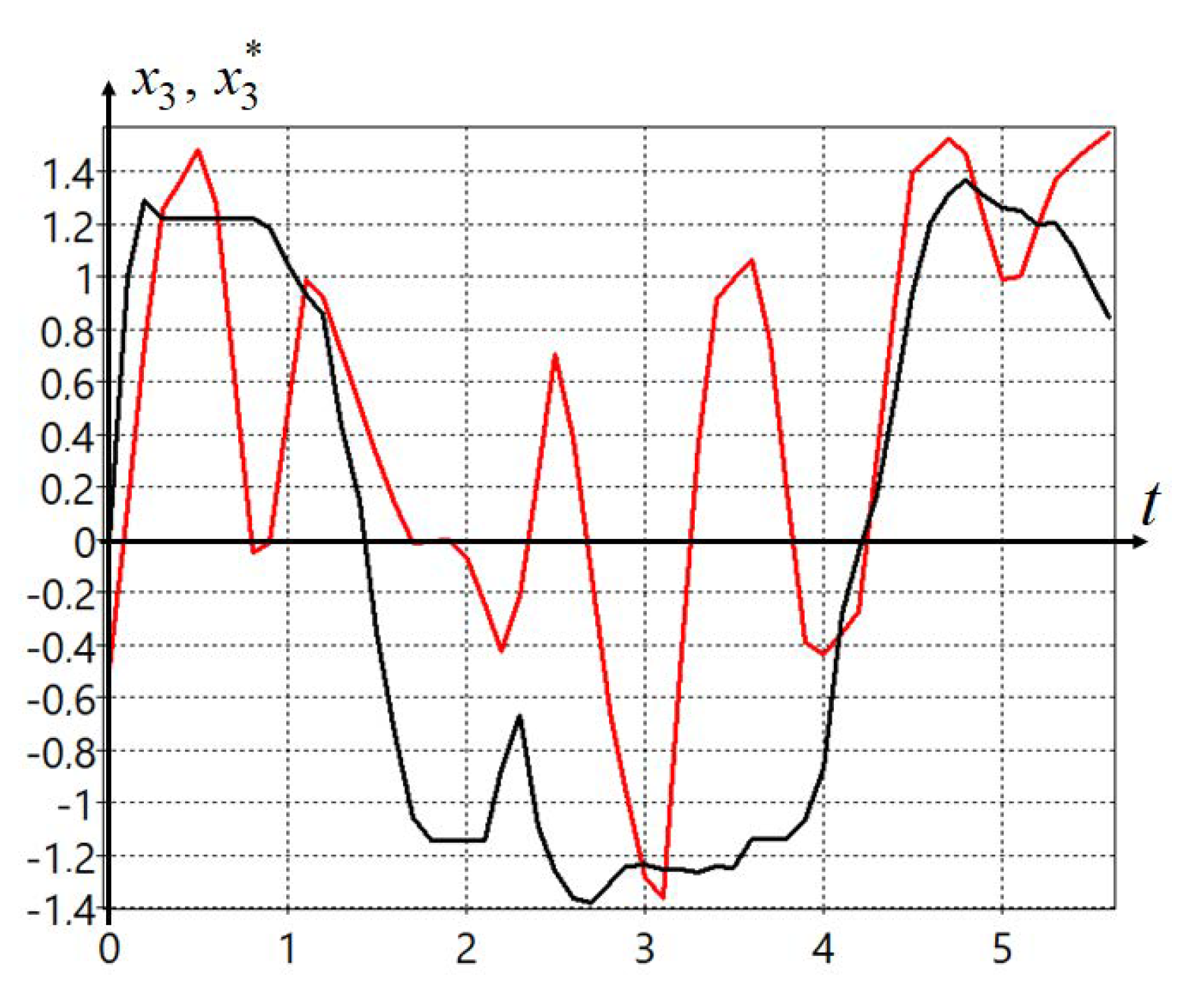
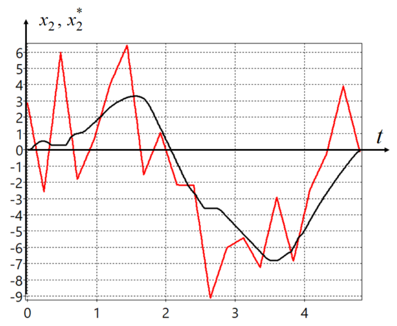
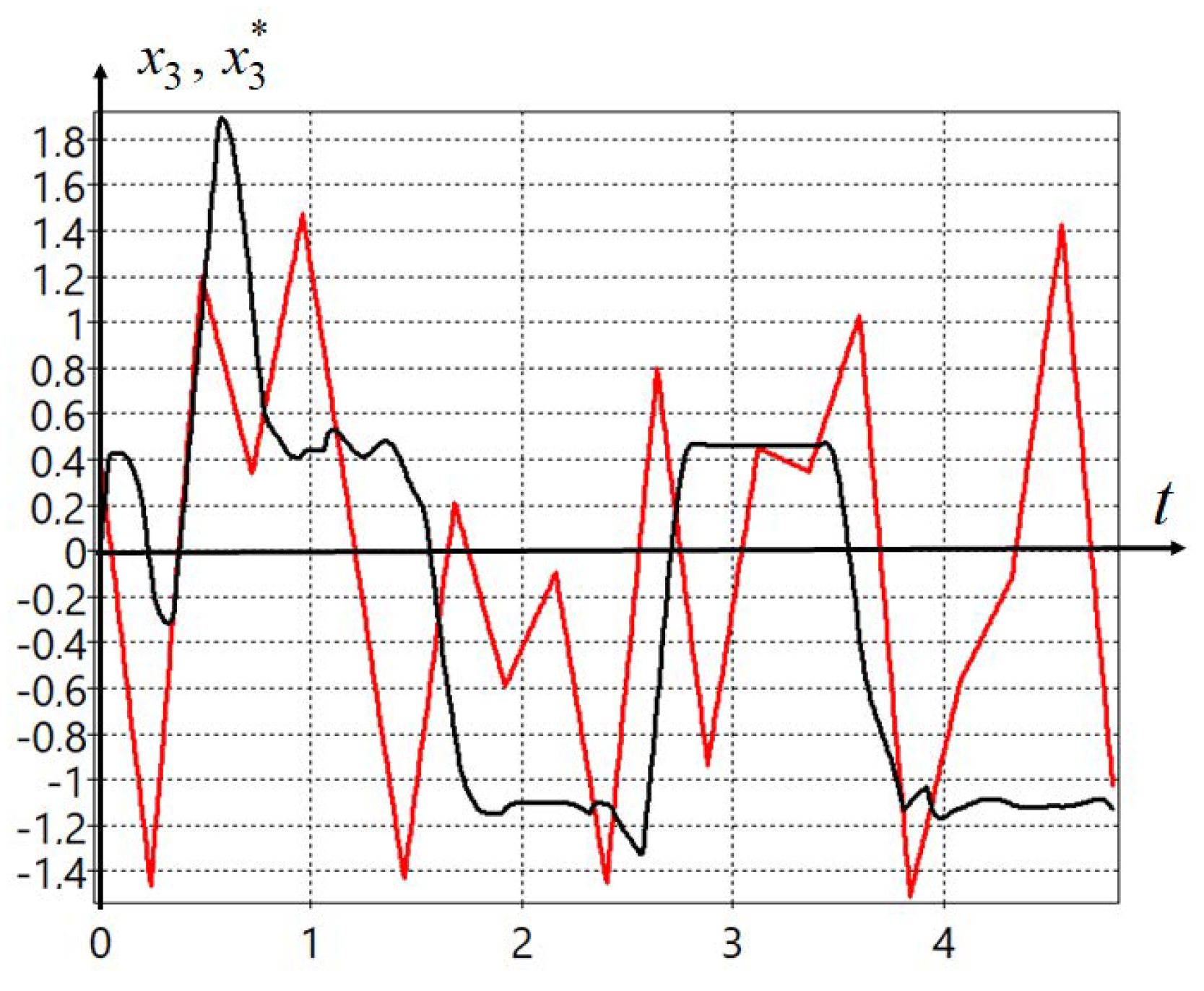
In Figure 2, Figure 3 and Figure 4 plots of optimal trajectories $x_i\left(t\right)$, $i=1,2,3$ (black lines) and optimal controls $x_i^{*}\left(t\right)$, $i=1,2,3$ (red lines) are presented.

As seen from the plots, optimal trajectories and their goal control trajectory of the position of equilibrium points do not coincide. According to synthesized control, the vector ${\mathbf{x}}^{*}\left(t\right)$ in control function (25) determines the position of a stable equilibrium point in the current moment, t. However, according to the criterion (7) the control object should strive to reach ordered points on the trajectory as quickly as possible, so the control point ${\mathbf{x}}^{*}$ should be located behind the point on the trajectory. The control object must not stop at the trajectory point, and it must go through it or near it. The object moves more slowly near the equilibrium point than far from it. Therefore, this is the reason why the equilibrium points trajectory coincides with the trajectory of the object movement.

In the second experiment, the trajectory in the form of a square was considered. The points were defined by the following Equations (39) and

$$y_1^{*,i}=y_1^{*,i-1}+{\mathsf{\Delta }}_2,i=2,\dots ,11,$$

(45)

$$y_2^{*,i}=0.5y_1^{*,i},i=2,\dots ,11,$$

(46)

$$y_3^{*,i}=arctan\left(\frac{y_2^{*,i}-y_2^{*,i-1}}{{\mathsf{\Delta }}_2}\right),i=2,\dots ,11,$$

(47)

where ${\mathsf{\Delta }}_2=0.7$,

$$y_1^{*,i}=y_1^{*,i-1}+{\mathsf{\Delta }}_3,i=12,\dots ,21,$$

(48)

$$y_2^{*,i}=-2y_1^{*,i}+17.5,i=12,\dots ,21,$$

(49)

$$y_3^{*,i}=arctan\left(\frac{y_2^{*,i}-y_2^{*,i-1}}{{\mathsf{\Delta }}_3}\right),i=12,\dots ,21,$$

(50)

where ${\mathsf{\Delta }}_3=0.35$,

$$y_1^{*,i}=y_1^{*,i-1}+{\mathsf{\Delta }}_4,i=22,\dots ,31,$$

(51)

$$y_2^{*,i}=0.5y_1^{*,i}-8.75,i=22,\dots ,31,$$

(52)

$$y_3^{*,i}=arctan\left(\frac{y_2^{*,i}-y_2^{*,i-1}}{{\mathsf{\Delta }}_4}\right),i=22,\dots ,31,$$

(53)

where ${\mathsf{\Delta }}_4=-0.7$,

$$y_1^{*,i}=y_1^{*,i-1}+{\mathsf{\Delta }}_5,i=32,\dots ,41,$$

(54)

$$y_2^{*,i}=-2y_1^{*,i},i=32,\dots ,41,$$

(55)

$$y_3^{*,i}=arctan\left(\frac{y_2^{*,i}-y_2^{*,i-1}}{{\mathsf{\Delta }}_5}\right),i=32,\dots ,41,$$

(56)

where ${\mathsf{\Delta }}_5=-0.35$,

The optimal control problem had the following parameters $t^{+}=4.8$, $\mathsf{\Delta }t=2.4$. The vector of parameters included 63 components. The constraints on the parameters were

$$\begin{array}{c}-2\le q_{1+3k}\le 15\\ -12\le q_{2+3k}\le 8\\ -0.5\pi \le q_{3+3k}\le 0.5\pi \end{array},k=1,\dots ,21.$$

(57)

Particle swarm optimization [40] (PSO) algorithm was used for the solution.

The optimal values of parameters were

$$\begin{array}{ccc}\hfill \mathbf{q}& =& [11.71312.04911.0752.2167.7299.3786.72312.24914.71414.39512.6299.562\hfill \\ \hfill & & -0.576-1.997-1.9980.1800.832-1.976-1.860-1.963-1.9632.887\hfill \\ \hfill & & -2.5935.988-1.8030.5934.0896.419-1.5261.047-2.163-2.196-9.116\hfill \\ \hfill & & -6.031-5.418-7.228-2.923-6.839-2.463-0.2553.917-0.131\hfill \\ \hfill & & 0.403-1.4611.2000.3381.4710.053-1.4310.213-0.591-0.096-1.451\hfill \\ \hfill & & {0.7988-0.9340.4510.3481.0291-1.512-0.566-0.1251.424-1.025]}^T.\hfill \end{array}$$

(58)

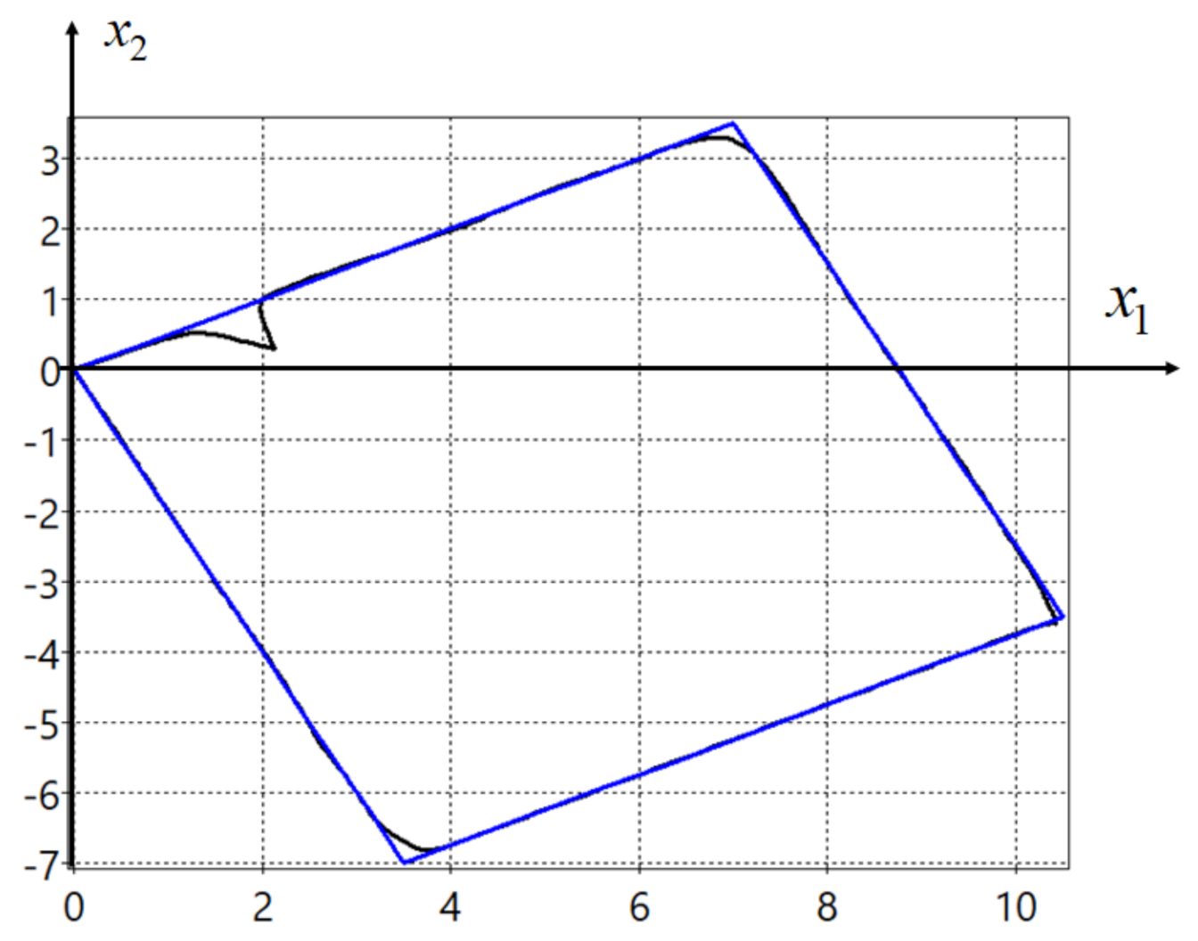
The value of the functional (7) was $5.0544$. Projections on the horizontal plane $\{x_1;x_2\}$ of given (blue lines) and found (black lines) trajectories are presented in Figure 5.

Plots of optimal trajectories and controls are presented in Figure 6, Figure 7 and Figure 8.

As can be seen from the graphs, the obtained control based on the synthesized optimal control allows for the problem to be solved with a given accuracy. In Figure 6, Figure 7 and Figure 8, the effect of non-coincidence of the trajectories of the equilibrium points and the trajectories of the object’s movement is also observed, which is quite understandable, as in the first example, in view of the presence of a performance criterion in the functional.

6. Conclusions

The optimal control problem of movement along a given trajectory determined in the form of a points set is considered. The quality criterion consists of trajectory travel time and accuracy. To solve the problem, the synthesized optimal control was used. The main advantage of the solution achieved using this approach is that it can be realized on the on-board computer without additional construction of a stabilization system. According to synthesized optimal control, firstly the control synthesis problem is solved and then a control is performed by changing equilibrium point location. The position of the equilibrium point is defined by some parametric vector, which corresponds to the state vector. In this work, for the first time—in contrast to other works devoted to the synthesized approach—an optimal function of time is used to control the equilibrium point position. In the experiment, two different trajectories for a mobile robot consisting of forty points were considered. For the control synthesis problem, a machine learning control method of the network operator was applied. Computational experiments have shown that the found optimal trajectories of the parametric vector do not coincide with the points of the trajectory, but the control object moves along the given trajectory fast enough and with a high accuracy.

Thus, we have demonstrated that the synthesized optimal control method is a mathematical approach to solve the optimal control problem in terms of the quality functional. The approach is quite universal as it is not tied to specific properties of the control object model or a type of trajectory, nor does it require manual selection of control channels or selection and adjustment of controllers. The development of the control system occurs automatically using modern computational machine learning methods.

References

- Pavlov, I. Experimental Psychology and Other Essays; Philosophical Library: New York, NY, USA, 1957. [Google Scholar]
- Diveev, A.; Shmalko, E.; Serebrenny, V.; Zentay, P. Fundamentals of Synthesized Optimal Control. Mathematics 2021, 9, 21. [Google Scholar] [CrossRef]
- Liu, P.; Yu, H.; Cang, S. Trajectory Synthesis and Optimization of an Underactuated Microrobotic System with Dynamic Constraints and Couplings. Int. J. Control. Autom. Syst. 2018, 16, 2373–2383. [Google Scholar] [CrossRef]
- Matschek, J.; Bäthge, T.; Faulwasser, T.; Findeisen, R. Nonlinear predictive control for trajectory tracking and path following: An introduction and perspective. In Handbook of Model Predictive Control; Birkhäuser: Cham, Switzerland, 2019; pp. 169–198. [Google Scholar]
- Chen, H.; Mitra, S. Synthesis and verification of motor-transmission shift controller for electric vehicles. In Proceedings of the 2014 ACM/IEEE International Conference on Cyber-Physical Systems, ICCPS 2014, Art. No. 6843708, Berlin, Germany, 14–17 April 2014; pp. 25–35. [Google Scholar]
- Merkulov, V.I. Algorithm synthesis of the trajectory control of a mobile bistatic system of command radio control. Radiotekhnika 1998, 4, 99–101. [Google Scholar]
- Aguilar, C.O.; Krener, A.J. Numerical Solutions to the Bellman Equation of Optimal Control. J. Optim. Theory Appl. 2014, 160, 527–552. [Google Scholar] [CrossRef]
- Luo, Y.; Zhao, S.; Zhang, H. A New Robust Adaptive Neural Network Backstepping Control for Single Machine In finite Power System With TCSC. IEEE/CAA J. Autom. Sin. 2020, 7, 48–56. [Google Scholar]
- Kolesnikov, A.A.; Kolesnikov, A.A.; Kuz’menko, A.A. Backstepping and ADAR Method in the Problems of Synthesis of the Nonlinear Control Systems. Mekhatronika Avtom. Upr. 2016, 17, 435–445. (In Russian) [Google Scholar] [CrossRef] [Green Version]
- Nersesov, S.G.; Haddad, W.M. On the Stability and Control of Nonlinear Dynamical Systems via Vector Lyapunov Functions. IEEE Trans. Autom. Contr. 2006, 51, 203–215. [Google Scholar] [CrossRef]
- Åström, K.; Hägglund, T. PID Controllers: Theory, Design and Tuning; Instrument Society of America: Research Triangle Park, NC, USA, 1995. [Google Scholar]
- Yang, J.; Lu, W.; Liu, W. PID Controller Based on the Artificial Neural Network. In Advances in Neural Networks, Lecture Notes in Computer Science; Yin, F.L., Wang, J., Guo, C., Eds.; Springer: Berlin/Heidelberg, Germany, 2004; Volume 3174. [Google Scholar]
- Wang, L.-X. Stable Adaptive Fuzzy Control of Nonlinear Systems. IEEE Trans. Fuzzy Syst. 1993, 1, 146–155. [Google Scholar] [CrossRef]
- Freitas, A. Data Mining and Knowledge Discovery with Evolutionary Algorightms; Springer: Berlin/Heidelberg, Germany, 2002. [Google Scholar]
- Winkler, S. Evolutionary System Identification—Modern Concepts and Practical Applications. In Reihe C—Technik und Naturwissenschaften; Trauner: Linz, Austria, 2008. [Google Scholar]
- Alibekov, E.; Kubalık, J.; Babushka, R. Symbolic method for deriving policy in reinforcement learning. In Proceedings of the 55th IEEE Conference on Decision and Control (CDC), Las Vegas, NV, USA, 12–14 December 2016; pp. 2789–2795. [Google Scholar]
- Derner, E.; Kubalík, J.; Babushka, R. Reinforcement Learning with Symbolic Input–Output Models. In Proceedings of the 2018 IEEE/RSJ International Conference on Intelligent Robots and Systems (IROS), Madrid, Spain, 1–5 October 2018; pp. 3004–3009. [Google Scholar]
- Diveev, A.I.; Shmalko, E.Y. Automatic Synthesis of Control for Multi-Agent Systems with Dynamic Constraints. IFAC-PapersOnLine 2015, 48, 384–389. [Google Scholar] [CrossRef]
- Diveev, A.; Shmalko, E. Machine-made Synthesis of Stabilization System by Modified Cartesian Genetic Programming. IEEE Trans. Cybern. 2020. in print. [Google Scholar]
- Duriez, T.; Brunton, S.L.; Noack, B.R. Machine Learning Control—Taming Nonlinear Dynamics and Turbulence; Springer: Cham, Switzerland, 2017. [Google Scholar]
- Diveev, A.; Konstantinov, S.; Shmalko, E.; Dong, G. Machine Learning Control Based on Approximation of Optimal Trajectories. Mathematics 2021, 9, 265. [Google Scholar] [CrossRef]
- Upadhyay, D.; Schaal, C. Optimizing the driving trajectories for guided ultrasonic wave excitation using iterative learning control. Mech. Syst. Signal Process. 2020, 144, 106876. [Google Scholar] [CrossRef]
- Persio, L.D.; Garbelli, M. Deep Learning and Mean-Field Games: A Stochastic Optimal Control Perspective. Symmetry 2021, 13, 14. [Google Scholar] [CrossRef]
- He, W.; Huang, Y.; Fu, Z.; Lin, Y. ICONet: A Lightweight Network with Greater Environmental Adaptivity. Symmetry 2020, 12, 2119. [Google Scholar] [CrossRef]
- Sutton, R.S.; Barto, A.G. Reinforcement Learning: An Introduction; MIT Press: Cambridge, MA, USA, 1998. [Google Scholar]
- Martens, J. Deep learning via hessian-free optimization. In Proceedings of the 27th International Conference on Machine Learning, Haifa, Isreal, 21–24 June 2010. [Google Scholar]
- Witten, I.H.; Frank, E. Data Mining: Practical Machine Learning Tools and Techniques, 2nd ed.; Morgan Kaufman—Elsevier: Amsterdam, The Netherlands, 2005. [Google Scholar]
- Diveev, A.; Shmalko, E. Optimal Feedback Control through Numerical Synthesis of Stabilization System. In Proceedings of the 7th International Conference on Control, Decision and Information Technologies, CoDIT 2020, Prague, Czech Republic, 29 June–2 July 2020; pp. 112–117. [Google Scholar]
- Koza, J.R. Genetic Programming: On the Programming of Computers by Means of Natural Selection; MIT Press: Cambridge, MA, USA; London, UK, 1992. [Google Scholar]
- Yang, G.; Jeong, Y.; Min, K.; Lee, J.-W.; Lee, B. Applying Genetic Programming with Similar Bug Fix Information to Automatic Fault Repair. Symmetry 2018, 10, 92. [Google Scholar] [CrossRef] [Green Version]
- Dracopoulos, D.C.; Kent, S. Genetic programming for prediction and control. Neural Comput. Appl. 1997, 6, 214–228. [Google Scholar] [CrossRef] [Green Version]
- Miller, J.F. Cartesian Genetic Programming; Springer: Berlin/Heidelberg, Germany, 2011; 342p, ISBN 978-3-642-17310-3. [Google Scholar]
- Diveev, A.I.; Shmalko, E.Y. Self-adjusting control for multi robot team by the network operator method. In Proceedings of the 2015 European Control Conference, Linz, Austria, 15–17 July 2015; pp. 709–714. [Google Scholar]
- Diveev, A.I.; Shmalko, E.Y. Complete binary variational analytic programming for synthesis of control at dynamic constraints. In Proceedings of the ITM Web of Conferences, Moscow, Russia, 14–15 February 2017; Volume 10. [Google Scholar]
- Diveev, A. Small Variations of Basic Solution Method for Non-numerical Optimization. IFAC-PapersOnLine 2015, 48, 28–33. [Google Scholar] [CrossRef]
- Andrzej, O.; Stanislaw, K. Evolutionary Algorithms for Global Optimization. In Global Optimization. Nonconvex Optimization and Its Applications; Pintér, J.D., Ed.; Springer: Boston, MA, USA, 2006; Volume 85. [Google Scholar]
- Diveev, A.I.; Konstantinov, S.V. Study of the practical convergence of evolutionary algorithms for the optimal program control of a wheeled robot. J. Comput. Syst. Sci. Int. 2018, 57, 561–580. [Google Scholar] [CrossRef]
- Michalewicz, Z. Genetic Algorithms, Numerical Optimization, and Constraints. In Proceedings of the Sixth International Conference on Genetic Algorithms, Pittsburgh, PA, USA, 15–19 July 1995; pp. 151–158. [Google Scholar]
- Homaifar, A.; Qi, C.; Lai, S. Constrained optimization via genetic algorithms. Simulation 1994, 62, 242–254. [Google Scholar] [CrossRef]
- Kennedy, J.; Eberhart, R. Particle swarm optimization. In Proceedings of the IEEE International Conference on Neural Networks IV, Perth, Australia, 27 November–1 December 1995; pp. 1942–1948. [Google Scholar]
Figure 1.
Projections of the given and found trajectories on the horizontal plane.
Figure 2.
Optimal trajectory (black) and optimal control (red).
Figure 3.
Figure 4.
Figure 5.
Projections of trajectories on the horizontal plane.
Figure 6.
Optimal trajectory (black) and optimal control (red) for movement on square.
Figure 7.
Figure 8.
Publisher’s Note: MDPI stays neutral with regard to jurisdictional claims in published maps and institutional affiliations. |
© 2021 by the authors. Licensee MDPI, Basel, Switzerland. This article is an open access article distributed under the terms and conditions of the Creative Commons Attribution (CC BY) license (http://creativecommons.org/licenses/by/4.0/).
Share and Cite
MDPI and ACS Style
Diveev, A.; Shmalko, E. Research of Trajectory Optimization Approaches in Synthesized Optimal Control. Symmetry 2021, 13, 336. https://doi.org/10.3390/sym13020336
AMA Style
Diveev A, Shmalko E. Research of Trajectory Optimization Approaches in Synthesized Optimal Control. Symmetry. 2021; 13(2):336. https://doi.org/10.3390/sym13020336
Chicago/Turabian StyleDiveev, Askhat, and Elizaveta Shmalko. 2021. "Research of Trajectory Optimization Approaches in Synthesized Optimal Control" Symmetry 13, no. 2: 336. https://doi.org/10.3390/sym13020336
Note that from the first issue of 2016, this journal uses article numbers instead of page numbers. See further details here.