Article

Monitoring Hydrological Patterns of Temporary Lakes Using Remote Sensing and Machine Learning Models: Case Study of La Mancha Húmeda Biosphere Reserve in Central Spain

by
Carolina Doña
1,
Ni-Bin Chang
2,
Vicente Caselles
1,
Juan Manuel Sánchez
3,
Lluís Pérez-Planells
1,
Maria Del Mar Bisquert
3,
Vicente García-Santos
1,
Sanaz Imen
2 and
Antonio Camacho
4,*
1
Department of Earth Physics and Thermodynamics, University of Valencia, Burjassot, 46100 Valencia, Spain
2
Department of Civil, Environmental, and Construction Engineering, University of Central Florida, Orlando, 32816 FL, USA
3
Department of Applied Physics, University of Castilla-La Mancha, 16071 Cuenca, Spain
4
Cavanilles Institute of Biodiversity and Evolutionary Biology, University of Valencia, Burjassot, 46100 Valencia, Spain
*
Author to whom correspondence should be addressed.
Remote Sens. 2016, 8(8), 618; https://doi.org/10.3390/rs8080618
Submission received: 29 February 2016 / Revised: 4 July 2016 / Accepted: 21 July 2016 / Published: 26 July 2016
(This article belongs to the Special Issue What can Remote Sensing Do for the Conservation of Wetlands?)

Abstract

:
The Biosphere Reserve of La Mancha Húmeda is a wetland-rich area located in central Spain. This reserve comprises a set of temporary lakes, often saline, where water level fluctuates seasonally. Water inflows come mainly from direct precipitation and runoff of small lake watersheds. Most of these lakes lack surface outlets and behave as endorheic systems, where water withdrawal is mainly due to evaporation, causing salt accumulation in the lake beds. Remote sensing was used to estimate the temporal variation of the flooded area in these lakes and their associated hydrological patterns related to the seasonality of precipitation and evapotranspiration. Landsat 7 ETM+ satellite images for the reference period 2013–2015 were jointly used with ground-truth datasets. Several inverse modeling methods, such as two-band and multispectral indices, single-band threshold, classification methods, artificial neural network, support vector machine and genetic programming, were applied to retrieve information on the variation of the flooded areas. Results were compared to ground-truth data, and the classification errors were evaluated by means of the kappa coefficient. Comparative analyses demonstrated that the genetic programming approach yielded the best results, with a kappa value of 0.98 and a total error of omission-commission of 2%. The dependence of the variations in the water-covered area on precipitation and evaporation was also investigated. The results show the potential of the tested techniques to monitor the hydrological patterns of temporary lakes in semiarid areas, which might be useful for management strategy-linked lake conservation and specifically to accomplish the goals of both the European Water Framework Directive and the Habitats Directive.

Graphical Abstract

1. Introduction

Wetlands contribute a wealth of ecosystem services, including the regulation of the hydrological cycle for flood and drought control, and provide water supply, wildlife refuges, aesthetic enjoyment and recreational opportunities, among others. According to the Ramsar Convention, wetlands, in a broad sense, include all lakes and rivers, underground aquifers, swamps and marshes, wet grasslands, peatlands, oases, estuaries, deltas and tidal flats, mangroves and other coastal areas, coral reefs and all constructed sites, such as fish ponds, rice paddies, reservoirs and salt pans. Although these areas have a critical value to sustainable development, they are detrimentally impacted by urban growth, agricultural land reclamation and derived pollution [1].
The Biosphere Reserve of La Mancha Húmeda is currently the main wetland area in the Iberian Peninsula. This Lake District is one of the wetland complexes most threatened by anthropogenic activity, mainly by groundwater overexploitation due to excessive use for irrigated agriculture. This area is an important refuge for endangered waterfowl species, following the protection criteria for birds in Europe, and also holds endangered habitats [2]. Because of its natural and ethnographic values, it was designated a Biosphere Reserve.
The water balance and hydrological variations are intimately tied to potential changes in a lentic ecosystem. Understanding the dynamics of water in lakes helps the goal of conservation and recovery of these valuable ecosystems [3]. This is especially relevant given several environmental initiatives, such as the European Water Framework Directive (WFD), which came into force in 2000, and the Habitats Directive, delivered in 1992. These directives require each member state in the European Union to achieve a good ecological/conservation status for their water bodies and associated habitats and species, forcing the establishment of conservation actions. Previously, these critical areas in Spain were identified and studied using maps, field campaigns [4] and photo interpretation techniques. To enhance these systematic efforts, remote sensing technologies facilitate the content-based mapping over space and time, leading to multitemporal change detection of the hydrological variations in wetlands. Mapping surface water bodies allows for the investigation of water balance dynamics by providing information on the temporal and spatial variations of surface water coverage, this being especially relevant under the current climate change scenario. In the last few years, some published studies focused on finding a holistic approach to estimate the occurrence of water pixels with several satellite remote sensing imageries. These studies can be classified as based on: (1) single-band threshold; (2) image transformation; (3) two-band spectral indices (vegetation + water indices); (4) two-band spectral water indices; and (5) thematic classification methods.
The earliest related study, published in 1976 [5], identified ponds and lakes using single-band or combinations of bands from Landsat 1 and was followed by additional studies. To delineate open water body features, McFeeters [6] proposed the Normalized Difference Water Index (NDWI), developed using the green and Near Infrared (NIR) bands of the Thematic Mapper sensor (TM) onboard Landsat 4 and 5. Positive values of this index correspond to water pixels in the image. A modified NDWI with the aid of NIR and Short Wave Infrared (SWIR) bands was also proposed by Gao [7] to study liquid water in vegetation; later, Xu [8] proposed an additional modification to the NDWI including green and SWIR bands to study open water features. Several researchers used these indices in conjunction with Landsat, Quickbird or SPOT-4 imageries to estimate the water surface of lakes [9,10], deltas or river basins [11,12,13], the extents of seasonal and permanent waters in arid areas [14] and coast lines [15]. Extended studies covered different indices with the aid of several satellite imageries, such as Landsat 7-ETM+ (Enhanced Thematic Mapper Plus), SPOT (Satellites Pour l’ Observation de la Terre or Earth-observing Satellites), ASTER (Advanced Spaceborne Thermal Emission and Reflection Radiometer) and MODIS (Moderate-resolution Imaging Spectroradiometer) [16].
Several comparisons among indices designed to estimate water pixels from remote sensing images have been recently published, including those comparing the NDWIs [14], other using density slicing of single bands and the Tasseled Cap Wetness (TCW) [17,18], as well as comparisons using a variants of the Principal Component Analysis (PCA) to estimate open water extent with TERRA/ASTER and Landsat imagery [19]. A Linear Discriminant Analysis Water Index (LDAWI) composed of the green, red, NIR and SWIR bands of SPOT-5 images to map lake surface [20] has also been used to compare in water indices. Furthermore, classic thematic classification methods have been used, such as the maximum likelihood method used to map surface water in a wetland [21,22], the NIR single-band method, a pixel-based method, the object-based segmentation band [23] and the Automated Water Extraction Index (AWEI) [24]. Furthermore, several researchers applied single-band thresholds, such as the NIR band based on the Advanced Very High Resolution Radiometer (AVHRR) and MODIS sensors, to map seasonal inland waters in Central Asia [25] and to estimate the water surface of Sub-Saharan West-African wetlands [26], respectively.
Some methods applied to wetland monitoring combined the NIR band to estimate the water pixels and the NDVI to study wetland vegetation [26], as well as the spectral analytical process and Band 5 of Thematic Mapper [27]. The objectives of our study were to: (1) investigate the applicability of some of the previously-tested methods to estimate the water pixels in our study area and to compare them with the genetic algorithm approach; (2) develop a systematic methodology to monitor the changes in the water cover in several temporary lakes located in the Biosphere Reserve of La Mancha Húmeda (Spain) using Landsat 7-ETM+ imagery; and (3) investigate the interplay between precipitation, evaporation and the subsequent changes of water-covered area in these lakes to unveil the seasonal effect. Our findings elucidate the hydrological patterns of these lakes and provide tools to improve the management policies for lake protection, conservation and ecosystem recovery under the European Water Framework Directive and the Habitats Directive in semiarid areas heavily experiencing the effects of climate change.

2. Materials and Methods

2.1. Study Area

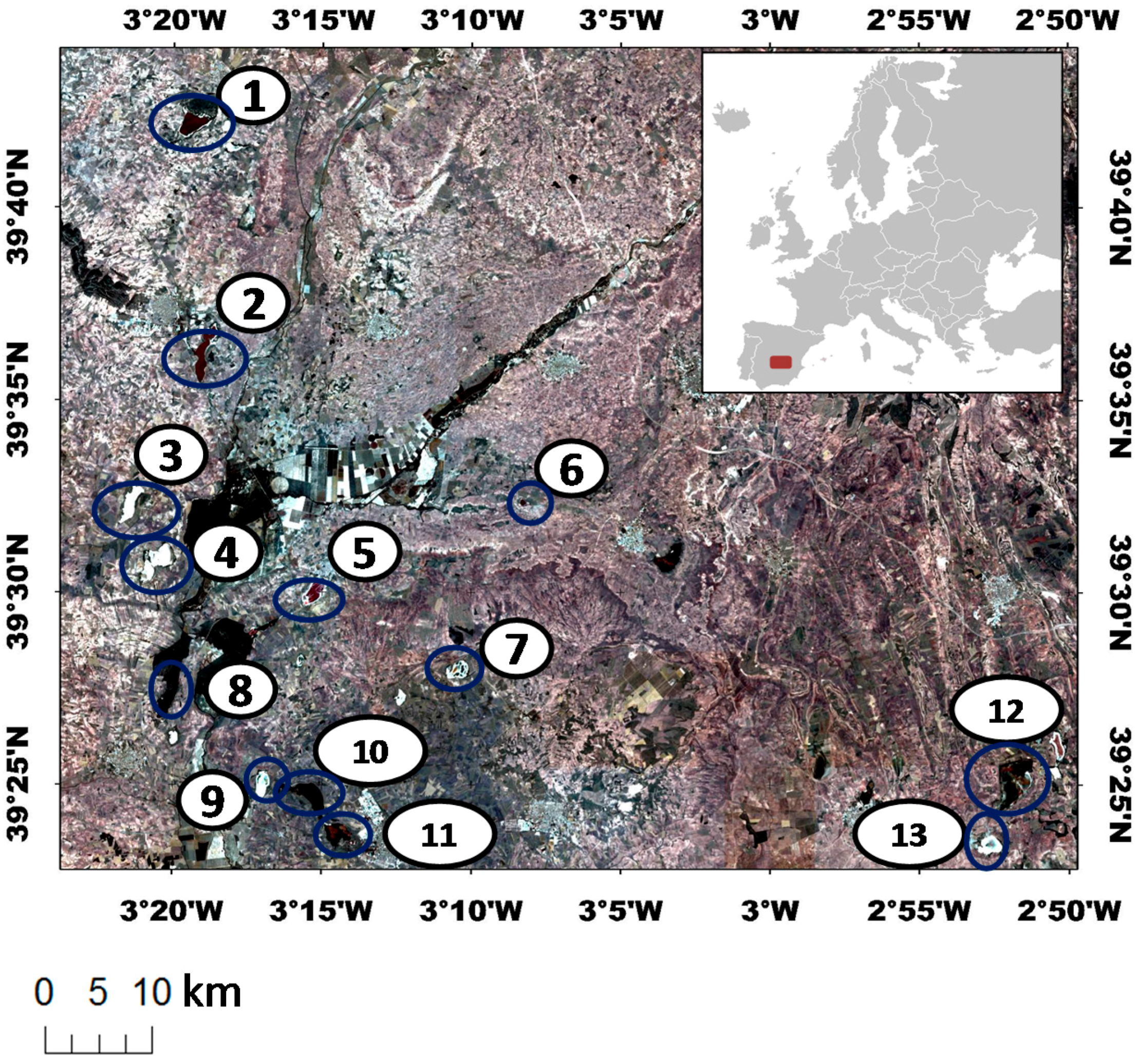
This study is focused on a host of lakes located in the Biosphere Reserve of La Mancha Húmeda, a wetland-rich region, the largest in the Iberian Peninsula, comprising up to 30,000 ha holding wetlands and lakes [28] distributed within the provinces of Albacete, Ciudad Real, Cuenca, and Toledo, in the Castilla-La Mancha region (Central Spain) (Figure 1). In 1981, UNESCO designated the area as the Biosphere Reserve of La Mancha Húmeda within the Man and Biosphere Programme (MAB), a scientific program to promote improved relationships between people and their environments. In 2014, this Biosphere Reserve was recognized as one of the largest wetland areas in Europe, and many of its wetlands are included in the Natura 2000 Network (European Habitats and Birds Directives) and the Convention on Wetlands of International Importance, called the RAMSAR Convention. Located in a very flat area (La Mancha), the Biosphere Reserve includes floodplain lagoons and, particularly a variety of saline lakes, mostly endorheic, and represents one of the main saline lake districts in Europe.
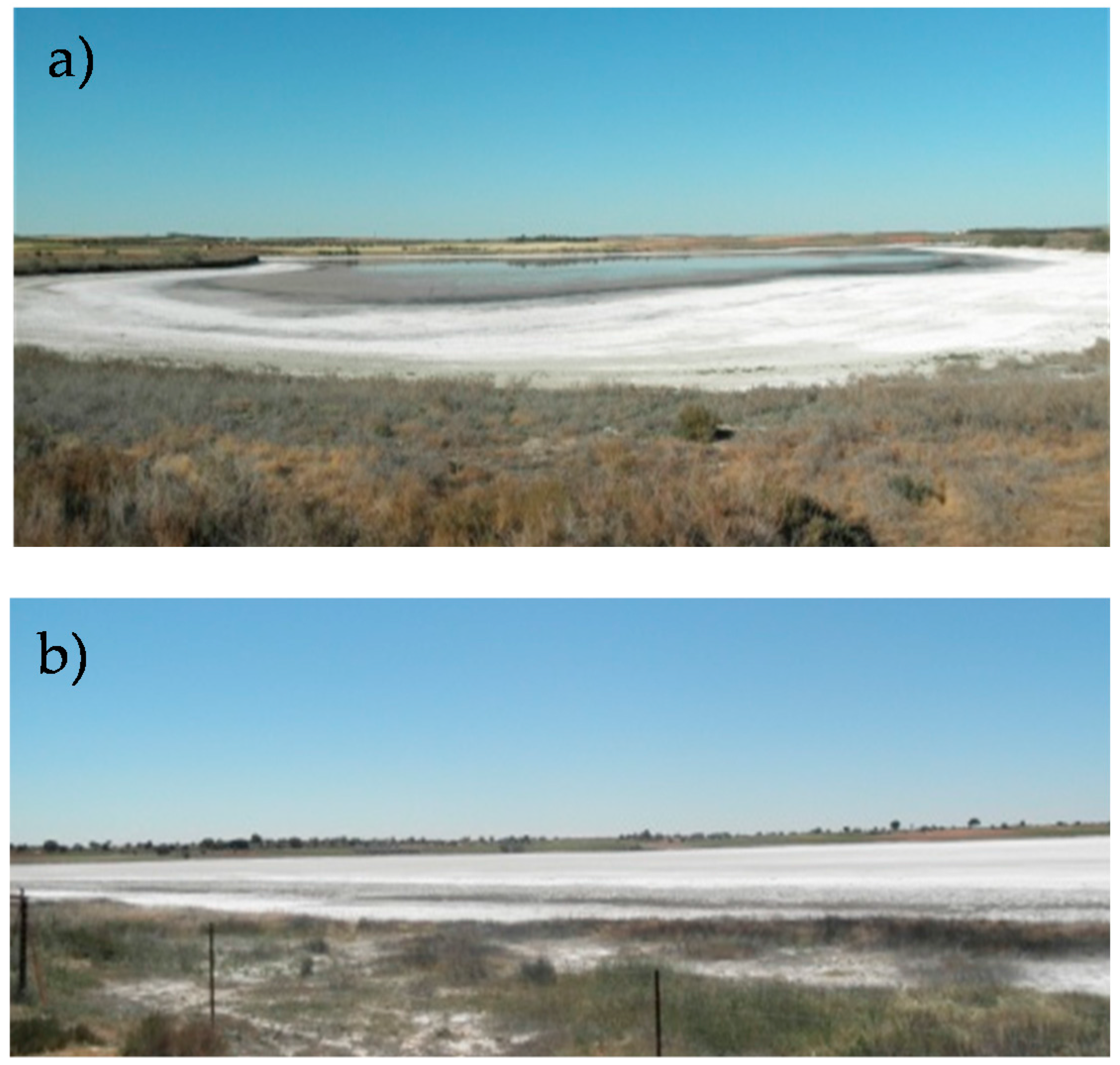
A set of 13 shallow saline lakes were selected for this study (Table 1), all located between 638 and 690 m above sea level. Most are temporary lakes located within the Záncara and Cigüela River Basins in agricultural landscapes. They have small watersheds, mostly covered by vineyards and cereal crops. Most of the lakes have a marginal belt of homophilous plants, and some also have helophytic vegetation in areas where the water is influenced by the discharges of treated wastewater, and thus, salinity is lower in these lakes. The main water inflows to these lakes come from direct precipitation, runoff of small basins, groundwater recharge in some cases and even include some cases of treated wastewater spills from nearby towns. Most of the lakes lack surface outlets and behave as endorheic systems with evaporation as the main water withdrawal process, causing salt accumulation in the lake beds; thus, these lakes range from mesosaline to hypersaline. Their hydroperiods fluctuate, though these lakes are mostly temporary as a result of the mixed Mediterranean-Continental semiarid climate patterns [
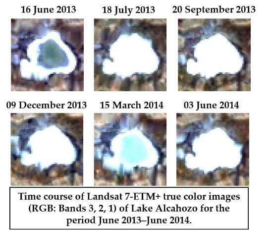
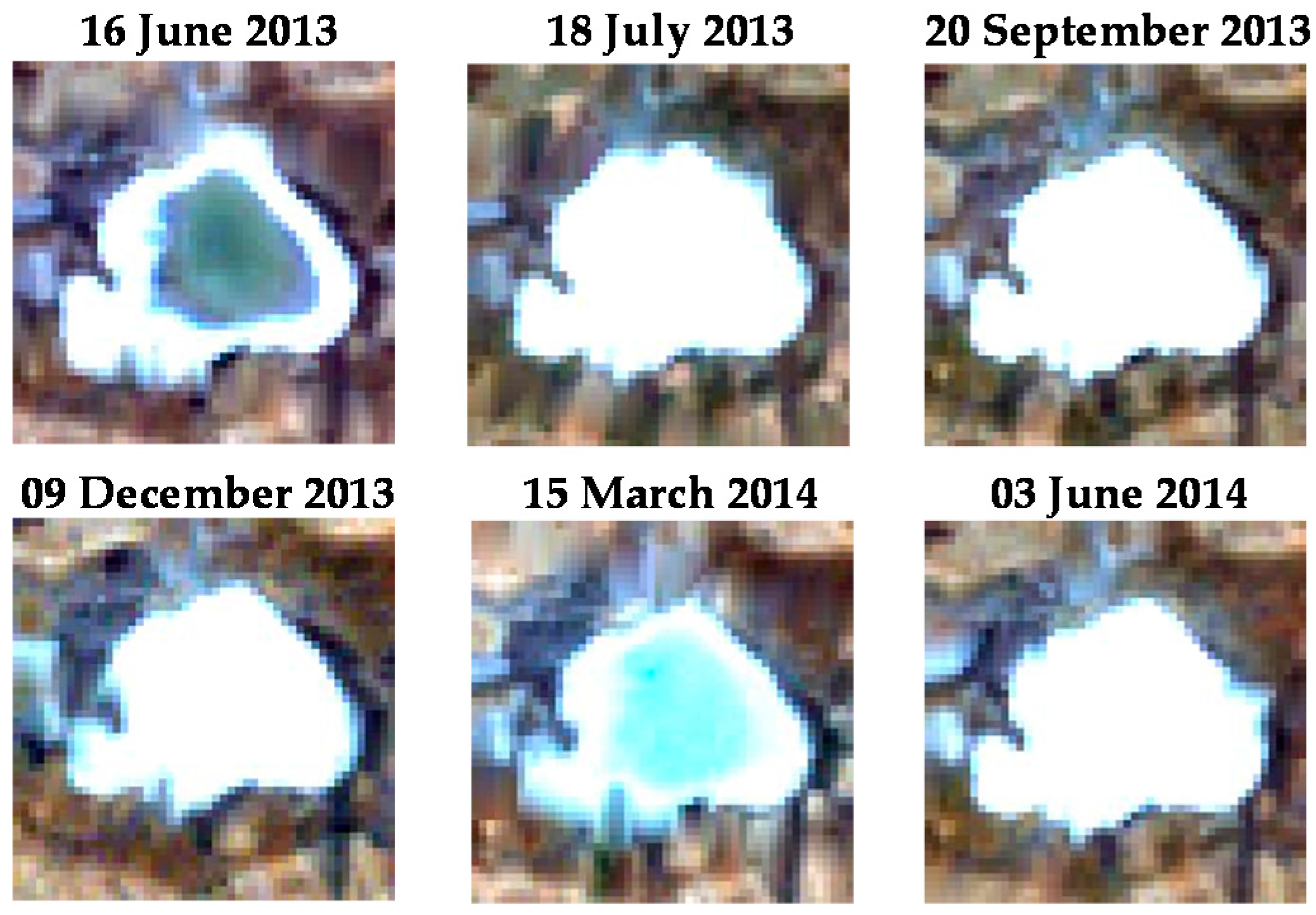
28], which can be illustrated by the flooding pattern of Lake Alcahozo over a specific time horizon (Figure 2). Climate in this area shows a pronounced dry season with average annual rainfall of 400–500 mm [29]. Sediments of the studied area are of continental nature; the terrain is flat; and the dominant lithology is limestone [2].
Lakes in La Mancha Húmeda have rapidly deteriorated because of the alteration of their hydrological patterns and pollution, the former mainly linked to the continuous overexploitation of the aquifers within the last 50 years due to increased agricultural demand [30]. This water extraction caused an unsustainable draft of the aquifers. Many of the lakes within the Biosphere Reserve were drained-out during the 20th century. Others, because of the salinity and the impossibility for agricultural use, were used for landfills or wastewater disposal by the nearby towns.

2.2. Reference Datasets

In addition to the Landsat imagery, three different datasets were used in this study (Table 2): (1) ground-measurements of the water depth in the 13 study lakes, used to test several methods to estimate water pixels coverage and to select the method showing the best performance; (2) the perimeter of two of these lakes (Alcahozo and Manjavacas) measured in situ by GPS; and (3) high spatial resolution Google Earth™ images. The second and third datasets were used to validate the area estimated by the selected method. Boundaries of the lakes obtained from high spatial resolution Google Earth™ images were digitized manually. The water column measurements were collected in the field during 2013–2014 as an integral part of the ECOLAKE project (ecological patterns in plateau lakes: the key for their conservation). Concurrent, or close in time, Landsat overpasses are listed in Table 2. Water depth was monthly measured by limnimeters installed in each lake during the sampling years. A major field campaign was conducted in July 2014 covering lakes Alcahozo, Camino de Villafranca, El Longar, La Veguilla, Las Yeguas and Manjavacas. Satellite images affected by clouds or with an excessive time delay between the acquisition date and field measurements date were discarded.

2.3. Remote Sensing Data Collection and Pre-Processing

The ETM+ onboard Landsat 7 platform was used to conduct this study. All of the images are available free of charge at the United States Geological Survey website. The Landsat cloud-free images downloaded from the EarthExplorer visor (http://earthexplorer.usgs.gov/) correspond to the surface reflectance product corrected from the atmospheric contribution with the 6S radiative transfer code (CDR_sr). The downloaded scenes were synchronous or close in time to the reference data (Table 2). The path and row corresponding to our study area belong to 200/33 and 201/32–33, respectively.
Satellite image pre-processing was required prior the application of the different methods. All scenes were cut to fit our area of interest, and a normalization of the images was then conducted [31,32] using the image of July 2014 as a reference. The iteratively-reweighted multivariate alteration method (IRMAD) was applied [33] to minimize the spectral variability caused by seasonal sun-surface-sensor effects [31]. The IRMAD technique developed for automatic radiometric normalization of multi-spectral and hyper-spectral images allowed us to find linear combinations between the reference and target image bands used to generate a pair of new multispectral images by using canonical correlation analysis. The components of the new images were called canonical variates. This IRMAD technique considers that the reflectance values of some areas in the same scene acquired at different times would be changed, but not everywhere. With this assumption, pixels with the fewest differences between the canonical variates were labeled as the pseudo-invariant pixels, which were then used to normalize each image band-by-band to the reference image. The linear regression equations used to spectrally align each of the six bands of an image were obtained with regression coefficients (r2) > 0.90 and root mean square errors (RMSE) <10%. After this pre-processing, all images were visually compared to ensure that they were co-registered correctly. If so, no further corrections or adjustments were necessary. A correction of the scan line corrector failure was performed following the methodology proposed by Scaramuzza et al. [34]. To isolate our study area (lakes), a water mask was manually digitalized from a Landsat 5-TM image (May 2010), corresponding to a wet year, to mark out the maximum flooding area of the lakes.

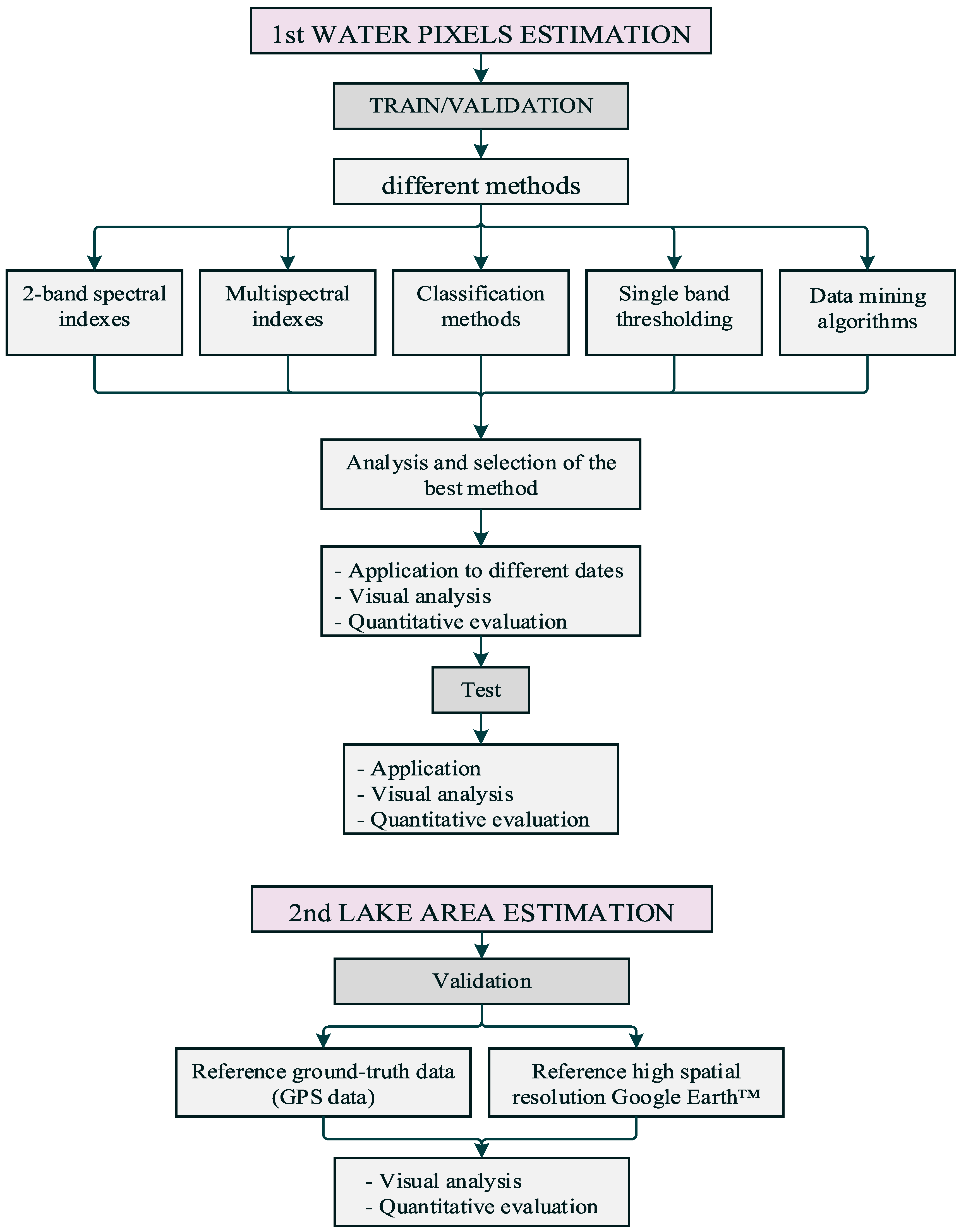
2.4. Water Mapping Methods

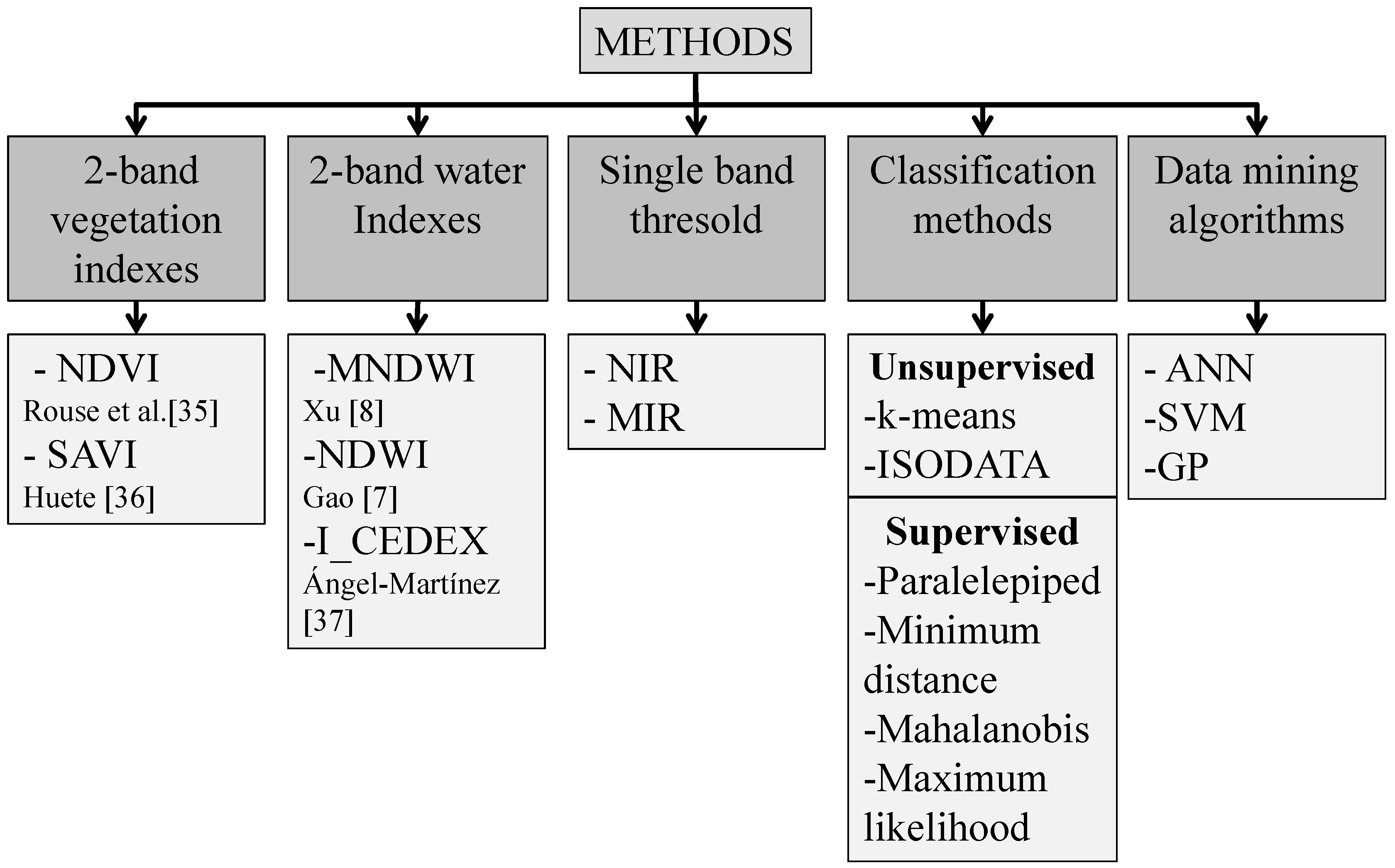
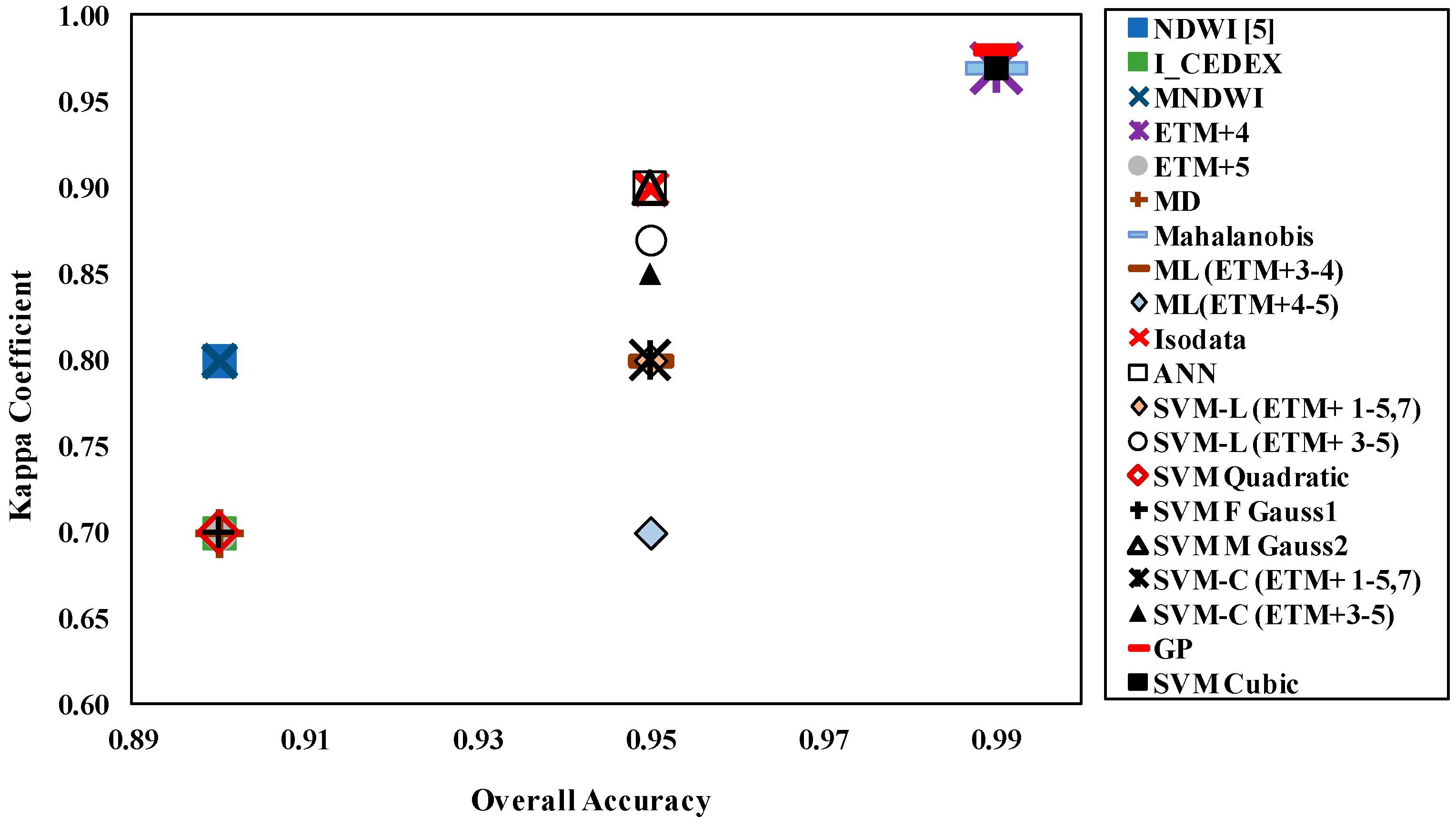
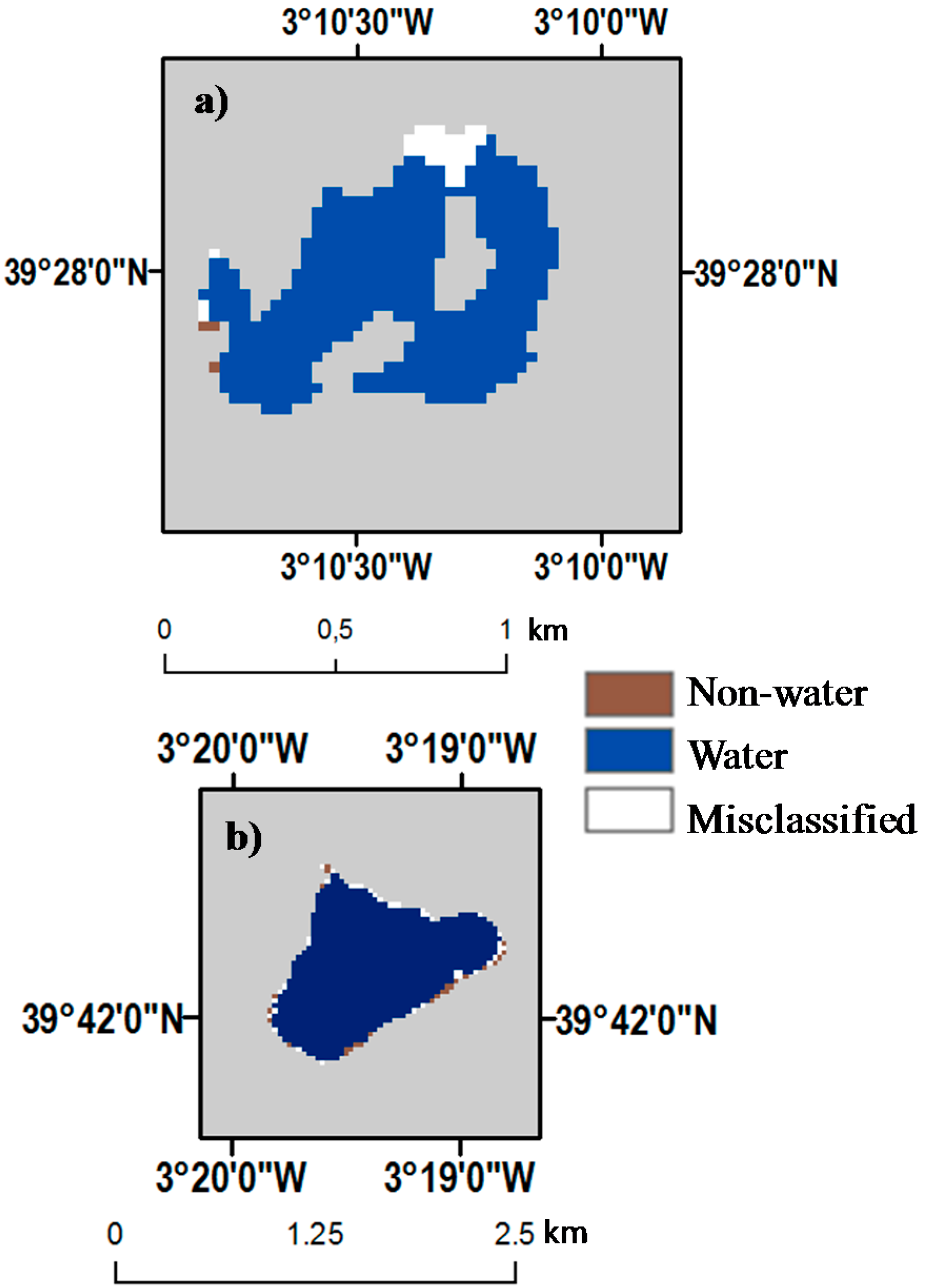
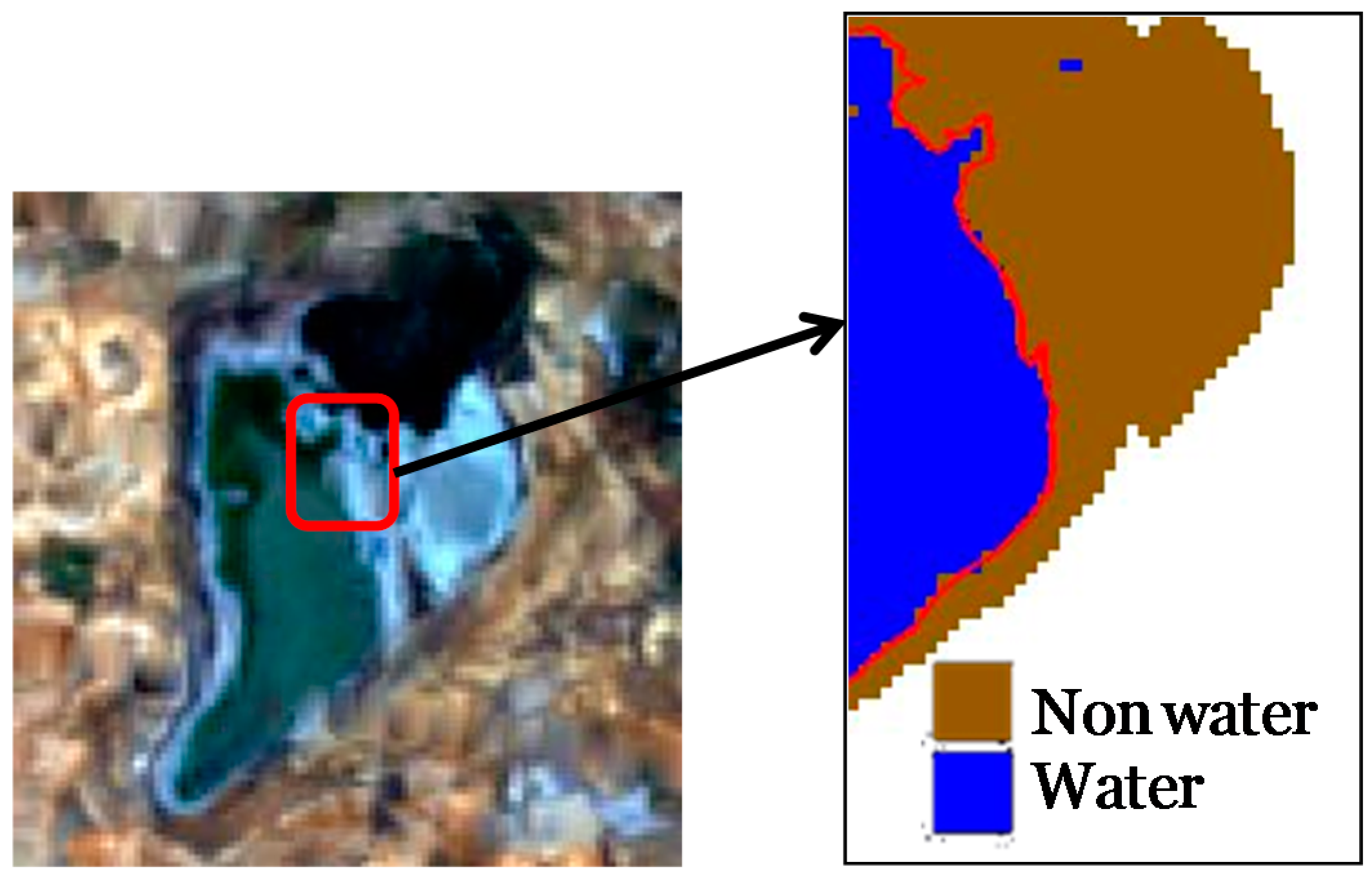
Several methods were tested to estimate the absence or presence of water in the lakebeds of the studied lakes (Figure 3). For a rigorous comparison, we focused on the data from the intensive field campaign in July 2014 and on five tested lakes (Alcahozo, Camino de Villafranca, El Longar, La Veguilla, Las Yeguas and Manjavacas) (Figure 4). The comparison was established between two-band vegetation indices, two-band water indices, single band threshold, classification methods, Artificial Neural Network (ANN), Support Vector Machine (SVM) and Genetic Programming (GP) algorithms. Note that the Landsat image used in this section (21 July 2014) will be later considered as the reference for the normalization procedure applied to the full image dataset. Regarding two-band spectral indices for vegetation, both the NDVI [35] and the SAVI [36] were tested. Within the two-band spectral indices for water, several variants of the NDWI were studied, including the Modification of the Normalized Difference Water Index (MNDWI) and the index proposed by Ángel-Martínez [37] (I_CEDEX) where CEDEX is the Centre for studies and experimentation on public works in Madrid, Spain. The approach proposed by Bustamante et al. [38] based on the MIR band and the single-band threshold with the NIR used by [39] were tested. Both supervised and unsupervised classification methods using different spectral bands were also tested. Unsupervised classification methods include k-means and the Iterative Self-Organizing Data Analysis Technique (ISODATA), whereas supervised classification included the parallelepiped method, minimum and Mahalanobis distance and the maximum likelihood method (Figure 3).
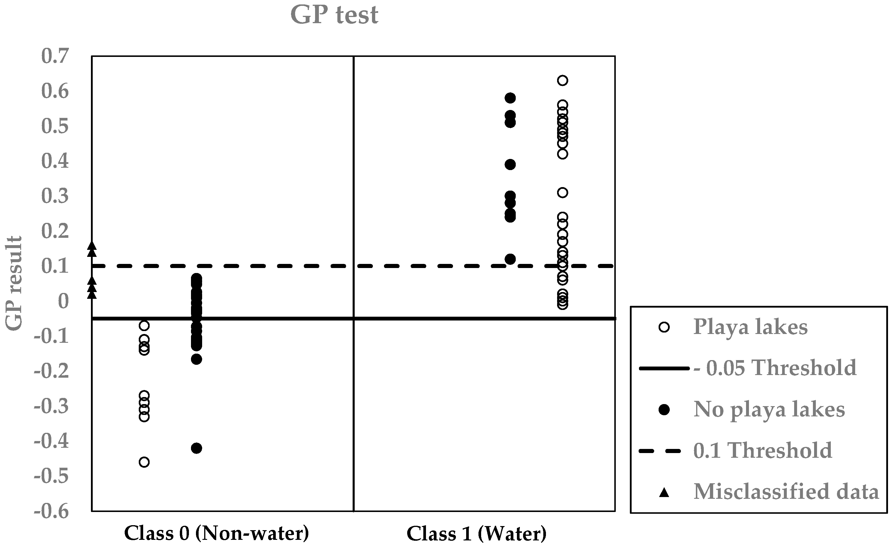
Machine learning algorithms were also considered, including SVM, GP and ANN, a machine-learning method inspired by the human brain function. These machine learning techniques are all nonparametric classification techniques that require no assumptions about the distribution of the data and thus need no a priori knowledge about the characteristics of feature data. An ANN model is based on three different layers: input layer (i.e., input data include reflectance bands and/or water-vegetation indices), one or more hidden layers and the output layer (i.e., dichotomous output includes either water or non-water class) [40]. The SVM is a supervised machine learning technique based on statistical learning theory [41] used to find boundary locations of different classes. In our study, different kinds of SVM were tested to carry out the classification, including linear, quadratic, cubic and Gaussian kernels. MATLAB® software was used to implement ANN and SVM. Finally, genetic programming (GP) is a subclass of evolutionary computation techniques designed to search for the best fit to perform a user-defined task. GP can decode system behaviors based on empirical data for symbolic regression, uncover relationships and make inferences using association path analysis, classification, clustering and forecasting [42]. A principal advantage of GP is that the solution methodology can learn the relationship between the inputs and outputs without any a priori knowledge or preconceptions, thus placing the burden of the discovery process primarily on the GP, reducing data contribution and preprocessing by the user [43]. In this study, the user-defined task was to develop a GP model that uses the inputs of surface reflectance data associated with common bands and different two-band indices to predict the outputs, including water and non-water categories. We used Discipulus® [44] software to run the GP algorithms.
The ground-truth dataset was divided in two subsets for ANN, SVM and GP model training (2/3 of the total data; 56 data points) and validation (1/3 of total data; 28 data points). Finally, the ANN, SVM and GP algorithms yielding the best results were compared to the methods above. A flowchart of the different steps generated in the methodology (Figure 4) shows that all of the pixel values used for the training/validation/testing of all methods were extracted before the correction of the Scan Line Corrector (SLC) failure of Landsat 7; thus, this correction did not cause any bias. A confusion matrix was obtained for each of the methods applied to rank all of the possible cases associated with these models in different categories, estimating whether or not the predicted value is consistent with the real value. To evaluate the consistency of our results, we used the confusion matrix to calculate the kappa coefficient (κ), an index ranging from −1 to +1; values higher than 0.4 are considered acceptable [45]. The confusion matrix can also be used to generate the commission error and user accuracy. The commission error is the percentage of pixels wrongly assigned to a certain class by the classifier, whereas user accuracy is the probability that a pixel assigned to a class by the classifier correctly corresponds to that class. The omission error is the percentage of pixels that belong to the ground truth class, but were improperly classified, and the producer accuracy is the probability that the classifier has been correctly assigned to a class given by the ground truth data.
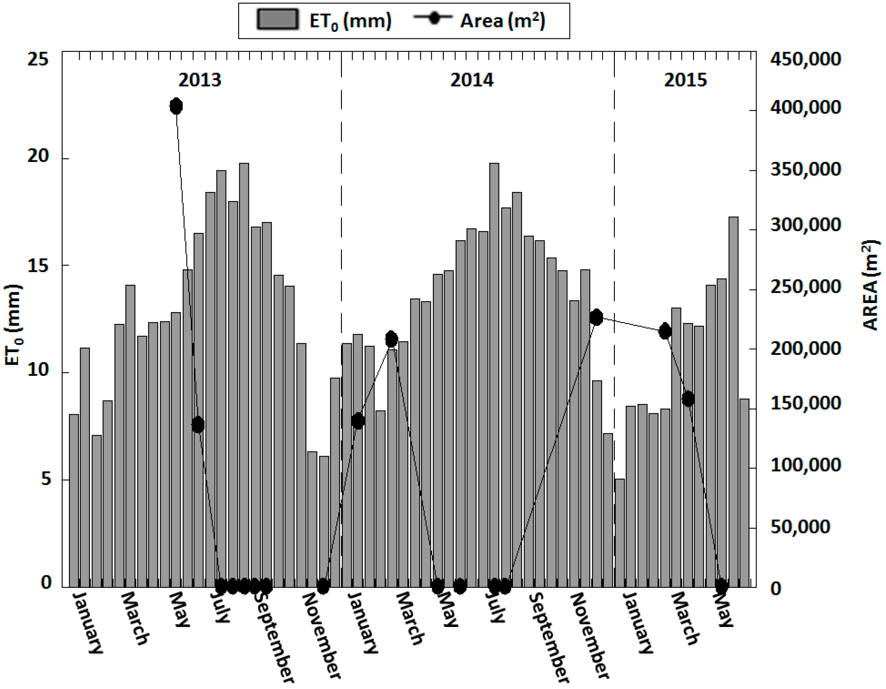
The method showing the best performance in terms of discrimination of water/non-water pixels in our test area was selected and applied to the full set of images listed in Table 2 and to a variety of lakes different from those used in the algorithm training. Finally, the relationship between precipitation- evaporation and the lake water cover was analyzed for Lake Alcahozo, used as a model lake to explore the effect of meteorological variability characteristic of the Mediterranean climate during 2013–2015. Meteorological data were downloaded from the Servicio Integral de Asesoramiento al Regante de Castilla-La Mancha (SIAR) (http://crea.uclm.es/siar/datmeteo/), which provides daily information of mean, absolute maximum and minimum values of temperature, humidity, wind speed, cumulative global solar radiation, daylight hours, precipitation and reference evapotranspiration estimated with the Penman–Monteith equation [46]. In the present study, we focused on precipitation and reference evapotranspiration data to explore the hydrological cycle dynamics.
Finally, we include a brief discussion of climate elasticity as an application example. Climate elasticity of streamflow (e), an index commonly used to quantify the sensitivity of streamflow to meteorological pattern and climate change. It is defined as the proportional change in the streamflow (lake flooded area in our case) relative to the proportional change in a climatic variable, such as precipitation (p). The index was applied to our lake data, and the nonparametric estimator was used to calculate the climate elasticity [47]. In particular, we focused on the variation between the area of a lake and the precipitation Equation (1).
e p = m e d i a n ( A t A ¯ P t P ¯ × P ¯ A ¯ )
where ep is the climate elasticity relative to precipitation, A and P represent area and precipitation, A ¯ and P ¯ are the corresponding yearly mean values and t is time.

3. Results and Discussion

3.1. Water Pixel Estimation

Results of the accuracy assessment of the different methods are summarized in Table 3, Table 4 and Table 5. Among the water indices, the NDWI based on the green and NIR bands [6] (Table 3) showed the best performance. This index showed the best results with the threshold proposed by the original author for to assign water pixels (values > 0). An overall accuracy of 90% and a kappa coefficient of 0.80 were obtained. In the case of the MNDWI and the NDWI [7], the best results were obtained with a threshold of 0.5 and −2 for the I_CEDEX (Table 3).
Kappa values of 0.4 were obtained for the methods based on vegetation indices (NDVI and SAVI) (Table 3). Visualization analysis based on field conditions showed that both water and vegetation indices overestimated the water pixels when the lakes were completely dry in July 2014.
Acceptable results were obtained for the single-band threshold, with kappa values of 0.97 and 0.70 for Bands 4 and 5 (Figure 5), although Band 5 overestimated the water pixels, possibly due to the presence of puddles or mud puddle areas on the lakes surfaces. The water index using near and middle infrared ETM+ bands (NDWI [7]) presented worse results than the other water indexes applied to our study area, possibly because these wavelengths are more sensitive to the presence water [38], thus causing mistakes in the water-cover pixel identification. These results agree with the conclusions of Campos et al. [14] reporting that indices using the middle infrared band can have contrasting performances in detecting seasonal and permanent water. The NDWI using near and middle infrared bands was more sensible for detecting the seasonality of the water cover despite significant overestimations. Although the kappa values were acceptable, the commission and omission errors were high, and the total error (percentage of omission and commission) was greater than 30% in all cases, except for ETM+4, where the total error was 4% (Table 3).
The best results for the supervised classification based on the Mahalanobis distance and maximum likelihood methods (Table 4) were obtained for the combination of red and NIR bands, resulting in kappa values of 0.97 and 0.80, respectively. Overall, the classification methods showed acceptable kappa values (Figure 5), but with an underestimation of water pixels in the classification since one of the lakes with water in the ground-data test date (July 2014) was classified as a dry lake. Acceptable results were obtained from the ISODATA unsupervised classification method, with an overall accuracy of 95% and a kappa value of 0.90. A total error of 15% was obtained from the ISODATA method.
Data mining methods applied in our study showed overall accuracy values greater than 90% and kappa values higher than 0.70 (Figure 5). Results from the combinations of Bands 3–5 as inputs in both ANN and SVM methods were acceptable (Table 5), as they were in some cases using all bands as inputs. An ANN model with four hidden layers presented the best results, with an overall accuracy of 95% and a kappa value of 0.9. Similar results were obtained when applying the SVM with all reflectance bands as inputs. The best results were obtained from the SVM method when using the linear and cubic kernel. In particular, the cubic kernel-based SVM showed the best results with an overall accuracy of 99% and a kappa value close to one.
In contrast to the ANN and SVM methods, the GP algorithm produces a complex relationship between the inputs and outputs via a nonlinear function. The best results were obtained by a relationship between the water pixels and the reflectance of the NIR band from the Landsat ETM+ imagery. The resulting nonlinear equation was:
GPRw = cos ((0.003 × ETM + 4)1/4)
where GPRw is the GP outputs for water classification.
This GP algorithm presented a kappa value of 0.98 and an error of 2% in the classification of the water pixels (Table 5). With such a relationship between the reflectance values and the class given by Equation (2), a threshold could be established to determine whether there is water-cover or not in each pixel. In this study, values of GPRw higher than 0.1 imply that the classification as water pixels is favored.
Based on its accuracy assessment compared to other methods, the GP algorithm was selected as the most appropriate method (Table 5). As explained in the Methods section (Figure 4), this, as the best method, was selected to be applied to a set of images from different dates. First, it was applied for the same lakes for which the algorithm was performed and then applied to the rest of the lakes. When the results of the GP algorithm were applied to the full image dataset (Table 2), an overall accuracy of 95% with a kappa value of 0.8 was achieved. When applied to lakes different from those used in the algorithm training, an overall accuracy of 90% and a kappa value of 0.8 were obtained. We could further discern between two different thresholds to separate water and non-water pixels, one for each type of lake. The lakes in our study area are lakes with wide playas (Figure 6), lakes with smaller playa areas and lakes without playas. Playa lakes showed a different threshold than those for lakes without playas or with small playa areas (Figure 7). For the small playa area lakes, however, we observed that some have a threshold of −0.05, similar to playa lakes, although most of the playa lakes show a 0.1 threshold value. The result of the GP algorithm after applying the test data can be seen in Figure 7. Lakes without playas presented GPRw values higher than 0.1 for pixels with the presence of water (Class 1) and lower than 0.1 for the dry pixels (Figure 7). Instead, for playa lakes the threshold is −0.05, so lower values presented pixels without water.

3.2. Sub-Pixel Extraction

The selected GP algorithm was applied to the synchronous images (or at least close to the date of the field campaigns) and to the high resolution Google Earth™ images (Table 2). The best results in the classification of water pixels were obtained for lakes Grande de Quero, Larga de Villacañas, Las Yeguas, Manjavacas and Peñahueca with kappa values higher than 0.60 and overall accuracies above 80% (Table 6). We were unable to find close reference data to carry out this part of the study for lakes Grande de Villafranca and Mermejuela.
Lakes Alcahozo, Salicor and Longar presented the lowest kappa values of 0.45, 0.15 and 0.53, respectively. The discrepancies in Lake Alcahozo were probably due to the one-week difference between the image acquisition date and the collection date of the reference data in the field. This lake experiences fast changes in water depth because of its low depth and the absence of regular water inflows, presenting challenges to the classification of these edge pixels. The classification output of the GP algorithm is, however, in agreement with the ground-truth data when the lake was completely dry for the 15 May 2011 campaign (Figure 8).
It is noteworthy that the misclassified area of Lake Salicor is flagged by a kappa value of 0.15 (Figure 8), in part because SLC failure created strips in the original ETM+ images, which affected the observation of the lake. Most of the misclassified data belong to Lakes Salicor and El Longar (Figure 8). On the other hand, the proposed GP algorithm could not be validated for lakes Grande de Villafranca, Mermejuela and Tírez because no ground data were available, and the auxiliary Google Earth™ images were distant in time. However, the application of the GP algorithm to a Landsat image of the Lake Manjavacas obtained on 21 May 2015, against the GPS ground measurements of the water perimeter on the same date, confirmed that the threshold value of 0.1 is applicable (Figure 9). In this case, an overall accuracy of 95% and a kappa value of 0.90 were obtained.

3.3. Water Area Variation

The selected GP algorithm was applied to the available images to estimate the flooded area of all studied lakes from spring 2013 to spring 2015. Focusing on Lake Alcahozo, we further present a linkage between climate (precipitation and reference evapotranspiration (ET0)) and the flooded area of the lake to elucidate the link between meteorology and lake hydrology at the local scale. The reference evapotranspiration (ET0) was used as an indicator of the behavior and intensity of the evaporation in our study area. The results of the flooded area estimation for Lake Alcahozo, which is completely dry in summer periods following the seasonal trend typical for this type of lake, are shown in Figure 10. Figure 11 shows that the flooded area was mainly driven by the precipitation pattern, and larger flooded areas were obtained for wetter years. In May 2013, the flooded area presented a maximum value, because lake water remaining from winter was further increased by the March rainfall peak. In addition, this lake presents a dry season in summer, corresponding to the highest ET0 values (Figure 10).
The proportional change in the flooded area with the precipitation was calculated for our study time frame for lakes that presented the best estimations of flooded area. After calculating the climate elasticity, two different values were obtained, around 0.2 and 1.3, in association with a low or high temporality, respectively. All lakes with a strong seasonal trend, such as Lakes Alcahozo, Camino de Villafranca, Grande de Quero and Las Yeguas, presented values of 1.3, indicating that in these two years, a 1% change in mean annual rainfall resulted in a 1.3% change in the mean annual flooded area of these lakes, whereas in the other cases (Lakes Larga de Villacañas, La Veguilla and Manjavacas), a similar change in annual rainfall only resulted in a variation of 0.2% of the mean annual flooded area. This finding is a consequence of the hydrological alteration driven by the wastewater disposal in the second set of lakes, which expanded the flooding period and buffered rainfall-dependent fluctuations in water level.
Although the algorithm was tested for different lakes from our study area and the seasonal effects were minimized with the radiometric normalization, the chemical and biophysical changes in the water bodies could affect the results of the GP algorithm. We tried to minimize these factors by applying the GP algorithm to different seasons and different water levels of each lake. Although the GP algorithm showed acceptable results, the robustness of the described methodology will need to be further assessed using additional datasets. In addition, the SLC failure of Landsat 7 imageries caused errors in the estimation of the total water area of some lakes. Water bodies presenting irregular shapes could be more vulnerable to this issue, such as the case of Salicor Lake in the present study.
The proposed GP algorithm can also be applied to images obtained from other sensors, such as Landsat 5, which will allow us to conduct long-term studies. Future works will deal with the applications to other sensors, such as SPOT-5 or the recent Sentinel 2. The future NASA satellite “Surface Water and Ocean Topographic (SWOT)”, which is expected to be launched in 2020 for a demonstration mission with an expected length of three years, is a good example of the importance of these types of studies. In addition, future prospects of our current work will be the long-term monitoring of the lakes to study their hydrological patterns in greater detail to help to develop adequate management plans for lake protection, conservation and recovery under the European Water Framework and the Habitats Directives, especially for semiarid regions, such as the Mediterranean basin.

4. Conclusions

Several supervised and unsupervised classification methods to estimate water pixels across a set of 13 shallow saline lakes in Spain were tested and validated in this study, using Landsat 7-ETM+ imageries. These methods tested include the two-band spectral indices, multispectral indices, classification methods, single threshold and the data mining or machine learning techniques. The GP algorithm showed the best performance with a kappa value of 0.98 and a low error of 2%, both in training and validation. The robustness of this GP method was reinforced with additional ground-truth data. This GP algorithm could serve as a tool to improve our understanding of the temporal trends in seasonal lakes and their dependence on meteorological patterns, especially on rainfall. Such an approach provides a cost-effective way to monitor the flooded area variations related to changes of precipitation and evaporation, as well as to resource exploitation, in order to establish sustainable water resources management plans that preserve the ecological health of wetlands and lakes in semiarid basins with a high water stress, such as the area of La Mancha Húmeda Biosphere Reserve.

Acknowledgments

This study was jointly supported by the Spanish Ministry of Economy and Competitiveness and the European Regional Development Fund (FEDER) "One way to make Europe”, through the projects: “CLIMAWET” CGL2015-69557-R (MINECO/FEDER,UE), “ECOLAKE” (CGL2012-38909) and “ESCLITEL” (CGL2013-46862-C2-1/2-P), the first two to A.C., by the Regional Government of Valencia through the project PROMETEOII/2014/086 and postdoctoral contract of V. García-Santos (“VALi+D” APOSTD /2015/033). The authors would like to thank García-Haro and S. Sánchez-Ruíz for their comments. Finally, the authors want to thank the valuable and detailed reviewers’ comments.

Author Contributions

C.D., N.-B.C. and A. C. conceived and designed the experiments; C.D. performed the experiments; C.D., N.-B.C. and A.C analyzed the data; V.C., J.M.S., L.P.-P., V.G.-S., M.M.B. and S.I. contributed reagents/materials/analysis tools and field campaigns. C.D., N-B.C., J.M.S. and A. C. wrote the paper.

Conflicts of Interest

The authors declare no conflict of interest.

References

  1. Florín, M.; Montes, C.; Rueda, F. Origin, hydrologic functioning, and morphometric characteristics of small, shallow, semiarid lakes (lagunas) in La Mancha, central Spain. Wetlands 1993, 13, 247–259. [Google Scholar] [CrossRef]
  2. Gosálvez, R.; Gil-Delgado, J.A.; Vives-Ferrándiz, C.; Sánchez, G.; Florín, M. Seguimiento de aves acúaticas amenazadas en lagunas dela Reserva de la Biosfera de La Mancha Húmeda (España central). Polígonos 2012, 22, 89–122. [Google Scholar] [CrossRef]
  3. Castañeda, C.; Herrero, J. Teledeección de cambios en la Laguna de Gallocanta. Memorias Real Soc. Española Hist. Nat. 2009, 7, 103–126. [Google Scholar]
  4. Camacho, A.; Miracle, M.R.; Vicente, E. Which factors determine the abundance and distribution of picocyanobacteria in inland waters? A comparison among different types of lakes and ponds. Arch. Hydrobiol. 2003, 157, 321–338. [Google Scholar] [CrossRef]
  5. Work, E.A.; Gilmer, D.S. Utilization of satellite data for inventorying prairie ponds and lakes. J. Photogramm. Eng. Remote Sens. 1976, 42, 685–694. [Google Scholar]
  6. McFeeters, S.K. The use of the Normalized Difference Water Index (NDWI) in the delineation of open water features. Int. J. Remote Sens. 1996, 17, 1425–1432. [Google Scholar] [CrossRef]
  7. Gao, B.C. NDWI—A normalized difference water index for remote sensing of vegetation liquid water from space. Remote Sens. Environ. 1996, 58, 257–266. [Google Scholar] [CrossRef]
  8. Xu, H. Modification of normalised difference water index (NDWI) to enhance open water features in remotely sensed imagery. Int. J. Remote Sens. 2006, 27, 3025–3033. [Google Scholar] [CrossRef]
  9. Bai, J.; Chen, X.; Li, J.; Yang, L.; Fang, H. Changes in the area of inland lakes in arid regions of central Asia during the past 30 years. Environ. Monit. Assess. 2011, 178, 247–256. [Google Scholar] [CrossRef] [PubMed]
  10. McFeeters, S.K. Using the normalized difference water index (NDWI) within a geographic information system to detect swimming pools for mosquito abatement: A practical approach. Remote Sens. 2013, 5, 3544–3561. [Google Scholar] [CrossRef]
  11. Sakamoto, T.; Van Nguyen, N.; Kotera, A.; Ohno, H.; Ishitsuka, N.; Yokozawa, M. Detecting temporal changes in the extent of annual flooding within the Cambodia and the Vietnamese Mekong Delta from MODIS time-series imagery. Remote Sens. Environ. 2007, 109, 295–313. [Google Scholar] [CrossRef]
  12. Li, W.; Du, Z.; Ling, F.; Zhou, D.; Wang, H.; Gui, Y.; Sun, B.; Zhang, X. A comparison of land surface water mapping using the normalized difference water index from TM, ETM+ and ALI. Remote Sens. 2013, 5, 5530–5549. [Google Scholar] [CrossRef]
  13. El-Asmar, H.M.; Hereher, M.E. Change detection of the coastal zone east of the Nile Delta using remote sensing. Environ. Earth Sci. 2011, 62, 769–777. [Google Scholar] [CrossRef]
  14. Campos, J.C.; Sillero, N.; Brito, J.C. Normalized difference water indexes have dissimilar performances in detecting seasonal and permanent water in the Sahara-Sahel transition zone. J. Hydrol. 2012, 464-465, 438–446. [Google Scholar] [CrossRef]
  15. Maglione, P. Coastline extraction using high resolution WorldView-2 satellite imagery. Eur. J. Remote Sens. 2014, 685–699. [Google Scholar] [CrossRef]
  16. Ji, L.; Zhang, L.; Wylie, B. Analysis of dynamic thresholds for the normalized difference water index. Photogramm. Eng. Remote Sens. 2009, 75, 1307–1317. [Google Scholar] [CrossRef]
  17. Jain, S.K.; Singh, R.D.; Jain, M.K.; Lohani, A.K. Delineation of flood-prone areas using remote sensing techniques. Water Resour. Manag. 2005, 19, 333–347. [Google Scholar] [CrossRef]
  18. Ouma, Y.O.; Tateishi, R. A water index for rapid mapping of shoreline changes of five East African Rift Valley lakes: An empirical analysis using Landsat TM and ETM+ data. Int. J. Remote Sens. 2006, 27, 3153–3181. [Google Scholar] [CrossRef]
  19. Lira, J. Segmentation and morphology of open water bodies from multispectral images. Int. J. Remote Sens. 2006, 27, 4015–4038. [Google Scholar] [CrossRef]
  20. Fisher, A.; Danaher, T. A water index for SPOT5 HRG satellite imagery, New South Wales, Australia, determined by linear discriminant analysis. Remote Sens. 2013, 5, 5907–5925. [Google Scholar] [CrossRef]
  21. Gardelle, J.; Hiernaux, P.; Kergoat, L.; Grippa, M. Less rain, more water in ponds: A remote sensing study of the dynamics of surface waters from 1950 to present in pastoral Sahel (Gourma region, Mali). Hydrol. Earth Syst. Sci. Discuss. 2009, 6, 5047–5083. [Google Scholar] [CrossRef]
  22. Soliman, G.; Soussa, H. Wetland change detection in Nile swamps of southern Sudan using multitemporal satellite imagery. J. Appl. Remote Sens. 2011, 5, 053517. [Google Scholar] [CrossRef]
  23. Sun, F.; Sun, W.; Chen, J.; Gong, P. Comparison and improvement of methods for identifying waterbodies in remotely sensed imagery. Int. J. Remote Sens. 2012, 33, 6854–6875. [Google Scholar] [CrossRef]
  24. Feyisa, G.L.; Meilby, H.; Fensholt, R.; Proud, S.R. Automated water extraction index: A new technique for surface water mapping using Landsat imagery. Remote Sens. Environ. 2014, 140, 23–35. [Google Scholar] [CrossRef]
  25. Klein, I.; Dietz, A.J.; Gessner, U.; Galayeva, A.; Myrzakhmetov, A.; Kuenzer, C. Evaluation of seasonal water body extents in Central Asia over the past 27 years derived from medium-resolution remote sensing data. Int. J. Appl. Earth Obs. Geoinf. 2014, 26, 335–349. [Google Scholar] [CrossRef]
  26. Moser, L.; Voigt, S.; Schoepfer, E. Monitoring of critical water and vegetation anomalies of Sub-Saharan West-African wetlands. In Proceedings of the IEEE International Conference on Geoscience and Remote Sensing Symposium, Québec City, QC, Canada, 13–18 July 2014; pp. 3842–3845.
  27. Sethre, P.; Rundquist, B.; Todhunter, P. Remote detection of prairie pothole ponds in the Devils Lake Basin, North Dakota. GISci. Remote Sens. 2005, 42, 277–296. [Google Scholar] [CrossRef]
  28. Laguna, C.; Gosálvez, R.; Sánchez, G.; Falomir, J.; Velasco, A.; Florín, M.; Gil-Delgado, J.; Chicote, A. Climate change footprint in the Mancha húmeda biosphere reserve. In Proceedings of the Energy and Environment Knowledge Week, Toledo, Spain, 28–29 October 2013; pp. 183–185.
  29. Vidal, D.; Anza, I.; Taggart, M.A.; Pérez-ramírez, E.; Crespo, E.; Hofle, U.; Mateo, R. Environmental factors influencing the prevalence of a Clostridium botulinum type C/D mosaic strain in nonpermanent Mediterranean wetlands. Appl. Environ. Microbiol. 2013, 79, 4264–4271. [Google Scholar] [CrossRef] [PubMed]
  30. Florín, M.; Montes, C. Functional analysis and restoration of Mediterranean lagunas in the Mancha Húmeda Biosphere Reserve ( Central Spain). Plant Ecol. 1999, 109, 97–109. [Google Scholar]
  31. Schroeder, T.A.; Wulder, M.A.; Healey, S.P.; Moisen, G.G. Mapping wildfire and clearcut harvest disturbances in boreal forests with Landsat time series data. Remote Sens. Environ. 2011, 115, 1421–1433. [Google Scholar] [CrossRef]
  32. Yang, J.; Weisberg, P.J.; Bristow, N.A. Landsat remote sensing approaches for monitoring long-term tree cover dynamics in semi-arid woodlands: Comparison of vegetation indices and spectral mixture analysis. Remote Sens. Environ. 2012, 119, 62–71. [Google Scholar] [CrossRef]
  33. Canty, M.J.; Nielsen, A.A. Automatic radiometric normalization of multitemporal satellite imagery with the iteratively re-weighted MAD transformation. Remote Sens. Environ. 2008, 112, 1025–1036. [Google Scholar] [CrossRef]
  34. Scaramuzza, P.; Micijevic, E.; Chander, G. SCL Gap-Filled Products. Phase One Methodology; USGS-United States Geology Survey: USA, 2004. Available online: https://landsat.usgs.gov/documents/SLC_Gap_Fill_Methodology.pdf (accessed on 17 September 2014).
  35. Rouse, J.W.; Haas, R.H.; Deering, D.W.; Sehell, J.A. Monitoring the Vernal Advancement and Retrogradation (Green Wave Effect) of Natural Vegetation; Remote Sensing Center. Report RSC 1978-4; Texas A&M University: College Station, TX, USA, 1974. [Google Scholar]
  36. Huete, A.R. A soil-adjusted vegetation index (SAVI). Remote Sens. Environ. 1988, 25, 295–309. [Google Scholar] [CrossRef]
  37. Ángel-Martínez, M.C. Aplicación de la Teledetección en la Localización de Superficies de Agua; CEDEX: Madrid, Spain, 1994. [Google Scholar]
  38. Bustamante, J.; Díaz-Delgado, R.; Aragonés, D.; Pacios, F. Determining water body characteristics of Doñana shallow marshes through remote sensing. In Proceedings of the IEEE International Conference on Geoscience and Remote Sensing Symposium, Denver, CO, USA, 31 July–4 August 2006; pp. 3662–3663.
  39. Doña, C.; Sanchez, J.M.; Caselles, V.; Dominguez, J.A.; Camacho, A. Empirical Relationships for Monitoring Water Quality of Lakes and Reservoirs Through Multispectral Images. IEEE J. Sel. Top. Appl. Earth Obs. Remote Sens. 2014, 7, 1632–1641. [Google Scholar] [CrossRef]
  40. Srivastava, P.K.; Han, D.; Rico-Ramirez, M.A.; Bray, M.; Islam, T. Selection of classification techniques for land use/land cover change investigation. Adv. Sp. Res. 2012, 50, 1250–1265. [Google Scholar] [CrossRef]
  41. Smola, A.J.; Schölkopf, B. A tutorial on support vector regression. Stat. Comput. 2004, 14, 199–222. [Google Scholar] [CrossRef]
  42. Seifert, J.W. Data mining: An overview. In National Security Issues; Pegarkov, D.D., Ed.; Nova Science Publishers, Inc.: New York, NY, USA, 2006; pp. 201–217. [Google Scholar]
  43. Doña, C.; Chang, N.B.; Caselles, V.; Sánchez, J.M.; Camacho, A.; Delegido, J.; Vannah, B.W. Integrated satellite data fusion and mining for monitoring lake water quality status of the Albufera de Valencia in Spain. J. Environ. Manag. 2015, 151, 416–426. [Google Scholar]
  44. Francone, D. Discipulus Software Owner’s Manual, Version 3.0 DRAFT; Machine Learning Technologies, Inc.: Littleton, CO, USA, 1998. [Google Scholar]
  45. Landis, J.R.; Koch, G.G. The measurement of observer agreement for categorical data. Biometrics 1977, 33, 159–174. [Google Scholar] [CrossRef] [PubMed]
  46. Allen, R.G.; Pereira, L.S.; Raes, D.; Smith, M.; Ab, W. Crop Evapotranspiration—Guidelines for Computing Crop Water Requirements—FAO Irrigation and Drainage Paper 56; FAO: Rome, Italy, 1998; pp. 1–15. [Google Scholar]
  47. Sankarasubramanian, A.; Vogel, R.M.; Limbrunner, J.F. Climate elasticity of stream ow in the United States. Water Resour. 2001, 37, 1771–1781. [Google Scholar] [CrossRef]
Figure 1. Landsat 5 true color image (RGB: 3, 2 and 1) of the study area. The studied lakes are: (1) El Longar; (2) Larga de Villacañas; (3) Tírez; (4) Peñahueca; (5) Grande de Quero; (6) Mermejuela; (7) Salicor; (8) Grande de Villafranca; (9) Las Yeguas; (10) Camino de Villafranca; (11) La Veguilla; (12) Manjavacas; and (13) Alcahozo.
Remotesensing 08 00618 g001
Figure 2. Time course of Landsat 7-ETM+ true color images (RGB: Bands 3, 2, 1) of Lake Alcahozo for the period June 2013–June 2014.
Remotesensing 08 00618 g002
Figure 3. Collection of methods to estimate water pixels tested in this work. ISODATA, Iterative Self-Organizing Data Analysis Technique.
Remotesensing 08 00618 g003
Figure 4. Flow chart showing the different steps followed in the methodology to determine the most appropriate water estimation method. (Lake abbreviations: Alcahozo, AL; Camino de Villafranca, CA; Grande de Quero, QUE; Grande de Villafranca, GRAN; La Veguilla, VE; Larga de Villacañas, LAR; Las Yeguas, YE; Longar, LO; Manjavacas, MAN; Mermejuela, MER Peñahueca, PE; Salicor, SAL; Tírez, TI).
Remotesensing 08 00618 g004
Figure 5. Kappa coefficient vs. overall accuracy for the methods showing acceptable kappa values: water-vegetation indices and single bands, classification and data mining methods.
Remotesensing 08 00618 g005
Figure 6. Playa lakes: (a) Camino de Villafranca and (b) Alcahozo.
Remotesensing 08 00618 g006
Figure 7. Different thresholds obtained after applying the GP algorithm to the test data. Class 0 belongs to dry pixels and Class 1 to water pixels. Data for playa lakes (white circles) are differentiated from those of lakes having small or no playas (black circles).
Remotesensing 08 00618 g007
Figure 8. Results of the classification from the GP algorithm for (a) Salicor and (b) El Longar for the reference date 9 February 2011 and Landsat image of 3 February 2011.
Remotesensing 08 00618 g008
Figure 9. Results of the classification using the GP algorithm for Lake Manjavacas for 21 May 2015 (0.1 threshold). The red line represents the GPS track of the water limit, measured in situ.
Remotesensing 08 00618 g009
Figure 10. The flooded area in relation to reference evapotranspiration (ET0) for the period 2013–2015 in Lake Alcahozo.
Remotesensing 08 00618 g010
Figure 11. The flooded area in relation to precipitation for the period 2013–2015 in Lake Alcahozo.
Remotesensing 08 00618 g011
Table 1. Main features of the study lakes.
Lake *1Coordinates °NCoordinates °WAltitude (masl)Max Area *2 (km2)Seasonality
Alcahozo (13)39.382.856600.19High
Camino de Villafranca (10)39.413.266381.4Moderate
Grande de Quero (5)39.503.246640.9High
Grande de Villafranca (8)39.463.336450.9Low
La Veguilla (11)39.393.246380.19Low+
Larga de Villacañas (2)39.623.346601.4Low+
Las Yeguas (9)39.413.286380.6High
El Longar (1)39.703.326900.3High
Manjavacas (12)39.412.866701.4Moderate+
Mermejuela (6)39.543.136600.09High
Peñahueca (4)39.513.346501.6High
Salicor (7)39.473.176680.6High
Tírez (3)39.543.366501.3High
*1 In brackets, the lake identification number (from Figure 1); *2 source: Guadiana River Basin Administration (http://www.chguadiana.es/); +, these lakes receive treated wastewater inputs that artificially increase the water supply.
Table 2. Data sources for this study for each lake: A = ground-measurements of the water depth, B = GPS data and C = Earth Explorer™ ©Digital globe, respectively (lake abbreviations as follows: Alcahozo, AL; Camino de Villafranca, CA; Grande de Quero, QUE; Grande de Villafranca, GRAN; La Veguilla, VE; Larga de Villacañas, LAR; Las Yeguas, YE; Longar, LO; Manjavacas, MAN; Mermejuela, MER Peñahueca, PE; Salicor, SAL; Tírez, TI).
Landsat Image Date (Day/Month/Year)Reference Data Date (Day/Month/Year)SourceLakes
3 February 20119 February 2011CLO/YE/CA/VE/LAR/PE/QUE/SAL
29 June 201229 June 2012CVE/LAR/PE
7 July 201215 July 2012CCA/SAL
24 February 201328 February 2013AAL/CA/MAN
31 May 201329 May 2013AAL/CA/LO/VE/MAN/GRAN/LAR/MER/PE/QUE/TI
25 July 201323 July 2013ACA/VE/YE/QUE/TI
29 October 201328 October 2013APE/TI
23 November 201325 November 2013AAL/CA/LO/LAR/SAL
16 December 201316 December 2013ACA/LO/GRAN/LAR/PE/TI
26 January 201427 January 2014ACA/VE/MAN/YE/PE/TI
5 February 201429 April 2014ACA/MER
26 June 201424 June 2014ALO/VE/YE/GRAN/LAR/MER/QUE/SAL
21 July 201423 July 2014 *AAL/CA/LO/VE/MAN/YE/MER/PE/TI
2 March 201522 February 2015BAL/MAN
21 May 201521 May 2015BAL/MAN
* Field inspection work in AL/CA/LO/VE/MAN/YE.
Table 3. Summary of accuracy assessment of the different water and vegetation indices and the single bands tested.
Method Overall Accuracy (%)KappaCommission Error (%)Omission Error (%)Producer Accuracy (%)User Accuracy (%)Total Error (%)
MNDWIXu [8]900.80303957030
NDWIGao [7]900.604015856060
NDWIMcFeeters [6]900.80253957530
I_CEDEXÁngel-Martínez [37]900.704010906050
NDVIRouse et al. [35]700.406030704090
SAVIHuete [36]700.406030704090
ETM+4 990.972298984
ETM+5 900.704001006040
Table 4. Summary of the accuracy assessment for the different classification methods and band combinations tested in this study.
Method Overall Accuracy (%)KappaCommission Error (%)Omission Error (%)Producer Accuracy (%)User Accuracy (%)Total Error (%)
ParallelepipedAll combinations<40<0.20>50>50<50<50>60
Minimum distanceETM+ 4,5900.674001006060
MahalanobisETM+ 3,4990.9750100955
Maximum LikelihoodETM+ 3,4950.800307010030
Maximum LikelihoodETM+ 4,5950.700406010040
K-meansETM+ 4,5800.601030907540
K-meansETM+ 4800.601030907540
ISODATAETM+ 3,4950.901051008015
Table 5. Summary of the accuracy assessment of the different data mining methods tested.
Method Overall Accuracy (%)KappaCommission Error (%)Omission Error (%)Producer Accuracy (%)User Accuracy (%)Total Error (%)
ANNETM+ 1–5,7950.90415859519
SVM linearETM+ 1–5,7950.800151008515
SVM linearETM+ 3–5950.870181008018
SVM QuadraticETM+ 3–5900.700401006540
SVM CubicETM+ 1–5,7990.9706100946
SVM F Gauss1ETM+ 3–5900.700401005940
SVM M Gauss2ETM+ 3–5950.900201008020
SVM CourseETM+ 1–5,7950.800301007530
SVM CourseETM+ 3–5950.850201007920
GPETM+ 4990.9820100972
Table 6. Accuracy in the estimation of water area for the different lakes with reference data.
Lake *1ThresholdOverall Accuracy (%)Kappa
Alcahozo (13)−0.05700.45
Camino de Villafranca (10)−0.05940.62
Grande de Quero (5)−0.05990.85
* La Veguilla (11)0.10860.68
Larga de Villacañas (2)0.10900.61
* Larga de Villacañas (2)0.10800.80
Las Yeguas (9)−0.05970.76
El Longar (1)−0.05960.53
Manjavacas (12)0.10960.92
Manjavacas (12)0.10860.73
* Peñahueca (4)−0.05950.82
Salicor (7)−0.05940.15
* Synchronous reference and satellite data (same day); *1 lake identification number listed in each bracket as in Figure 1.

