
Forecasting the Crude Oil Spot Price with Bayesian Symbolic Regression
Faculty of Economic Sciences, University of Warsaw, 00-927 Warsaw, Poland
Energies 2023, 16(1), 4; https://doi.org/10.3390/en16010004
Submission received: 17 November 2022
/
Revised: 28 November 2022
/
Accepted: 29 November 2022
/
Published: 20 December 2022
Abstract
:In this study, the crude oil spot price is forecast using Bayesian symbolic regression (BSR). In particular, the initial parameters specification of BSR is analysed. Contrary to the conventional approach to symbolic regression, which is based on genetic programming methods, BSR applies Bayesian algorithms to evolve the set of expressions (functions). This econometric method is able to deal with variable uncertainty (feature selection) issues in oil price forecasting. Secondly, this research seems to be the first application of BSR to oil price forecasting. Monthly data between January 1986 and April 2021 are analysed. As well as BSR, several other methods (also able to deal with variable uncertainty) are used as benchmark models, such as LASSO and ridge regressions, dynamic model averaging, and Bayesian model averaging. The more common ARIMA and naïve methods are also used, together with several time-varying parameter regressions. As a result, this research not only presents a novel and original application of the BSR method but also provides a concise and uniform comparison of the application of several popular forecasting methods for the crude oil spot price. Robustness checks are also performed to strengthen the obtained conclusions. It is found that the suitable selection of functions and operators for BSR initialization is an important, but not trivial, task. Unfortunately, BSR does not result in forecasts that are statistically significantly more accurate than the benchmark models. However, BSR is computationally faster than the genetic programming-based symbolic regression.
1. Introduction
There are numerous studies showing that during different time periods, different sets of explanatory variables might play a major role as oil price predictors. For example, during the period before the 1980s, much attention was focused solely on supply and demand factors. However, it was observed that during the 1990s, the role of exchange rates became crucial. Moreover, since the 2000s, much attention has turned towards several other factors, mostly from financial markets, such as stock market indices, stress market indices, global economic activity, etc. [1,2,3]. Some researchers have focused on tight and complicated links between futures and spot prices. Interestingly, several of them have noticed that, for example, fluctuations in open interest (i.e., the total number of not-closed or not-delivered options or futures) can serve as a better proxy for the futures market than just futures prices [4]. Moreover, several other factors and indices have been considered, such as those connected with policy uncertainty. [5,6,7]. As a result, forecasting methods allowing for the state–space of the model to vary in time have gained much attention [2,3,8,9,10]. Detailed analyses and reviews of how these variables can play an important role as crude oil spot price predictors have been presented in numerous other papers or in review articles solely devoted to this problem [2,11,12,13,14].
Motivation for the current research arises from the fact that symbolic regression has not yet been extensively applied in economics or finance. Even if certain studies have been conducted in the field of oil markets, they have been mostly focused on forecasting production or emission quotas—not on spot price forecasting in the presence of variable (and model) uncertainty [15,16]. On the contrary, genetic algorithms have been used in certain financial and economic models with reasonable success [17,18,19].
Symbolic regression [20] is a method that automatically searches across different mathematical expressions (functions) to fit a given set of data (consisting of response and explanatory variables). This method does not require a pre-selected model structure, because by searching and evolving different expressions, it aims to find the optimal solution. Usually, genetic programming methods are used in this scope [21]. In particular, starting from the initial set of potentially interesting expressions (functions), they are modified according to certain evolutionary algorithms [22] and the next set of expressions (a generation) is created. For this purpose, the expressions present in the current generation can be slightly modified (mutated) or, based on the two already-existing expressions, a third can be built (cross-over). Additionally, during the transition from one generation to the forthcoming generation, some cut-off procedures can be performed. For example, the expressions having the lowest scores according to the given criterion can be deleted and not passed to the forthcoming (next) generation.
The advantage of symbolic regression is that the “true” model structure can be “discovered” by the algorithm itself. Secondly, the numerical coefficients (as in, for instance, a regression model) can also be estimated with the genetic algorithm—contrary to, for example, conventionally used ordinary least squares (OLS). It is important to note that, especially in the case of a financial time series, OLS suffers from serious drawbacks [23]. First of all, the length of the time series (i.e., the number of observations) must be relatively large compared to the number of explanatory variables. Otherwise, the estimations’ results are not meaningful and, in extreme cases, certain matrices can even be non-invertible, which results in computations being theoretically entirely inappropriate.
Additionally, contrary to the Bayesian approach, frequentist econometrics does not focus on the fact that with every new (financial) period, new market information also becomes available for the market players [24]. In other words, the forecasting models resembling market reality should rather be updated between the time t and t + 1, instead of setting fixed models to build over some fixed in-sample period. In other words, the in-sample period should rather dynamically expand with time, and, in the case of, for example, 1-period ahead forecasting, the out-of-sample period should consist of one observation (i.e., the forthcoming one) and roll with time [25]. However, the Bayesian framework is not merely recursive computing but contains deeper insight into prior–posterior inference resembling the changing state of the knowledge of an investor.
The core of genetic programming is, generally speaking, quite similar; the new information is used to narrow the estimated prediction from the previous step. In Bayesian econometrics, this is done by deriving the posterior distribution from a prior distribution, and in genetic programming, the algorithm modifies the set of potentially optimal solutions. Unfortunately, both methods, despite their advantages, suffer from computational issues in many real-life applications [26,27,28,29]. For example, [30] and [31] provided extensive reviews about these issues. However, recently, a new idea, i.e., Bayesian symbolic regression (BSR), was proposed by [32], which relies on assuming that the output expression (function) is represented by the linear combination of component expressions, which themselves are represented by symbolic trees, i.e., binary expression trees [33]. The trees’ structures are evolved through the Bayesian inference with the Markov chain Monte Carlo (MCMC) method. According to the authors, this method can improve forecast accuracy, complexity, and computational issues.
Therefore, the aim of this research is to apply this novel method, i.e., BSR, to forecasting crude oil spot prices. First of all, several versions of BSR were estimated: the original version as well as versions containing some model averaging schemes, because such methods can improve forecast accuracy [34]. Secondly, several other methods that are able to deal with variable uncertainty were taken as benchmark models. As a result, this research collects, in a uniform way, a comparison of other methods such as LASSO, ridge, least-angle regression, and elastic net applied to the same set of variables [35,36]. Some of these methods are also quite novel themselves, e.g., dynamic model averaging [37]. Although these benchmark models have already been used in oil price forecasting, it seems that such a wide comparison within a unified research framework is a novel approach. Nevertheless, the major research aim was to apply a novel BSR method to crude oil spot price forecasting and, as a result, this paper fills a certain important gap in the literature.
Indeed, the recent years resulted in developing various novel methods for oil price forecasting. Just to give a few examples: [38] focused on the impact of social media information. [39] combined stochastic time effective functions with feedforward neural networks. [40] also used Google Trends, online media text mining, and convolutional neural networks to forecast crude oil price. Indeed, the neural network approach has become quite popular. For example, [41] applied a self-optimizing ensemble learning model which incorporated the improved, complete ensemble empirical mode decomposition with adaptive noise, a sine cosine algorithm, and a random vector functional link neural network to forecast daily crude oil price. Indeed, modelling and forecasting oil prices is an important topic. For example, [42] discussed how oil price dynamics are associated with domestic inflationary pressures in the developing and oil-depending economy. [43] discussed the importance of oil prices for the economies of oil- and gas-exporting countries, and how these countries develop in a sense of increasing their income and economic growth. Both positive and negative aspects were discussed, as well as the overall importance of oil price forecasting for policymakers. Further, it was discussed that crude oil plays an important role in energy security issues [44].
The paper is organised in the following way: In the next section, the data set is described along with the motivation. Thereafter, the following section briefly describes the novel BSR method and briefly reports the benchmark models used, as well as the forecast quality measures used in this research. It also explains how the forecasts that were obtained from different models were compared. The final two sections are devoted to a presentation of the results and summarizing the major outcomes and conclusions derived from the research. The most crucial innovation of this paper is twofold. First, BSR is applied in practice to forecasting spot oil price and its internal features are thoroughly checked and tested. Secondly, a wide array of forecasting methods (dealing with the variable uncertainty issue) is estimated over one data set. As a result, these methods are tested in a consistent way and compared with each other.
2. Data Used in the Study
Monthly data starting in January 1986 and ending in April 2021 were analysed. The time span was determined by the data availability; macro data are published in relatively low frequencies, and as the aim of this research is to include various potentially important oil price drivers as explanatory variables, the use of monthly data should also be enough to capture real changes in the oil market, without certain short-time impacts of speculative activities, etc. [45]. There are several detailed review papers about crude oil price determinants [13,46,47,48,49,50,51,52,53,54].
2.1. Response Variables
2.2. Explanatory Variables
2.2.1. Supply and Demand Factors
Supply and demand factors were measured by both the world and U.S. production of crude oil including lease condensate, OECD refined petroleum products consumption, and U.S. supplies of crude oil and petroleum products [58]. Indeed, these quantities can approximately represent the consumption of petroleum products. According to [58], they measure the disappearance of petroleum products from primary sources (refineries, natural gas processing plants, blending plants, pipelines, and bulk terminals). Secondly, if certain data from the oil market in the global context are not available, then the common practice is to use a satisfactory proxy such as U.S. estimates [59,60]. Inventory levels were measured by U.S. ending stocks, excluding SPR of crude oil and petroleum products. This variable is connected with speculative and hedging forces on the market [61,62]. In any case, in order to capture supply and demand forces, as well as producers’ activity, the Baker Hughes international rig count was taken. This follows, for example, [63,64,65,66]. Similarly, a count of the U.S. crude oil rotary rigs in operation was also taken [58,67].
2.2.2. Financial Markets Indicators
Stock prices were represented by the S&P 500 index [68] because this is a common choice in the literature [69,70,71], and the MSCI WORLD Index for developed markets was also used [72]. However, various studies show that the role of China is increasing in the oil market; for example, China became the largest oil importer in 2017, overtaking the U.S., and this trend is continuing [58,73]. Even if the short-term impact of Chinese imports on oil price is small, its long-term influence in changing the entire market fundamentals cannot be neglected [74]. Therefore, to capture Chinese stock markets, an index was constructed; before December 1990, it was taken as the Hang Seng, and afterwards—introduced at that time—the Shanghai composite index was taken [68].
Market stress was measured against the VXO index [75]. This index is a measure of implied volatility, calculated using 30-day S&P 100 index at-the-money options. Nowadays, most research is based on the VIX index corresponding to the S&P 500 stock market index, however, this new index has only been calculated since 1990. In addition, the geopolitical risk index, based on counting the occurrence of words related to geopolitical tensions in 11 leading newspapers, was also used [76,77].
2.2.3. Macroeconomic Indicators
The short-term interest rate was measured by using the monthly averages of the business days of the U.S. 3-month treasury bill rates on the secondary market [78]. The long-term interest rate was measured by 10-year government bond yields for the U.S. [78,79]. The term spread was taken as the difference between the long-term interest rate and short-term interest rate. This is also a measure of market stress. The default return spread was constructed as the difference between Moody’s seasoned AAA corporate bond yield, i.e., instruments based on U.S. bonds with maturities of 20 years and above [78,80], and the short-term interest rate. Further, the dividend-to-price ratio was taken, constructed as the difference between the logarithm of 12-month moving sums of U.S. stock dividends [81,82] and the logarithm of the S&P 500 index. Similar variables were found to be important commodities price predictors by, for example, [7,83,84], or for financial markets in general, by [85].
The economic activity was measured by U.S. industrial production [78] and the commonly used (especially if the monthly frequency is desired) Killian’s index of global real economic activity [78,86,87,88]. Other macroeconomic variables were also considered; in particular, U.S. unemployment rates, U.S. real M1 (i.e., deflated by the U.S. consumer price index), and the U.S. consumer price index for all urban consumers, in order to measure inflation levels [78]. According to the literature, these variables can also be important predictors [89,90].
2.2.4. Exchange Rates
Several studies have shown that exchange rates can be important oil price predictors. Usually, the links between these two variables are found through the supply and demand channel. In particular, the fluctuations in exchange rates change the real purchasing power of a buyer and the income of the supplier selling the commodity. As a result, this becomes an important feature for oil-importing and oil-exporting countries [91,92,93,94,95,96]. Moreover, [97] discussed this link for selected oil-dependent economies, Azerbaijan and Kazakhstan. On the other hand, recently, [98] studied the bidirectional causal relationship between exchange rates and crude oil price, and found that their significance changed with time. Therefore, exchange rates were measured using the U.S. real narrow effective exchange rate [78,99].
2.2.5. Other Commodities Prices
The overall behaviour of commodities prices was measured using the S&P GSCI commodity total return index [100]. This index is commonly used for such purposes. In particular, it is based on the principal physical commodities futures contracts, i.e., returns are computed on a fully collateralized contract with full reinvestment. This corresponds to the situation when the buyers and sellers of contracts make additional investments in the underlying asset with a value equal to the futures price. The S&P GSCI commodity total return index is broadly diversified across various commodities and, as a result, can represent realisable returns attainable in the commodities markets. The index is based on energy products, industrial metals, agricultural products, livestock products, and precious metals prices [101].
Additionally, the literature suggests that there are links between the crude oil price and the gold price. Usually, this is explained by the fact that the gold price is an overall indicator of an economy’s health, or simply by the empirically observed co-movements and co-integration [102,103,104,105]. The gold price in this study was taken from [68]. Secondly, some research indicates that the prices of substitute energy commodities such as natural gas and coal can impact oil prices [106,107,108,109]. The U.S. Henry Hub spot price of natural gas and Australian coal were used in this study [55].
2.2.6. Derivatives Markets
Crude oil 1-month futures prices (Cushing, OK, USA) were also taken [58]. According to various literature, they can serve as an important spot price predictor. On the other hand, this is also often disputed, especially if the improvement of forecasting accuracy is the aim [6,45,110]. Moreover, [4] argued that open interest can contain more important information in the context of forecasting than futures prices. Therefore, open interest (futures only-based) data was taken from [111]. Because the contracts were listed in different quantities, they were transformed into the dollar open interest, which represents the total capital engaged. For this purpose, the prices were taken from [55], similarly to before. Contracts connected with WTI, Brent, or Dubai crude oil were considered and contracts of a given type were aggregated to their monthly averages. Next, the sums of contracts of all types in a given month were taken. Additionally, the speculative pressures were measured by Working’s dollar T-index [112,113]. This index measures the excess of speculative and hedging positions in the following way: let CTL denote the long positions of commercial traders and let CTS denote the short positions of commercial traders. If CTL > CTS, then let T be defined as T = 1 + NCS/(CTL + CTS), where NCS denotes the short positions of non-commercial traders. Otherwise, let T be defined as T = 1 + NCL/(CTL + CTS), where NCL denotes the long positions of non-commercial traders. The motivation behind the construction of this index is that non-commercial traders can be seen as a source of speculative forces and commercial traders can be seen as a source of hedging activity.
2.3. Data Transformations
Table 1 summarizes the variables used in this research. As a result, 31 explanatory variables were considered. In fact, the set of explanatory variables is similar to those in other research [7,112,114], and is consistent with the literature cited in the earlier part of this paper. The variables were transformed before being inserted into modelling schemes (Table 1), with such transformations being usual and common procedure in econometric analysis, as well as often improving the quality of the obtained forecast models [115,116,117,118]. Actually, in the case of symbolic regression, the data transformation is not forced by the theory. However, some benchmark models used in this research require, for example, stationary time series. These transformations are one of the possible methods of obtaining stationary variables. In addition, some transformations help to deal with seasonality issues.
Following, for example, [119], the variables were also standardized. In particular, after the above transformations, they were later changed by subtracting the mean values and then dividing by the standard deviations. These statistics were estimated on the basis of the first 100 observations. Furthermore, later, the first 100 observations were taken as the in-sample period for all other procedures.
The final time series obtained and inserted into the models are approximately stationary [119] and the forward-looking bias is omitted. Moreover, these time series have similar magnitudes, which is an important and useful feature for improving estimations, and such transformations are important in various machine learning algorithms [35].
If not stated otherwise, the time series were collected to represent the last observed monthly value, because this can result in better forecasting accuracy compared with, for example, mean values from a given month. Indeed, certain problems can emerge from using an aggregated time series, such as if a time series follows a random walk then—by the construction—the aggregated time series derived from the original series (e.g., averages or sums) may not follow the random walk [120].
Table 2 reports the basic descriptive statistics of a raw time series. Table 3 reports stationarity test outcomes after the variables were transformed. In particular, augmented Dickey–Fuller (ADF), Phillips–Perron (PP), and Kwiatkowski–Phillips–Schmidt–Shin (KPSS) stationarity tests were performed [121]. Assuming a 10% significance level, all variables except Dpr can be assumed stationary.
3. Methodology
3.1. Bayesian Symbolic Regression
Bayesian symbolic regression (BSR), as proposed by [32] and implemented by [122], is a new approach to symbolic regression which aims to overcome difficulties by incorporating prior knowledge into genetic programming, complexity issues with outcomes expression, and reduced interpretability—problems that are already known in existing approaches to symbolic regression [28].
To fully implement these features for the financial time series, the algorithm was performed recursively (i.e., over the out-of-sample period; whereas the in-sample period was used for fixed estimations to tune up the parameters). In other words, the BSR oil price forecast for the time t + 1 was estimated with explanatory variables available up to the time t. Then, the forecast for the time t + 2 was estimated with the expanded explanatory variables data set, i.e., that was available up to the time t + 1, etc. Such an approach fully resembles the real market player’s perspective and complements the Bayesian approach in the original method of [32]. Indeed, the core of the original BSR method is to incorporate prior knowledge into symbolic regression fitting.
The second important feature of BSR is the improvement in the interpretability of the obtained expressions. For this, the considered method aims to capture concise but informative signals whose structure are assumed to be linear and additive. The prior distributions over those components aim to control the complexity of the obtained expressions, which are represented by symbolic trees, as is commonly done in similar problems [33]. The core of the BSR lies in Markov chain Monte Carlo (MCMC) sampling of these symbolic trees from the posterior distribution. Although computationally demanding, [32] demonstrated that this method can even improve memory use in computer computations compared with the standard genetic programming approaches to symbolic regression. Moreover, the simulations provided by [32] showed that BSR is robust to various parameter specifications and can also improve forecasting accuracy compared with the conventional symbolic regression algorithms, i.e., those based on genetic programming.
Because BSR is a novel method, a short description is given herein. However, the reader can find the full details from the original sources [32,122]. Let yt be the forecasted time series, i.e., crude oil price (taken in logarithmic differences). Let x1,t, …, xn,t be the explanatory variables time series (also suitably transformed, as explained earlier in the text). Then, it is assumed that yt = β0 + β1 * f1(x1,1,t−1, …, x1,i,t−1) + … + βk * fk(xk,1,t−1, …, xk,i,t−1), with xi,j,t denoting some of the explanatory variables out of n available ones which are present in the i-th component expression, i.e., fi, with j = {1, …, n} and i = {1, …, k}. The number of components, k, is fixed and set up at the initial stage, and coefficients βi are estimated by the ordinary least squares linear regression method. According to [32], higher values of k result in higher forecast accuracy. However, this increase diminishes as larger values of k are taken.
Each component expression fi is built with the help of a symbolic tree consisting of operators such as +, *, 1/x, etc. [123] and [124] observed that the operator lt(x) = a * x + b, with a and b being some real numbers, can noticeably improve the set of potential expressions available to be constructed. The set of operators needs to be specified in the initial stage of symbolic regression (both in the case of BSR and if a standard genetic programming approach is used).
The Bayesian feature is introduced by considering the Bayesian inference over the symbolic trees. This is implemented by following the Bayesian regression tree models of [125,126] and the methods described by [127]. In particular, a symbolic tree is represented by g( · ; T, M, ϴ) with g being some function as above, i.e., g = f1 + … + fk and T—the set of nodes, M—the nodes’ features, and ϴ—the parameters. Initially, uniform priors are taken as they represent equal probabilities for selecting possible operators and the nodes’ features. In particular, a node feature represents whether the given node is a terminal one, or extends to one child node, or splits into two child nodes. The probability that a given node is a terminal one is 1—α(1 + d)−β with α and β being some parameters and d being the depth of the node [32]. Herein, following [32] α = 0.4 and β = −1 were taken. High values of β restrict the depth of the trees and α controls the symmetric shape of the distribution. The priors for a and b for operators lt were Gaussian and centred around the identity function [32].
The prior–posterior inferences of the entire model described above are performed with the help of the Metropolis–Hastings algorithm [128,129,130]. The detailed description is provided by [32] and depends on the structure of a tree—not on any additional parameters that would have to be specified. It is important that the transition structure penalizes high complexity. According to [32], the simulations based on various data sets suitable for this purpose [131] showed that M = 50 iterations are enough to stabilize the structure of the sought expression (function).
3.2. Model Averaging Schemes
Alongside the basic, original version of BSR, model averaging schemes were also considered herein. In the basic BSR version, the outcome is taken from the last iteration. For some model averaging schemes, the outcomes from all M iterations can be considered. In particular, let y1, …, y50 be the forecasts obtained from 50 iterations. Then, let w1, …, w50 be some weights (such that w1 + … + w50 = 1) ascribed to each of these forecasts (or equivalently: models). The weighted average forecast is then understood as w1 * y1 + … + w50 * y50.
Herein, three model averaging schemes were considered [34,132]. The first one ascribed weights inversely proportional to the mean squared errors (MSE) of the models. The second scheme ascribed equal weights (EW) to each of the models. The third ascribed the inverse of log-likelihood (LL) of a model as its weight. If the weights were not summing up to 1, then they were divided by the sum of all the weights. The models with averaging schemes were denoted with an “av” symbol and the corresponding weight computation scheme abbreviation.
It should be mentioned that these weights can be used not only to construct forecasts themselves but also to construct, for example, relative variable importance (RVI). If these weights are rescaled as described above to sum up to 1, then one can sum up the weights of exactly those models that contain, as explanatory variables, some selected variables. Then, the RVI of the individual variables can be used as a tentative measure of the importance of this variable as the predictor of the response variable [133]. By their construction, RVIs are always between 0 and 1. In the case of model selection schemes, one can simply focus on a binary measure, whether the given explanatory variable is or is not included in the selected model.
Similarly, instead of a weighted average forecast, one can consider weighted average coefficients. In particular, if a model averaging scheme consists only of linear models (more clearly: a given explanatory variable is used in all component models in exactly the same functional form), then regression coefficients corresponding to the given explanatory variable can also be weighted: w1 * ϴ1 + … + w50 * ϴ50. For example, this is true for dynamic model averaging (DMA) mentioned later in this text. However, analysis of such averages should be understood with caution [133,134,135,136].
3.3. Recursive and Fixed Estimations
Secondly, not only were recursive models (denoted by “rec”) estimated; models denoted by “fix”, which are those whose coefficients were estimated on the basis of the in-sample period, were also estimated and later these fixed coefficients were used to generate forecasts with new data (in the out-of-sample period).
As a result, in addition to the basic, original version of BSR, a few modified models incorporating model averaging schemes were estimated, as they can be beneficial in the sense of forecast accuracy [133].
3.4. Benchmark Models
Benchmark models were also taken. First of all, standard symbolic regression with genetic programming [20,137] was considered; these models are denoted as GP. Due to computational issues, the population size was taken as 100 and generations were reduced to 10. However, pre-tests with higher values on the reduced set of variables did not show that this would be an issue. The cross-over probability was set up at 0.95 and subtree, hoist, and point mutations probabilities were set up at 0.01. Root Mean square error (RMSE) was taken as the metric. These specifications are quite standard [137] and, therefore, suitable to be used in the benchmark model. The same set of operators as for BSR were considered.
3.4.1. Bayesian Model Combination Schemes
Additionally, several novel Bayesian model combination schemes were also taken, in particular, dynamic model averaging (DMA) and Bayesian model averaging (BMA). The full estimations of these models [37] would require computational power for 31 explanatory variables; therefore, following [138], a dynamic Occam window was used. In particular, the cut-off limit was set at 0.5 and the number of models in the combination scheme was reduced to 1000 [136].
Dynamic model selection (DMS 1V) and Bayesian model selection (BMS 1V) schemes were also computed. Following [139], an exponentially weighted moving average method with parameter κ = 0.97 was used to update the state–space equation variance. For these methods, due to computational issues, instead of using a dynamic Occam window, the averaging was conducted over models with exactly one explanatory variable [136]. Similarly, dynamic model averaging (DMA 1V) and Bayesian model averaging (BMA 1V) were also estimated over such component models.
In fact, DMA as proposed by [37] is averaging over some time-varying parameters regression. Therefore, it seems natural to consider a time-varying parameters regression with all 31 explanatory variables as an additional benchmark model. The method proposed by [37] requires specification of a certain forgetting factor. Herein, two models were estimated: one with this parameter equal to 1 (TVP), which corresponds to a BMA scheme; and the second one with this parameter equal to 0.99 (TVP f), as this value was suggested by [37] in their implementation of a DMA scheme.
3.4.2. LASSO and RIDGE Regressions
Moreover, LASSO and RIDGE regressions were estimated in a recursive manner [36]. The λ parameter was selected in each recursive step, with t-fold cross-validation using the MSE measure, where t denotes the time period. Elastic net regression (EN) was also estimated; the elastic net mixing parameters {0.1, 0.2, …, 0.9} were considered. Bayesian versions of these models were also computed [140]. These models were denoted as B-LASSO and B-RIDGE.
3.4.3. Least-Angle Regression
Finally, in order to consider various methods dealing with variable selection, least-angle regression (LARS) was estimated [141]. For this method, as before, t-fold cross-validation using the MSE was used.
3.4.4. Some Common Models
Also, an ARIMA model was estimated in a recursive manner. Because, in this method, the number of lags must be specified, the automatic procedure proposed by [142] was applied. The no-change (NAÏVE) method was also used, and the historical average was estimated (HA).
3.5. Software
3.6. Forecast Evaluation
The forecast accuracy was measured with the standard measures: RMSE, mean absolute error (MAE) and mean absolute percentage error (MAPE). However, following [148], mean absolute scaled error (MASE) was also used. This measure is scale invariance, has predictable behaviour around 0, is symmetric, and has good interpretability and asymptotic normality.
A comparison of the forecast accuracy of any two forecasts from two competing models was done in a standard way. In particular, the Diebold–Mariano test [149] with the modification proposed by [150] was used. This improvement can be useful as the original test can be, for example, importantly over-sized in small and moderate samples. However, for the comparison of multiple forecasts, the model confidence set (MCS) proposed by [151] was used. In these testing procedures, the squared errors (SE) loss functions were used [152] as well.
However, these tests rely on the behaviour of forecasts during the whole analysed period (out-of-sample tests). It can happen that the relative forecasts’ accuracies vary in time; therefore, in such cases, the Giacomini and Rossi [153] fluctuation test can be useful. Indeed, this test is not based on measures of global performance, but rather the entire time path of the models’ relative performance is analysed. This approach uses the information that can be lost when focusing on the model that forecasts the best on average [154]. In any case, for this test, except for the squared errors loss function, the absolute error (AE) and absolute scaled error (ASE) loss functions were also used. This was done to correspond with MAE and MASE forecast accuracy measures. Moreover, as this test requires specifying the parameter μ corresponding to the part of the sample used in the rolling testing procedure, three values were used, i.e., μ = {0.3, 0.4, 0.5} that correspond to approximately 7-, 10-, and 12-year periods.
4. Results
Initially, pre-simulations were performed. For the sake of clarity and in order not to expand this paper unnecessarily, the details are not reported herein; they will be presented in a separate report, as the thorough examination of the impact of initial BSR parameters on the forecast accuracy in a financial time series can indeed be a fully independent research task requiring the checking of numerous possible specifications [155].
The specification of the initial set of operators is a non-trivial task [156]. Indeed, various sets of these operators were tested as some initial simulations. In particular, it seems that inserting operators such as exp, log, sin, cos, etc. into the initial set did not improve the accuracy of the obtained forecasts. This is probably because the time series used in this research were already suitably transformed before inserting into the modelling scheme; therefore, these operators would rather not recover the “true” model. In other words, too “sophisticated” operators did not lead further to important transformations of time series.
Secondly, operators connected with non-linear effects such as second and third powers also did not seem to improve forecast accuracy much. Maybe, the model averaging procedure was a more important feature for the problem addressed in this paper than the direct inclusion of non-linearities, as the variables had been suitably transformed before inserting into the models.
Thirdly, lag or moving average operators also did not improve forecast accuracy in any noticeable way. This can also probably be explained by the proper initial transformations of variables.
Fourthly, BSR, especially in a recursive implementation, had some tendency to generate extreme outlier forecasts. Indeed, during pre-simulations, few forecasts were quite so extreme in the out-of-sample period. One of the solutions to this issue that was effective was to set up some cut-off limits. For instance, if the forecast (of the change of a logarithm of the oil price) for time t was exceeding a fixed limit, then it was substituted by the forecast from time t − 1. However, such issues occurred mostly for big sets of operators—not for those finally chosen for this research.
According to the above considerations, the following set of operators was used in this research: inv, lt, neg, +, and *. In other words, these operators are working in the following way: inv(x) = 1/x, neg(x) = −x. The symbols + and * denote usual addition and multiplication, and lt was explained earlier in the text.
The second problem with BSR is to set up the correct number of linear components k (as described in the Methodology section of this paper). Although, as already mentioned, [32] suggested moderate values of k; herein, k = {1, …, 12} was tested for the in-sample period. The results are presented in Table 4. Actually, the smallest RMSE was produced by BSR with k = 7, but the model with k = 9 minimised three forecast accuracy measures, i.e., MAE, MAPE, and MASE. Therefore, for the further analysis, the model with k = 9 was taken.
Table 5 reports out-of-sample forecast accuracy measures of several models estimated in this research; in particular, both a variety of versions of BSR as well as the benchmark models. First of all, it can be noticed that the models which estimated recursively (denoted by “rec”) generated more accurate forecasts than the models with the parameters estimated only on the basis of the in-sample period and kept fixed later (denoted by “fix”). This observation is valid both for BSR models and for symbolic regression models with genetic programming (GP models). The extreme errors for the BSR fix model are consistent with the aforementioned fact that BSR tends to produce noticeable outlier forecasts in certain cases.
It seems that the recursive application, in which the functional form of the model varies in time, is a very important feature in the case of the modelling oil price time series. However, for symbolic regression with genetic programming, this issue does not seem to be so important. Moreover, the genetic programming algorithm seems to lead to smaller forecast errors than the Bayesian algorithm in the case of symbolic regression. This is in contradiction with the outcomes of [32]. Nevertheless, all BSR models generated errors smaller than those of ARIMA and NAÏVE models (which are the very common benchmark models in numerous other studies).
It can also be seen that a model averaging scheme, instead of model selection, can in numerous cases improve the forecast accuracy. However, this is not a general rule as some models with a model combination scheme generated higher errors than their corresponding basic versions. Finally, it can be seen that RMSE was minimised by the BMA model, whereas MAE and MASE were minimised by the GP av MSE rec model and MAPE by DMA. However, it should be noted that the differences in forecast accuracy measures between these three models are very small and BMA is just a special case of DMA (with all forgetting parameters equal to 1).
For all the estimated models (i.e., those listed in Table 5) the model confidence set (MCS) procedure selected the superior set of models. This set consisted of BMA and BMS 1V models. The corresponding TR statistic [151,152] for this test was 0.4255 and the p-value was equal to 0.6764. Based on this result, for further analysis, the BMA model was selected as the “best” model out of all those considered in this research.
Table 6 presents the outcomes from the Diebold–Mariano test. The null hypothesis of the test was that forecasts from both models have the same accuracy. In the case of the BMA model, the alternative hypothesis was that the forecasts from the BMA model were more accurate than those from the alternative model. In the case of the BSR rec model, the alternative hypothesis was that the forecasts from the BSR rec model were less accurate than those from the alternative model. It can be seen that in the majority of cases, assuming a 5% significance level, BMA generated significantly more accurate forecasts than those from the other models. Assuming a 5% significance level, the BSR rec model generated significantly less accurate forecasts than most of the GP models. If a 10% significance level was assumed, then it can be said that the forecasts from the BSR rec model were significantly less accurate than those from all the GP models. Nevertheless, forecasts from the BSR rec model cannot be said to be significantly less accurate than those from either ARIMA or NAÏVE models.
Table 7 reports the Diebold–Mariano test outcomes. The null hypothesis in each of these tests was that the corresponding model that was estimated in a recursive manner generated more accurate forecasts than that estimated in a fixed manner. Assuming a 5% significance level, it can be said that in the case of GP av MSE and GP av EW models, the recursive estimations significantly improved forecast accuracies.
Figure 1 reports the outcomes from the Giacomini–Rossi fluctuation test for various parameter μ and loss functions (as explained previously in this text). It can be seen that the outcomes derived from different specifications are quite consistent with each other. In this test, BMA was assumed to be the “best” model, with forecast accuracy tested against those generated by other models. It can be seen that between 2009 and 2015, forecasts generated by the BMA model can indeed be assumed to be significantly more accurate than those derived from some other models; in particular, those from HA, NAÏVE, ARIMA, TVP, and TVP f models as well as various BSR rec models. On the other hand, there is much less evidence to assume forecasts from BMA as significantly more accurate compared with other models. The conclusions from the Giacomini–Rossi fluctuation test about the “superiority” of certain forecasts are much weaker than those from the Diebold–Mariano test, although there seems to be no contradiction between these two tests.
Finally, it could be interesting to verify which variables were included by the considered models as oil price predictors (explanatory variables). Figure 2 presents the weighted average coefficients from applicable models (as explained earlier in this text). In other words, these models were composed from linear regression terms, i.e., each explanatory variable was always present in the component model in the same functional form, and this form was linear. It can be seen that only slight discrepancies can be observed so, in general, the predictions from different modelling schemes were the same.
For the model combination schemes in which a given explanatory variable can be present in various functional forms (such as in symbolic regression, where operators during the evolution process can emerge into complicated functional forms), only RVIs are reported in Figure 3. It can be seen that the GP models were quite uniform and consistent in including explanatory variables. In the case of BSR models, RVIs oscillated around 0.5, meaning that these models do not seem to “prefer” any particular explanatory variables.
For the BSR rec and GP rec models, it happened that they were almost always selecting the same set of explanatory variables. In particular, BSR rec was selecting all the considered explanatory variables. On the other hand, the GP rec model was selecting only Cons_OECD and GSCI explanatory variables.
The entire analysis was also repeated with Brent oil prices and Dubai oil prices as response variables, and the outcomes and conclusions were almost the same as for WTI. Therefore, the outcomes reported herein are robust and can be spread to the oil spot price in general. The particular specification of WTI price was not the issue.
Moreover, the analysis was repeated with a smaller set of explanatory variables (a subset of the set taken for the research reported herein; Prod_glob, Cons_OECD, Stocks, MSCI_World, CHI, VXO, R_short, Ec_act, and FX) and with the very basic set of operators (i.e., neg and +). The outcomes, especially the conclusions from the MCS procedure, were similar and consistent with those presented in the current research. Because the results of these robustness checks actually constituted separate research, and the presentation would be very lengthy, they will be presented in detail elsewhere [157]. However, it is important to observe that the selection of a particular set of explanatory variables did not influence the outcomes or conclusions; similar but different sets of explanatory variables lead to similar results.
5. Conclusions
In this study, novel Bayesian symbolic regression (BSR) models were estimated in various specifications and the obtained results were reported. In addition, numerous benchmark models were estimated. As a result, the current outcomes fill a certain literature gap. Not only was the novel BSR method tested in real-life, rather than on synthetic data, but also a wide collection of forecasting models were tested for the crude oil spot price.
The analysed models were those commonly used for variable (feature) selection issues (i.e., LASSO, RIDGE, least-angle regressions, dynamic model averaging, Bayesian model averaging, etc.). Although many of these models were already applied to oil spot price forecasting in other studies, they were usually compared with limited benchmarks, as those studies were solely focused on the novel applications of those particular models individually. Contrary to this, the current paper consists of a wide collection of these models estimated over the same data sample and compared with each other in a unified way. Such an approach presents a wider and more general overview of the topic. In any case, the outcomes reported herein are robust; both when the set of explanatory variables is modified as well as when the oil price is measured by different indices.
The chosen forecast evaluation procedures provided much evidence in favour of dynamic model averaging [37] as a very accurate forecasting tool. In particular, this modelling scheme did tend to be the most accurate amongst several others, for instance LASSO, RIDGE, elastic net, least-angle regressions, time-varying parameters regressions, ARIMA, NAÏVE (no-change) forecast, etc., according to strict statistical test procedures, i.e., model confidence set [151,152].
Unfortunately, the novel BSR method did not produce significantly more accurate forecasts than some of those benchmark models. For example, in the case of crude oil price 1-month ahead forecasting, BSR did not seem to increase the forecast accuracy compared with the standard symbolic regression based on genetic programming. On the other hand, BSR could not have been concluded to generate less accurate forecasts than the ARIMA or NAÏVE (no-change) methods. As a result, it seems that BSR still has great potential as an interesting forecasting model for the crude oil spot price; further examination and improvements in the algorithm might result in better outcomes. Moreover, BSR estimations were faster than those for symbolic regression based on genetic programming [20,153] and this advantage should also be considered as an important feature of the novel method.
In the case of BSR, it was confirmed that the suitable selection of operators for symbolic regression at the initial stage as well as setting limits on function complexity are not easy tasks. Similarly, as in [32], in comparison to the number of all possible explanatory variables, relatively moderate values of the number of linear components were preferred in the context of forecast accuracy.
Amongst the limitations of this study, omitting non-linear benchmark models can be stated. Indeed, non-linearities are important characteristics of oil markets [158,159]. However, joining model averaging with non-linear regressions is a subtle task [160]. Indeed, the improving of the studied method with non-linearities can be an interesting topic for further research.
There exist also some general problems with the symbolic regression approach. For example, two expressions, such as x ∗ x and x2, are computationally equivalent; however, they are constructed from different operators [161]. How to store and reduce them and avoid computational cost is a subtle task. Moreover, even different functions can be “approximately” very similar for the given data set problem. Similarly, the estimation of regression coefficients and the numerical accuracy of them pose some issues. There are also still some issues with the computational costs of BSR. Although still faster than genetic programming-based symbolic regression, Markov chain Monte Carlo (MCMC) sampling still generated some significant computational time.
Funding
Research funded by the grant of the National Science Centre, Poland, under the contract number DEC-2018/31/B/HS4/02021.
Data Availability Statement
The data presented in this study are available on request from the corresponding author. Publicly available datasets were analyzed in this study. This data can be found in the sources described in the Data Used in the Study section of this paper.
Conflicts of Interest
The author declares no conflict of interest.
References
- Degiannakis, S.; Filis, G. Forecasting oil prices: High-frequency financial data are indeed useful. Energy Econ. 2018, 76, 388–402. [Google Scholar] [CrossRef]
- Drachal, K. Forecasting spot oil price in a dynamic model averaging framework—Have the determinants changed over time? Energy Econ. 2016, 60, 35–46. [Google Scholar] [CrossRef]
- Wang, Y.; Liu, L.; Wu, C. Forecasting the real prices of crude oil using forecast combinations over time-varying parameter models. Energy Econ. 2017, 66, 337–348. [Google Scholar] [CrossRef]
- Hong, H.; Yogo, M. What does futures market interest tell us about the macroeconomy and asset prices? J. Financ. Econ. 2012, 105, 473–490. [Google Scholar] [CrossRef] [Green Version]
- Byun, S.J. Speculation in Commodity Futures Markets, Inventories and the Price of Crude Oil. Energy J. 2017, 38, 2979. [Google Scholar] [CrossRef]
- Chen, P.-F.; Lee, C.-C.; Zeng, J.-H. The relationship between spot and futures oil prices: Do structural breaks matter? Energy Econ. 2014, 43, 206–217. [Google Scholar] [CrossRef]
- Gargano, A.; Timmermann, A. Forecasting commodity price indexes using macroeconomic and financial predictors. Int. J. Forecast. 2014, 30, 825–843. [Google Scholar] [CrossRef]
- Arouri, M.E.H.; Dinh, T.H.; Nguyen, D.K. Time-varying predictability in crude-oil markets: The case of GCC countries. Energy Policy 2010, 38, 4371–4380. [Google Scholar] [CrossRef] [Green Version]
- Cross, J.; Nguyen, B.H. The relationship between global oil price shocks and China’s output: A time-varying analysis. Energy Econ. 2017, 62, 79–91. [Google Scholar] [CrossRef]
- Zhao, L.-T.; Wang, S.-G.; Zhang, Z.-G. Oil Price Forecasting Using a Time-Varying Approach. Energies 2020, 13, 1403. [Google Scholar] [CrossRef]
- Beckmann, J.; Czudaj, R.L.; Arora, V. The relationship between oil prices and exchange rates: Revisiting theory and evidence. Energy Econ. 2020, 88, 104772. [Google Scholar] [CrossRef]
- Behmiri, N.B.; Pires Manso, J.R. Crude oil price forecasting techniques: A comprehensive review of literature. CAIA Altern. Invest. Anal. Rev. 2013, 2, 30–48. [Google Scholar] [CrossRef]
- Liu, Z.; Ding, Z.; Lv, T.; Wu, J.S.; Qiang, W. Financial factors affecting oil price change and oil-stock interactions: A review and future perspectives. Nat. Hazards 2019, 95, 207–225. [Google Scholar] [CrossRef]
- Zheng, Y.; Du, Z. A systematic review in crude oil markets: Embarking on the oil price. Green Financ. 2019, 1, 328–345. [Google Scholar] [CrossRef]
- Yang, G.; Li, X.; Wang, J.; Lian, L.; Ma, T. Modeling oil production based on symbolic regression. Energy Policy 2015, 82, 48–61. [Google Scholar] [CrossRef]
- Yang, G.; Sun, T.; Wang, J.; Li, X. Modeling the nexus between carbon dioxide emissions and economic growth. Energy Policy 2015, 86, 104–117. [Google Scholar] [CrossRef]
- Aguilar-Rivera, R.; Valenzuela-Rendón, M.; Rodríguez-Ortiz, J. Genetic algorithms and Darwinian approaches in financial applications: A survey. Expert Syst. Appl. 2015, 42, 7684–7697. [Google Scholar] [CrossRef]
- Claveria, O.; Monte, E.; Torra, S. Evolutionary computation for macroeconomic forecasting. Comput. Econ. 2017, 51, 1–17. [Google Scholar] [CrossRef] [Green Version]
- Mostafa, M.M.; El-Masry, A.A. Oil price forecasting using gene expression programming and artificial neural networks. Econ. Model. 2016, 54, 40–53. [Google Scholar] [CrossRef] [Green Version]
- Koza, J.R. Genetic Programming; MIT Press: Cambridge, MA, USA, 1992. [Google Scholar]
- Schmidt, M.; Lipson, H. Distilling Free-Form Natural Laws from Experimental Data. Science 2009, 324, 81–85. [Google Scholar] [CrossRef]
- Ashlock, D. Evolutionary Computation for Modeling and Optimization; Springer: New York, NY, USA, 2006. [Google Scholar] [CrossRef]
- Koop, G. Bayesian Methods for Empirical Macroeconomics with Big Data. Rev. Econ. Anal. 2017, 9, 33–56. [Google Scholar] [CrossRef]
- Geweke, J.; Koop, G.; van Dijk, H. (Eds.) The Oxford Handbook of Bayesian Econometrics; Oxford University Press: New York, NY, USA, 2011. [Google Scholar]
- Hyndman, R.J.; Athanasopoulos, G. Forecasting: Principles and Practice; OTexts: Melbourne, Australia, 2021. [Google Scholar]
- Haeri, M.A.; Ebadzadeh, M.M.; Folino, G. Statistical genetic programming for symbolic regression. Appl. Soft Comput. 2017, 60, 447–469. [Google Scholar] [CrossRef]
- Kammerer, L.; Kronberger, G.; Burlacu, B.; Winkler, S.M.; Kommenda, M.; Affenzeller, M. Symbolic regression by exhaustive search: Reducing the search space using syntactical constraints and efficient semantic structure deduplication. In Genetic Programming Theory and Practice XVII; Banzhaf, W., Goodman, E., Sheneman, L., Trujillo, L., Worzel, B., Eds.; Springer: Cham, Switzerland, 2020; pp. 79–99. [Google Scholar]
- Korns, M.F. Accuracy in symbolic regression. In Genetic Programming Theory and Practice IX; Riolo, R., Vladislavleva, E., Moore, J., Eds.; Springer: New York, NY, USA, 2011. [Google Scholar]
- Kronberger, G.; Kommenda, M. Search strategies for grammatical optimization problems—Alternatives to grammar-guided genetic grogramming. In Computational Intelligence and Efficiency in Engineering Systems; Borowik, G., Chaczko, Z., Jacak, W., Luba, T., Eds.; Springer: Cham, Switzerland, 2015; pp. 89–102. [Google Scholar]
- Žegklitz, J.; Pošík, P. Benchmarking state-of-the-art symbolic regression algorithms. Genet. Program. Evolvable Mach. 2021, 22, 5–33. [Google Scholar] [CrossRef]
- Orzechowski, P.; La Cava, W.; Moore, J.H. Where are we now? A large benchmark study of recent symbolic regression methods. In Proceedings of the Genetic and Evolutionary Computation Conference GECCO 2018, Kyoto, Japan, 15–19 July 2018; Aguirre, H., Takadama, K., Eds.; Association for Computing Machinery: New York, NY, USA, 2018; pp. 1183–1190. [Google Scholar]
- Jin, Y.; Fu, W.; Kang, J.; Guo, J.; Guo, J. Bayesian Symbolic Regression. arXiv 2019, arXiv:1910.08892. [Google Scholar]
- Weiss, M.A. Data Structures and Algorithm Analysis in C++; Pearson Education, Inc.: Upper Saddle River, NJ, USA, 2014. [Google Scholar]
- Steel, M.F.J. Model Averaging and Its Use in Economics. J. Econ. Lit. 2020, 58, 644–719. [Google Scholar] [CrossRef]
- Friedman, J.; Hastie, T.; Tibshirani, R. The Elements of Statistical Learning; Springer: Berlin, Germany, 2001. [Google Scholar]
- Friedman, J.H.; Hastie, T.; Tibshirani, R. Regularization Paths for Generalized Linear Models via Coordinate Descent. J. Stat. Softw. 2010, 33, 1–22. [Google Scholar] [CrossRef] [Green Version]
- Raftery, A.E.; Kárný, M.; Ettler, P. Online Prediction Under Model Uncertainty via Dynamic Model Averaging: Application to a Cold Rolling Mill. Technometrics 2010, 52, 52–66. [Google Scholar] [CrossRef] [Green Version]
- Wu, B.; Wang, L.; Wang, S.; Zeng, Y.-R. Forecasting the U.S. oil markets based on social media information during the COVID-19 pandemic. Energy 2021, 226, 120403. [Google Scholar] [CrossRef]
- Wang, D.; Fang, T. Forecasting Crude Oil Prices with a WT-FNN Model. Energies 2022, 15, 1955. [Google Scholar] [CrossRef]
- Wu, B.; Wang, L.; Lv, S.-X.; Zeng, Y.-R. Effective crude oil price forecasting using new text-based and big-data-driven model. Measurement 2021, 168, 108468. [Google Scholar] [CrossRef]
- Wu, J.; Miu, F.; Li, T. Daily Crude Oil Price Forecasting Based on Improved CEEMDAN, SCA, and RVFL: A Case Study in WTI Oil Market. Energies 2020, 13, 1852. [Google Scholar] [CrossRef] [Green Version]
- Niftiyev, I. Analysis of Inflation Trends in Urban and Rural Parts of Azerbaijan: Main Drivers and Links to Oil Revenue; SSRN: Rochester, NY, USA, 2020. [Google Scholar] [CrossRef]
- Sadik-Zada, E.R. Oil Abundance and Economic Growth; UA Ruhr Studies on Development and Global Governance 70; Logos Verlag: Berlin, Germany, 2016. [Google Scholar]
- Sadik-Zada, E.R.; Gatto, A. Energy security pathways in South East Europe: Diversification of the natural gas supplies, energy transition, and energy futures. In From Economic to Energy Transition; Misik, M., Oravcova, V., Eds.; Palgrave Macmillan: Cham, Switzerland, 2021; pp. 491–514. [Google Scholar]
- Alquist, R.; Kilian, L.; Vigfusson, R. Forecasting the price of oil. In Handbook of Economic Forecasting 2; Elliott, G., Granger, C., Timmermann, A., Eds.; Elsevier: Amsterdam, The Netherlands, 2013; pp. 427–507. [Google Scholar]
- Akram, Q.F. Oil price drivers, geopolitical uncertainty and oil exporters’ currencies. Energy Econ. 2020, 89, 104801. [Google Scholar] [CrossRef]
- An, J.; Mikhaylov, A.; Moiseev, N. Oil price predictors: Machine learning approach. Int. J. Energy Econ. Policy 2019, 9, 1–6. [Google Scholar] [CrossRef] [Green Version]
- Brook, A.-M.; Price, R.W.R.; Sutherland, D.; Westerlund, N.; André, C. Oil Price Developments: Drivers, Economic Consequences and Policy Responses; OECD Economics Working Paper 412; OECD: Paris, France, 2004. [Google Scholar] [CrossRef]
- Chatziantoniou, I.; Filippidis, M.; Filis, G.; Gabauer, D. A closer look into the global determinants of oil price volatility. Energy Econ. 2021, 95, 105092. [Google Scholar] [CrossRef]
- Fattouh, B. The Drivers of Oil Prices: The Usefulness and Limitations of Non-Structural Model, the Demand-Supply Framework and Informal Approaches; Oxford Institute for Energy Studies Working Paper 32; University of Oxford: Oxford, UK, 2007; Available online: https://ora.ox.ac.uk/objects/uuid:6d8430a1-3926-4444-93ea-53361b4dac8a (accessed on 30 December 2021).
- Manickavasagam, J. Drivers of global crude oil price: A review. IMI Konnect 2020, 9, 69–75. [Google Scholar]
- Perifanis, T.; Dagoumas, A. Crude oil price determinants and multi-sectoral effects: A review. Energy Sources Part B Econ. Plan. Policy 2021, 16, 787–860. [Google Scholar] [CrossRef]
- Su, C.-W.; Qin, M.; Tao, R.; Moldovan, N.-C.; Lobont, O.-R. Factors driving oil price—From the perspective of United States. Energy 2020, 197, 117219. [Google Scholar] [CrossRef]
- Yoshino, N.; Alekhina, V. Empirical Analysis of Global Oil Price Determinants at the Disaggregated Level over the Last Two Decades; ADBI Working Papers 982; Asian Development Bank: Manila, Philippines, 2019; Available online: https://www.adb.org/publications/empirical-analysis-global-oil-price-determinants-disaggregated-last-two-decades (accessed on 30 December 2021).
- The World Bank. Commodities Markets. 2021. Available online: https://www.worldbank.org/en/research/commodity-markets (accessed on 30 December 2021).
- Kilian, L.; Vigfusson, R.J. Nonlinearities in the oil price–output relationship. Macroecon. Dyn. 2011, 15, 337–363. [Google Scholar] [CrossRef] [Green Version]
- Hamilton, J. Nonlinearities and the macroeconomic effects of oil prices. Macroecon. Dyn. 2011, 15, 472–497. [Google Scholar] [CrossRef]
- EIA. U.S. Energy Information Administration. 2021. Available online: https://www.eia.gov/ (accessed on 30 December 2021).
- Hamilton, J. Causes and consequences of the oil shock of 2007–08. Brook. Pap. Econ. Act. 2009, 40, 215–259. [Google Scholar] [CrossRef] [Green Version]
- Kilian, L.; Murphy, D.P. The role of inventories and speculative trading in the global market for crude oil. J. Appl. Econ. 2014, 29, 454–478. [Google Scholar] [CrossRef]
- Kim, S.; Baek, J.; Heo, E. Crude oil inventories: The two faces of Janus? Empir. Econ. 2020, 59, 1003–1018. [Google Scholar] [CrossRef]
- Miao, H.; Ramchander, S.; Wang, T.; Yang, D. Influential factors in crude oil price forecasting. Energy Econ. 2017, 68, 77–88. [Google Scholar] [CrossRef]
- Kleinberg, R.; Paltsev, S.; Ebinger, C.; Hobbs, D.; Boersma, T. Tight oil market dynamics: Benchmarks, breakeven points, and inelasticities. Energy Econ. 2018, 70, 70–83. [Google Scholar] [CrossRef]
- Alredany, W.H. A regression analysis of determinants affecting crude oil price. Int. J. Energy Econ. Policy 2018, 8, 110–119. [Google Scholar]
- Baffes, J.; Ayhan Kose, M.; Ohnsorge, F.; Stocker, M. The Great Plunge in Oil Prices: Causes, Consequences, and Policy Responses; World Bank Group: Washington, DC, USA, 2015. [Google Scholar]
- Al-Yousef, N. Determinants of crude oil prices between 1997–2011. In Proceedings of the 31st USAEE/IAEE North American Conference, Austin, TX, USA, 4–7 November 2012; International Association for Energy Economics: Cleveland, OH, USA, 2012; p. 35. [Google Scholar]
- Baker Hughes. Baker Hughes. 2021. Available online: https://www.bakerhughes.com (accessed on 30 December 2021).
- Stooq. Quotes. 2021. Available online: https://stooq.com (accessed on 30 December 2021).
- Sakaki, H. Oil price shocks and the equity market: Evidence for the S&P 500 sectoral indices. Res. Int. Bus. Financ. 2019, 49, 137–155. [Google Scholar] [CrossRef]
- Roubaud, D.; Arouri, M. Oil prices, exchange rates and stock markets under uncertainty and regime-switching. Financ. Res. Lett. 2018, 27, 28–33. [Google Scholar] [CrossRef]
- Nadal, R.; Szklo, A.; Lucena, A. Time-varying impacts of demand and supply oil shocks on correlations between crude oil prices and stock markets indices. Res. Int. Bus. Financ. 2017, 42, 1011–1020. [Google Scholar] [CrossRef]
- MSCI Inc. End of Day Index Data Search—MSCI. Available online: https://www.msci.com/end-of-day-data-search (accessed on 30 December 2021).
- Wang, Q.; Li, S.; Li, R. China’s dependency on foreign oil will exceed 80% by 2030: Developing a novel NMGM-ARIMA to forecast China’s foreign oil dependence from two dimensions. Energy 2018, 163, 151–167. [Google Scholar] [CrossRef]
- Lin, B.; Li, J. The Determinants of Endogenous Oil Price: Considering the Influence from China. Emerg. Mark. Financ. Trade 2015, 51, 1034–1050. [Google Scholar] [CrossRef]
- CBOE. VIX Historical Price Data. 2021. Available online: https://www.cboe.com/tradable_products/vix/vix_historical_data (accessed on 30 December 2021).
- Caldara, D.; Iacoviello, M. Measuring Geopolitical Risk. 2021. Available online: https://matteoiacoviello.com/gpr.htm (accessed on 30 December 2021).
- Caldara, D.; Iacoviello, M. Measuring Geopolitical Risk, Board of Governors of the Federal Reserve Board. Working Paper. 2019. Available online: https://www.matteoiacoviello.com/gpr_files/GPR_PAPER.pdf (accessed on 30 December 2021).
- FRED. Economic Data. 2021. Available online: https://fred.stlouisfed.org (accessed on 30 December 2021).
- OECD. Main Economic Indicators—Complete Database; OECD: Paris, France, 2021. [Google Scholar] [CrossRef]
- Moody’s. Home. 2021. Available online: https://www.moodys.com (accessed on 30 December 2021).
- Schiller, R. Irrational Exuberance; Princeton University Press: Princeton NJ, USA, 2000. [Google Scholar]
- Schiller, R. Online Data. 2021. Available online: http://www.econ.yale.edu/~shiller/data.htm (accessed on 30 December 2021).
- Guidolin, M.; Pedio, M. Forecasting commodity futures returns with stepwise regressions: Do commodity-specific factors help? Ann. Oper. Res. 2021, 299, 1317–1356. [Google Scholar] [CrossRef]
- Drachal, K. Determining Time-Varying Drivers of Spot Oil Price in a Dynamic Model Averaging Framework. Energies 2018, 11, 1207. [Google Scholar] [CrossRef] [Green Version]
- Goyal, A.; Welch, I. A Comprehensive Look at The Empirical Performance of Equity Premium Prediction. Rev. Financ. Stud. 2008, 21, 1455–1508. [Google Scholar] [CrossRef]
- Kilian, L. Not All Oil Price Shocks Are Alike: Disentangling Demand and Supply Shocks in the Crude Oil Market. Am. Econ. Rev. 2009, 99, 1053–1069. [Google Scholar] [CrossRef] [Green Version]
- Kilian, L. Measuring global real economic activity: Do recent critiques hold up to scrutiny? Econ. Lett. 2019, 178, 106–110. [Google Scholar] [CrossRef] [Green Version]
- Kilian, L.; Zhou, X. Modeling fluctuations in the global demand for commodities. J. Int. Money Financ. 2018, 88, 54–78. [Google Scholar] [CrossRef] [Green Version]
- Juvenal, L.; Petrella, I. Speculation in the oil market. J. Appl. Econom. 2014, 30, 621–649. [Google Scholar] [CrossRef] [Green Version]
- Nonejad, N. A detailed look at crude oil price volatility prediction using macroeconomic variables. J. Forecast. 2020, 39, 1119–1141. [Google Scholar] [CrossRef]
- Basher, S.A.; Haug, A.A.; Sadorsky, P. Oil prices, exchange rates and emerging stock markets. Energy Econ. 2012, 34, 227–240. [Google Scholar] [CrossRef]
- Chen, Y.-C.; Rogoff, K.S.; Rossi, B. Can Exchange Rates Forecast Commodity Prices? Q. J. Econ. 2010, 125, 1145–1194. [Google Scholar] [CrossRef] [Green Version]
- Huang, S.; An, H.; Lucey, B. How do dynamic responses of exchange rates to oil price shocks co-move? From a time-varying perspective. Energy Econ. 2020, 86, 104641. [Google Scholar] [CrossRef]
- Lizardo, R.A.; Mollick, A.V. Oil price fluctuations and U.S. dollar exchange rates. Energy Econ. 2010, 32, 399–408. [Google Scholar] [CrossRef]
- Reboredo, J.C. Modelling oil price and exchange rate co-movements. J. Policy Model. 2012, 34, 419–440. [Google Scholar] [CrossRef]
- Uddin, G.S.; Tiwari, A.K.; Arouri, M.; Teulon, F. On the relationship between oil price and exchange rates: A wavelet analysis. Econ. Model. 2013, 35, 502–507. [Google Scholar] [CrossRef]
- Czech, K.; Niftiyev, I. The Impact of Oil Price Shocks on Oil-Dependent Countries’ Currencies: The Case of Azerbaijan and Kazakhstan. J. Risk Financ. Manag. 2021, 14, 431. [Google Scholar] [CrossRef]
- Orzeszko, W. Nonlinear Causality between Crude Oil Prices and Exchange Rates: Evidence and Forecasting. Energies 2021, 14, 6043. [Google Scholar] [CrossRef]
- BIS. Bank for International Settlements. 2021. Available online: https://www.bis.org (accessed on 30 December 2021).
- Bloomberg. S&P GSCI Commodity Total Return Index. 2021. Available online: https://www.bloomberg.com/quote/SPGSCITR:IND (accessed on 30 December 2021).
- Downes, J.; Goodman, J.E. Dictionary of Finance and Investment Terms; Barron’s Educational Series Inc.: Hauppauge, NY, USA, 2018. [Google Scholar]
- Gokmenoglu, K.K.; Fazlollahi, N. The Interactions among Gold, Oil, and Stock Market: Evidence from S&P500. Procedia Econ. Financ. 2015, 25, 478–488. [Google Scholar] [CrossRef] [Green Version]
- Jain, A.; Biswal, P.C. Dynamic linkages among oil price, gold price, exchange rate, and stock market in India. Resour. Policy 2016, 49, 179–185. [Google Scholar] [CrossRef]
- Tiwari, A.K.; Sahadudheen, I. Understanding the nexus between oil and gold. Resour. Policy 2015, 46, 85–91. [Google Scholar] [CrossRef]
- Zhang, Y.-J.; Wei, Y.-M. The crude oil market and the gold market: Evidence for cointegration, causality and price discovery. Resour. Policy 2010, 35, 168–177. [Google Scholar] [CrossRef]
- Bachmeier, L.J.; Griffin, J.M. Testing for Market Integration: Crude Oil, Coal, and Natural Gas. Energy J. 2006, 27, 55–71. [Google Scholar] [CrossRef]
- Perifanis, T.; Dagoumas, A. Price and Volatility Spillovers Between the US Crude Oil and Natural Gas Wholesale Markets. Energies 2018, 11, 2757. [Google Scholar] [CrossRef] [Green Version]
- Ramberg, D.J.; Parsons, J.E. The Weak Tie Between Natural Gas and Oil Prices. Energy J. 2012, 33, 2475. [Google Scholar] [CrossRef] [Green Version]
- Zamani, N. The relationship between crude oil and coal markets: A new approach. Int. J. Energy Econ. Policy 2016, 6, 801–805. [Google Scholar]
- Alquist, R.; Kilian, L. What do we learn from the price of crude oil futures? J. Appl. Econ. 2010, 25, 539–573. [Google Scholar] [CrossRef] [Green Version]
- Commodity Futures Trading Commission. Historical Compressed. 2021. Available online: https://www.cftc.gov/MarketReports/CommitmentsofTraders/HistoricalCompressed/index.htm (accessed on 30 December 2021).
- Buyuksahin, B.; Robe, M.A. Speculators, commodities and cross-market linkages. J. Int. Money Financ. 2014, 42, 38–70. [Google Scholar] [CrossRef]
- Working, H. Speculation on Hedging Markets; Food Research Institute Studies 1; Stanford University: Stanford, CA, USA, 1960; pp. 185–220. [Google Scholar]
- Salisu, A.A.; Isah, K.O.; Raheem, I.D. Testing the predictability of commodity prices in stock returns of G7 countries: Evidence from a new approach. Resour. Policy 2019, 64, 101520. [Google Scholar] [CrossRef]
- Coulombe, P.G.; Leroux, M.; Stevanovic, D.; Surprenant, S. Macroeconomic data transformations matter. Int. J. Forecast. 2021, 37, 1338–1354. [Google Scholar] [CrossRef]
- Medeiros, M.C.; Vasconcelos, G.; Veiga, Á.; Zilberman, E. Forecasting Inflation in a Data-Rich Environment: The Benefits of Machine Learning Methods. J. Bus. Econ. Stat. 2019, 39, 98–119. [Google Scholar] [CrossRef]
- Stevanovic, D.; Surprenant, S.; Coulombe, P.G. How Is Machine Learning Useful for Macroeconomic Forecasting? CIRANO Working Papers 22; CIRANO: Montreal, QC, Canada, 2019. [Google Scholar]
- Drachal, K. Some Novel Bayesian Model Combination Schemes: An Application to Commodities Prices. Sustainability 2018, 10, 2801. [Google Scholar] [CrossRef]
- Koop, G.; Korobilis, D. Large time-varying parameter VARs. J. Econ. 2013, 177, 185–198. [Google Scholar] [CrossRef] [Green Version]
- Benmoussa, A.A.; Ellwanger, R.; Snudden, S. The New Benchmark for Forecasts of the Real Price of Crude Oil; Working Papers of Bank of Canada 39; Bank of Canada: Ottawa, ON, Canada, 2020. [Google Scholar]
- Trapletti, A.; Hornik, K. Tseries: Time Series Analysis and Computational Finance. 2019. Available online: https://CRAN.R-project.org/package=tseries (accessed on 30 December 2021).
- Jin, Y. A Bayesian MCMC Based Symbolic Regression Algorithm. 2021. Available online: https://github.com/ying531/MCMC-SymReg (accessed on 30 December 2021).
- Nicolau, M.; Agapitos, A. On the effect of function set to the generalisation of symbolic regression models. In Proceedings of the Genetic and Evolutionary Computation Conference GECCO 2018, Kyoto, Japan, 15–19 July 2018; Aguirre, H., Takadama, K., Eds.; Association for Computing Machinery: New York, NY, USA, 2018; pp. 272–273. [Google Scholar]
- Keijzer, M. Scaled symbolic regression. Genet. Program. Evolvable Mach. 2004, 5, 259–269. [Google Scholar] [CrossRef]
- Chipman, H.A.; George, E.I.; McCulloch, R.E. BART: Bayesian additive regression trees. Ann. Appl. Stat. 1998, 4, 266–298. [Google Scholar] [CrossRef]
- Chipman, H.A.; George, E.I.; McCulloch, R.E. Bayesian CART model search. J. Am. Stat. Assoc. 1998, 93, 935–948. [Google Scholar] [CrossRef]
- Hastie, T.; Tibshirani, R. Bayesian backlifting. Stat. Sci. 2000, 15, 196–213. [Google Scholar]
- Green, P.J. Reversible jump Markov chain Monte Carlo computation and Bayesian model determination. Biometrika 1995, 82, 711–732. [Google Scholar] [CrossRef]
- Hastings, W.K. Monte Carlo sampling methods using Markov chains and their applications. Biometrika 1970, 57, 97–109. [Google Scholar] [CrossRef]
- Metropolis, N.; Rosenbluth, A.W.; Rosenbluth, M.N.; Teller, A.H.; Teller, E. Equation of State Calculations by Fast Computing Machines. J. Chem. Phys. 1953, 21, 1087–1092. [Google Scholar] [CrossRef] [Green Version]
- Chen, Q.; Xue, B.; Shang, L.; Zhang, M. Improving Generalisation of Genetic Programming for Symbolic Regression with Structural Risk Minimisation. In Proceedings of the Genetic and Evolutionary Computation Conference, Denver, CO, USA, 20–24 July 2016; pp. 709–716. [Google Scholar] [CrossRef]
- Stock, J.H.; Watson, M.W. Combination forecasts of output growth in a seven-country data set. J. Forecast. 2004, 23, 405–430. [Google Scholar] [CrossRef]
- Burnham, K.P.; Anderson, D.R. Model Selection and Multimodel Inference: A Practical Information-Theoretic Approach, 2nd ed.; Springer: New York, NY, USA, 2002; ISBN 0-387-95364-7. [Google Scholar]
- Banner, K.M.; Higgs, M.D. Considerations for assessing model averaging of regression coefficients. Ecol. Appl. 2016, 27, 78–93. [Google Scholar] [CrossRef]
- Cade, B.S. Model averaging and muddled multimodel inferences. Ecology 2015, 96, 2370–2382. [Google Scholar] [CrossRef] [PubMed] [Green Version]
- Drachal, K. Dynamic Model Averaging in Economics and Finance with fDMA: A Package for R. Signals 2020, 1, 47–99. [Google Scholar] [CrossRef]
- Stephens, T. Genetic Programming in Python, with a Scikit-Learn Inspired API: Gplearn. 2021. Available online: https://github.com/trevorstephens/gplearn (accessed on 30 December 2021).
- Onorante, L.; Raftery, A.E. Dynamic model averaging in large model spaces using dynamic Occam׳s window. Eur. Econ. Rev. 2016, 81, 2–14. [Google Scholar] [CrossRef] [PubMed] [Green Version]
- Koop, G.; Korobilis, D. Forecasting inflation using dynamic model averaging. Int. Econ. Rev. 2012, 53, 867–886. [Google Scholar] [CrossRef] [Green Version]
- Gramacy, R.B. Monomvn: Estimation for MVN and Student-t Data with Monotone Missingness. 2019. Available online: https://CRAN.R-project.org/package=monomvn (accessed on 30 December 2021).
- Hastie, T.; Efron, B. Lars: Least Angle Regression, Lasso and Forward Stagewise. 2013. Available online: https://CRAN.R-project.org/package=lars (accessed on 30 December 2021).
- Hyndman, R.J.; Khandakar, Y. Automatic Time Series Forecasting: The forecast Package for R. J. Stat. Softw. 2008, 27, 1–22. [Google Scholar] [CrossRef] [Green Version]
- R Core Team. R: A Language and Environment for Statistical Computing; R Foundation for Statistical Computing: Vienna, Austria, 2018; Available online: https://www.R-project.org/ (accessed on 30 December 2021).
- Van Rossum, G.; Drake, F.L., Jr. Python Reference Manual; Centrum voor Wiskunde en Informatica: Amsterdam, The Netherlands, 1995. [Google Scholar]
- Harris, C.R.; Millman, K.J.; van der Walt, S.J.; Gommers, R.; Virtanen, P.; Cournapeau, D.; Wieser, E.; Taylor, J.; Berg, S.; Smith, N.J.; et al. Array programming with NumPy. Nature 2020, 585, 357–362. [Google Scholar] [CrossRef]
- McKinney, W. Data structures for statistical computing in Python. In Proceedings of the 9th Python in Science Conference, Austin, TX, USA, 28 June–3 July 2010; Volume 445, pp. 56–61. [Google Scholar]
- The Pandas Development Team. Pandas-Dev/Pandas: Pandas; CERN: Geneve, Switzerland, 2020. [Google Scholar] [CrossRef]
- Hyndman, R.; Koehler, A.B. Another look at measures of forecast accuracy. Int. J. Forecast. 2006, 22, 679–688. [Google Scholar] [CrossRef] [Green Version]
- Diebold, F.X.; Mariano, R.S. Comparing predictive accuracy. J. Bus. Econ. Stat. 1995, 13, 253–263. [Google Scholar]
- Harvey, D.; Leybourne, S.; Newbold, P. Testing the equality of prediction mean squared errors. Int. J. Forecast. 1997, 13, 281–291. [Google Scholar] [CrossRef]
- Hansen, P.R.; Lunde, A.; Nason, J.M. The Model Confidence Set. Econometrica 2011, 79, 453–497. [Google Scholar] [CrossRef]
- Bernardi, M.; Catania, L. The model confidence set package for R. Int. J. Comput. Econ. Econom. 2018, 8, 144–158. [Google Scholar] [CrossRef]
- Giacomini, R.; Rossi, B. Forecast comparisons in unstable environments. J. Appl. Econ. 2010, 25, 595–620. [Google Scholar] [CrossRef]
- Jordan, A.; Krueger, F. Murphydiagram: Murphy Diagrams for Forecast Comparisons. 2019. Available online: https://CRAN.R-project.org/package=murphydiagram (accessed on 30 December 2021).
- Drachal, K. In-sample analysis of Bayesian symbolic regression applied to crude oil price. Proceedings of 43rd IAEE International Conference, Tokyo, Japan, 31 July–4 August 2022; International Association for Energy Economics: Cleveland, OH, USA, 2022; p. 17656. [Google Scholar]
- Nicolau, M.; Agapitos, A. Choosing function sets with better generalisation performance for symbolic regression models. Genet. Program. Evolvable Mach. 2021, 22, 73–100. [Google Scholar] [CrossRef]
- Drachal, K. Analysis of Bayesian symbolic regression applied to crude oil price. In Book of Proceedings of the 9th International Scientific Conference Sinteza 2022; Stanisic, M., Ed.; Singidunum University: Belgrade, Serbia, 2022; pp. 3–13. [Google Scholar]
- Sadik-Zada, E.R. Addressing the growth and employment effects of the extractive industries: White and black box illustrations from Kazakhstan. Post-Communist Econ. 2021, 33, 402–434. [Google Scholar] [CrossRef]
- Sadik-Zada, E.R.; Loewenstein, W.; Hasanli, Y. Production linkages and dynamic fiscal employment effects of the extractive industries: Input-output and nonlinear ARDL analyses of Azerbaijani economy. Miner. Econ. 2021, 34, 3–18. [Google Scholar] [CrossRef]
- Feng, Y.; Liu, Q.; Yao, Q.; Zhao, G. Model Averaging for Nonlinear Regression Models. J. Bus. Econ. Stat. 2022, 40, 785–798. [Google Scholar] [CrossRef]
- Grindle, R. Model Averaging for Nonlinear Regression Models. Master’s thesis, University of Vermont, Burlington, VT, USA, 2021. Available online: https://scholarworks.uvm.edu/graddis/1445 (accessed on 30 December 2021).
Figure 1.
Results of the Giacomini–Rossi fluctuation test for various parameter μ and loss functions.
Figure 1.
Results of the Giacomini–Rossi fluctuation test for various parameter μ and loss functions.


Figure 2.
Weighted average coefficients from suitable model combination schemes.

Figure 3.
RVIs from suitable model combination schemes.


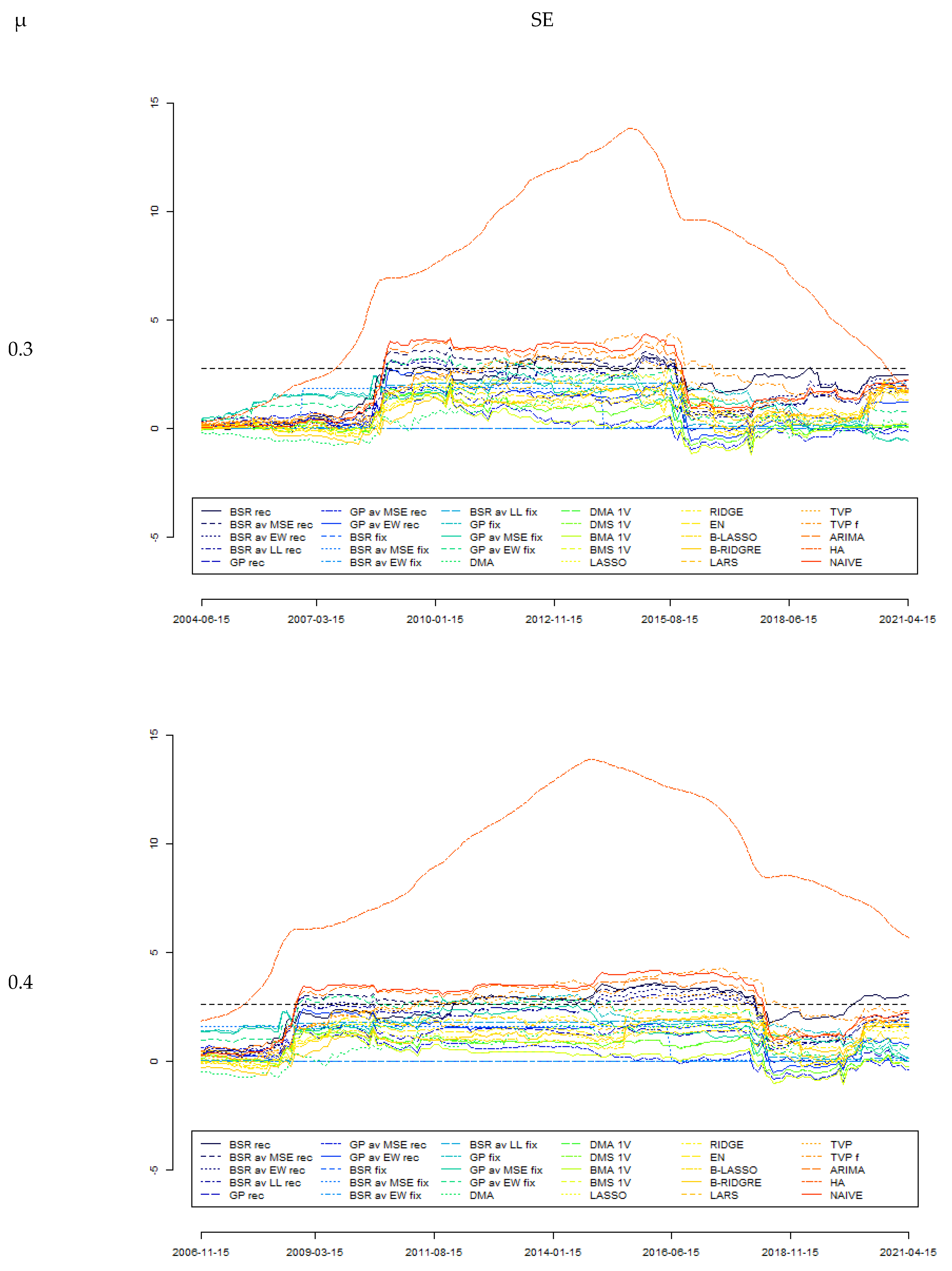
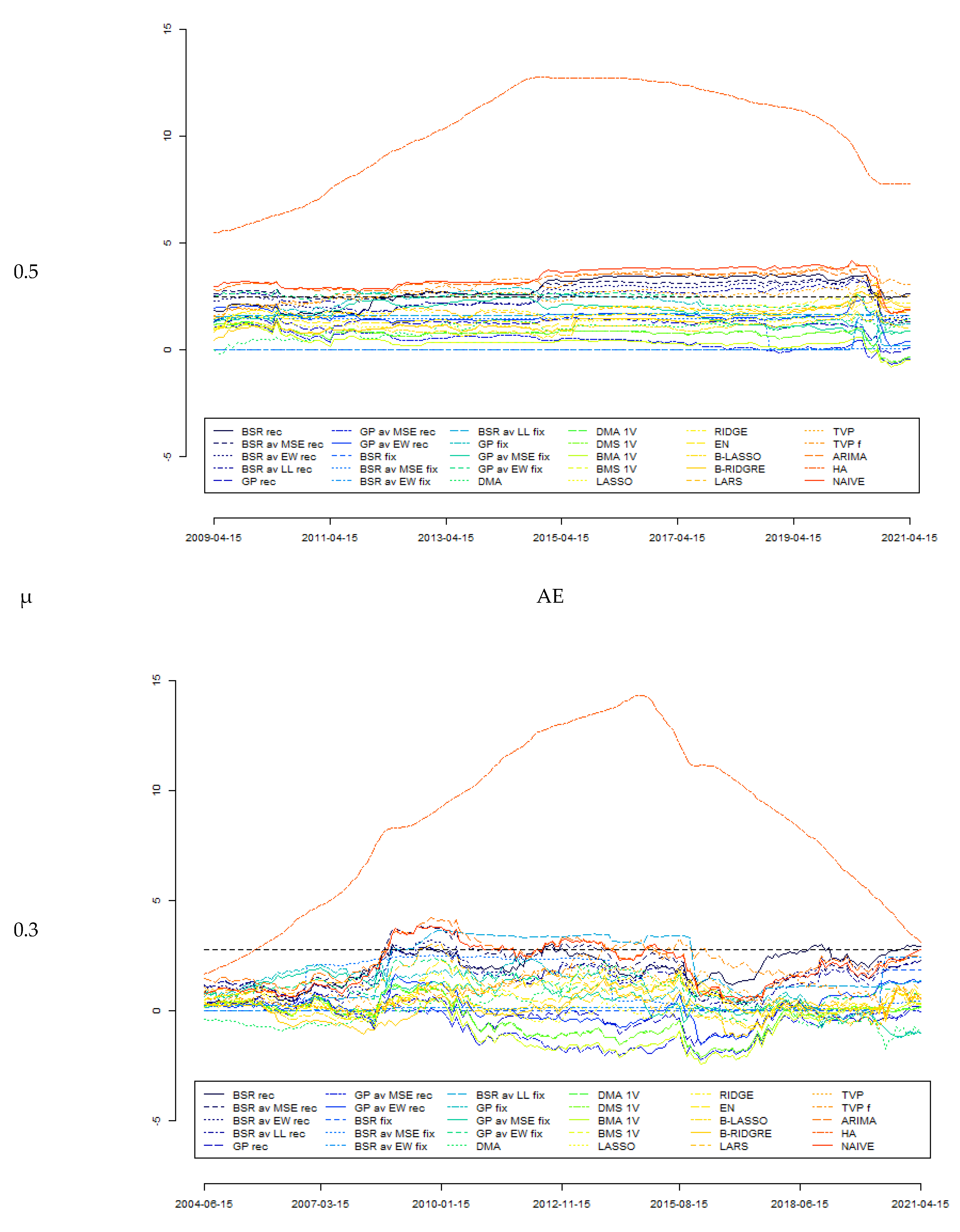
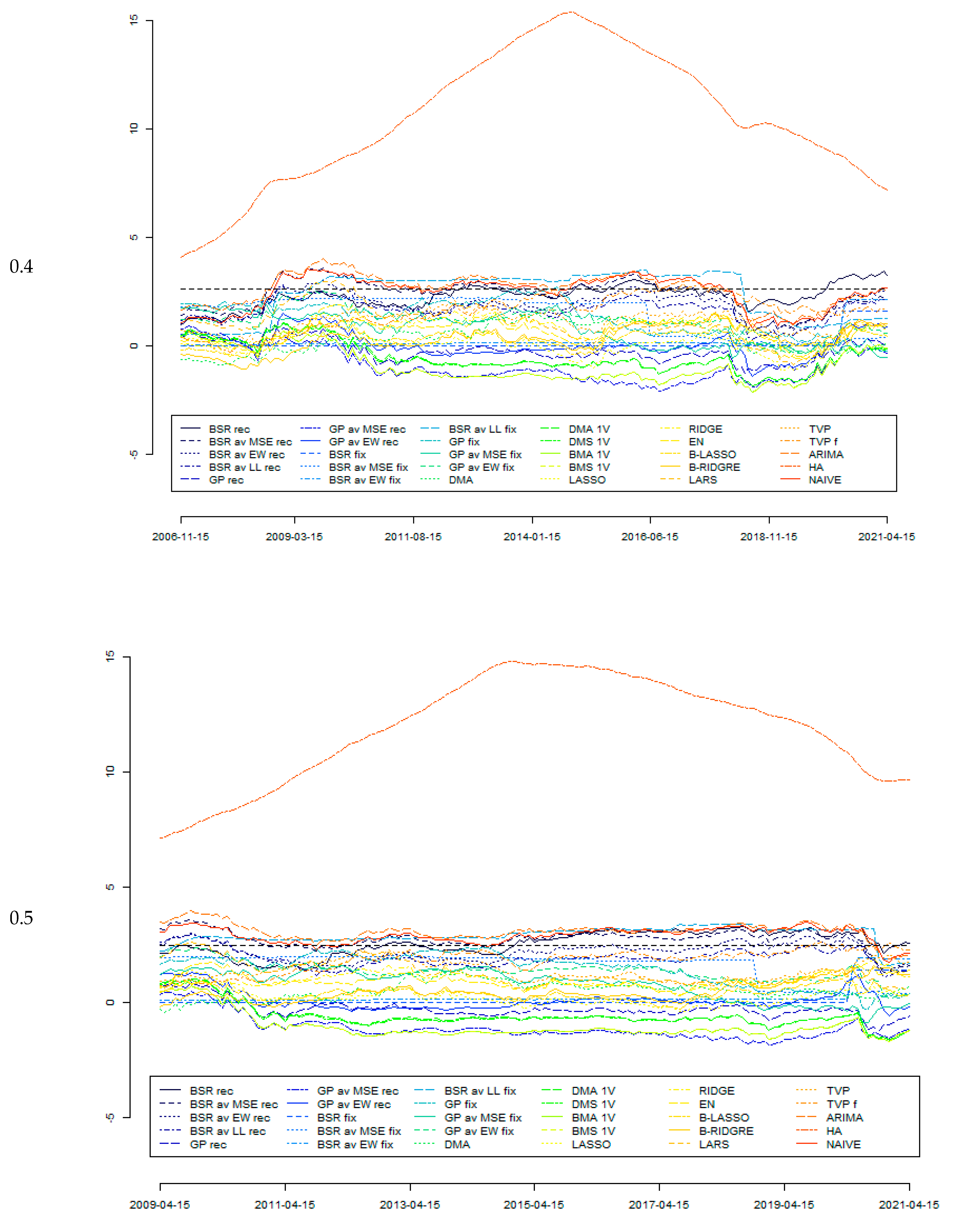
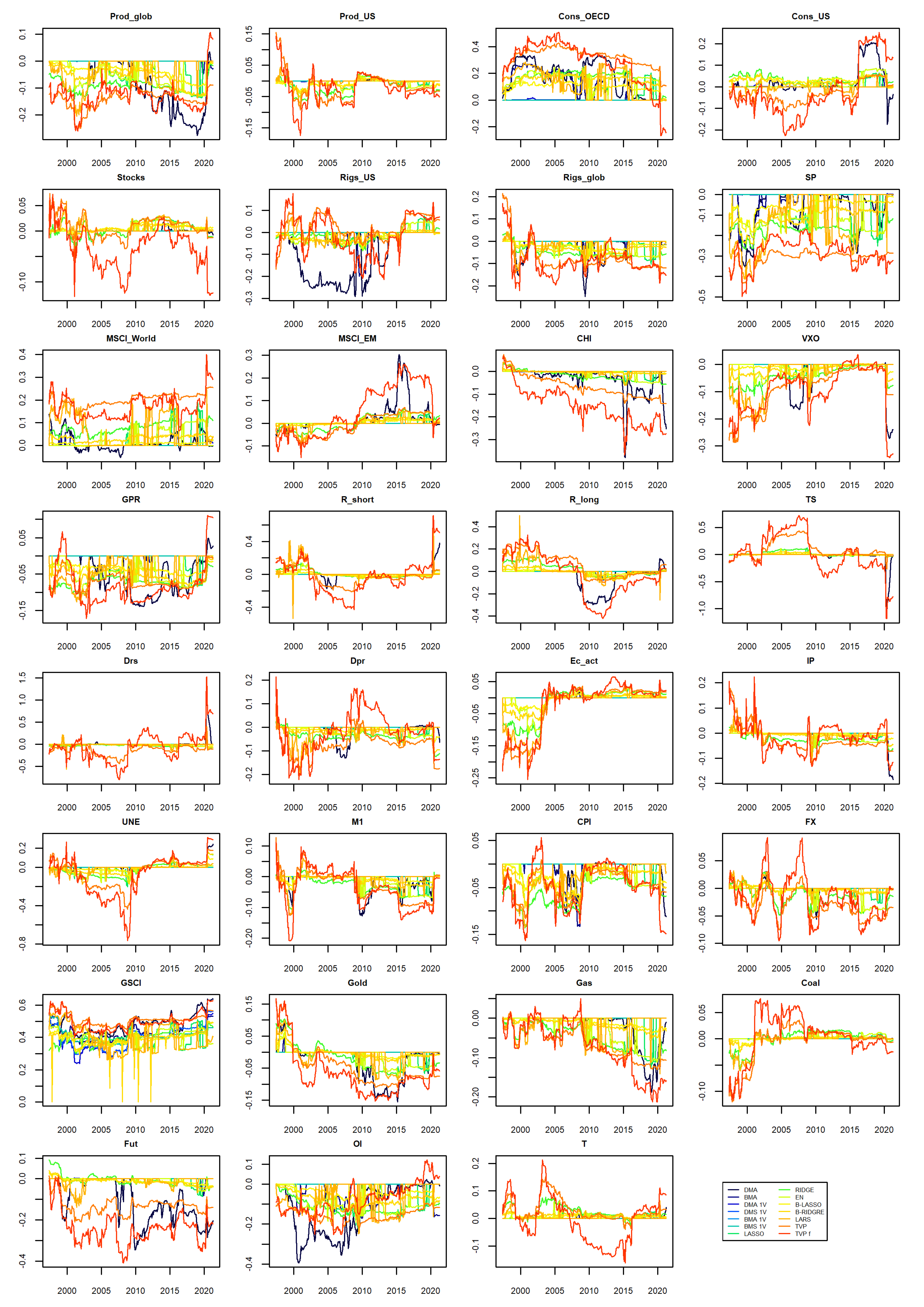
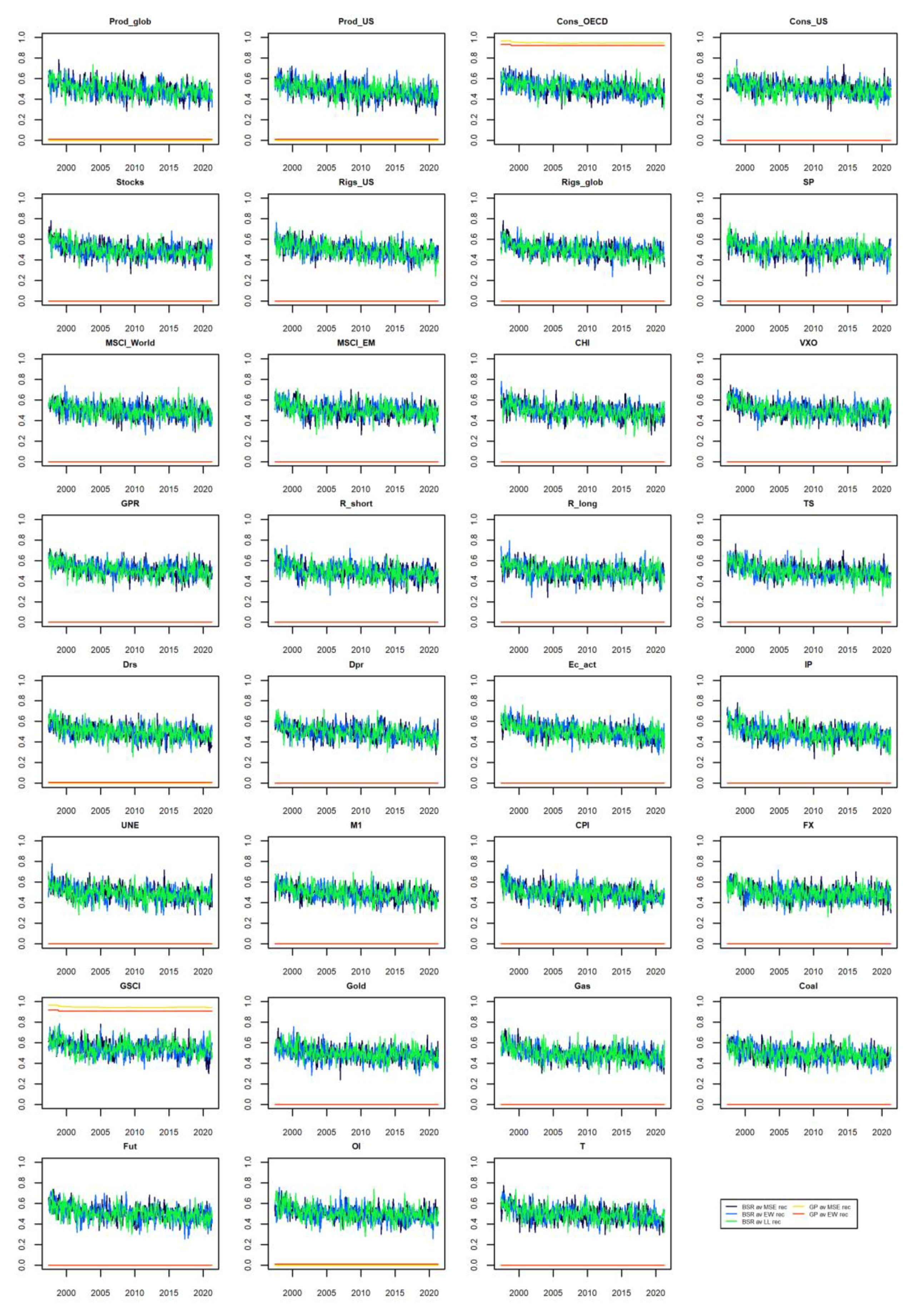
Table 1.
Variables used in this research.
| Variable Description | Variable Abbreviation | Transformation |
|---|---|---|
| Cushing, OK WTI Spot Price FOB (Dollars per Barrel) | WTI | 2 |
| Europe Brent Spot Price FOB (Dollars per Barrel) | Brent | 2 |
| Crude oil, Dubai ($/bbl) | Dubai | 2 |
| World production of crude oil including lease condensate (Mb/d) | Prod_glob | 3 |
| U.S. production of crude oil including lease condensate (Mb/d) | Prod_US | 3 |
| OECD refined petroleum products consumption (Mb/d) | Cons_OECD | 3 |
| U.S. Product Supplied of Crude Oil and Petroleum Products (Thousand Barrels) | Cons_US | 3 |
| U.S. Ending Stocks excluding SPR of Crude Oil and Petroleum Products (Thousand Barrels) | Stocks | 3 |
| U.S. Crude Oil Rotary Rigs in Operation (Count) | Rigs_US | 1 |
| Baker Hughes International Rig Count | Rigs_glob | 1 |
| S&P 500 | SP | 2 |
| MSCI WORLD (DEVELOPED MARKETS, Standard, Large+Mid Cap, USD) | MSCI_World | 2 |
| MSCI EM | MSCI_EM | 2 |
| Chinese Stock Markets | CHI | 2 |
| VXO (Month-end Closing Values) | VXO | 0 |
| GPR | GPR | 0 |
| U.S 3-Month Treasury Bill: Secondary Market Rate, Percent, Monthly, Not Seasonally Adjusted (TB3MS) | R_short | 0 |
| Long-Term Government Bond Yields: 10-year: Main (Including Benchmark) for the United States, Percent, Monthly, Not Seasonally Adjusted (IRLTLT01USM156N) | R_long | 0 |
| Term Spread | TS | 0 |
| Default Return Spread | Drs | 0 |
| Dividend-To-Price Ratio | Dpr | 0 |
| Kilian Index | Ec_act | 0 |
| U.S. Industrial Production Index, Index 2012 = 100, Monthly, Seasonally Adjusted (INDPRO) | IP | 3 |
| U.S. Unemployment Rate, Percent, Monthly, Seasonally Adjusted (UNRATE) | UNE | 0 |
| U.S. Real M1 Money Stock, Billions of 1982-84 Dollars, Monthly, Seasonally Adjusted | M1 | 2 |
| Consumer Price Index for All Urban Consumers: All Items in U.S. City Average, Index 1982–1984 = 100, Monthly, Seasonally Adjusted (CPIAUCSL) | CPI | 2 |
| Real Narrow Effective Exchange Rate for United States, Index 2010 = 100, Monthly, Not Seasonally Adjusted (RNUSBIS) | FX | 2 |
| S&P GSCI Commodity Total Return Index | GSCI | 2 |
| Gold (ozt/U.S. Dollar, XAUUSD) | Gold | 2 |
| Natural gas, US (Henry Hub spot price, Louisiana, $/mmbtu) | Gas | 2 |
| Coal, Australian ($/mt) | Coal | 2 |
| Cushing, OK Crude Oil Future Contract 1 (Dollars per Barrel) | Fut | 2 |
| Dollar Open Interest | OI | 2 |
| Working’s T-index | T | 0 |
0–no transformation: Yt → Yt; 1–12-month difference: Yt → Yt –Yt−12; 2–logarithmic difference: Yt → log(Yt)–log(Yt−1); 3–12-month logarithmic difference: Yt → log(Yt)–log(Yt−12); t denoted the time index.
Table 2.
Descriptive statistics.
| Variable | Mean | Standard Deviation | Median | Min | Max | Skewness | Kurtosis |
|---|---|---|---|---|---|---|---|
| WTI | 46.71 | 28.70 | 39.34 | 11.31 | 133.90 | 0.77 | −0.49 |
| Brent | 48.17 | 32.26 | 39.36 | 9.80 | 133.90 | 0.81 | −0.50 |
| Dubai | 45.90 | 31.67 | 34.82 | 10.05 | 131.20 | 0.80 | −0.54 |
| Prod_glob | 70,870.00 | 7335.00 | 72,640.00 | 56,970.00 | 84,610.00 | −0.04 | −1.14 |
| Prod_US | 7069.00 | 1941.00 | 6482.00 | 3974.00 | 12,860.00 | 1.22 | 0.74 |
| Cons_OECD | 46,550.00 | 2805.00 | 47,040.00 | 34,970.00 | 52,710.00 | -0.67 | 0.56 |
| Cons_US | 579,400.00 | 42,390.00 | 583,000.00 | 440,700.00 | 671,600.00 | −0.33 | −0.45 |
| Stocks | 1,079,000.00 | 123,800.00 | 1,050,000.00 | 861,200.00 | 1,453,000.00 | 1.10 | 0.46 |
| Rigs_US | 494.40 | 370.20 | 358.50 | 108.00 | 1596.00 | 1.46 | 1.27 |
| Rigs_glob | 2293.00 | 679.00 | 2113.00 | 1016.00 | 3900.00 | 0.59 | −0.68 |
| SP | 1329.00 | 800.70 | 1205.00 | 288.90 | 4181.00 | 1.02 | 0.71 |
| MSCI_World | 1209.00 | 532.90 | 1169.00 | 423.10 | 2939.00 | 0.60 | −0.18 |
| MSCI_EM | 667.60 | 331.20 | 551.50 | 132.70 | 1348.00 | 0.18 | −1.43 |
| CHI | 44,910.00 | 26,810.00 | 41,470.00 | 2274.00 | 141,100.00 | 0.40 | -0.12 |
| VXO | 19.91 | 8.31 | 18.00 | 7.87 | 61.38 | 1.64 | 3.92 |
| GPR | 87.89 | 66.29 | 65.52 | 23.74 | 545.30 | 2.82 | 12.00 |
| R_short | 2.77 | 2.39 | 2.36 | 0.01 | 8.82 | 0.44 | −0.92 |
| R_long | 4.49 | 2.11 | 4.35 | 0.62 | 9.36 | 0.27 | −0.87 |
| TS | 1.72 | 1.11 | 1.66 | −0.53 | 3.76 | 0.03 | −1.09 |
| Drs | 3.10 | 1.34 | 3.22 | 0.36 | 5.93 | −0.04 | −1.19 |
| Dpr | −1.45 | 0.28 | −1.50 | −2.03 | −0.76 | 0.36 | −0.49 |
| Ec_act | 3.41 | 60.12 | -5.03 | −159.80 | 190.60 | 0.77 | 0.86 |
| IP | 88.06 | 13.64 | 92.52 | 60.59 | 104.20 | −0.83 | −0.74 |
| UNE | 5.90 | 1.71 | 5.50 | 3.50 | 14.80 | 1.28 | 2.25 |
| M1 | 1041.00 | 1057.00 | 715.30 | 614.10 | 7100.00 | 4.82 | 23.16 |
| CPI | 194.10 | 40.75 | 192.80 | 121.20 | 266.80 | −0.02 | −1.28 |
| FX | 108.00 | 10.02 | 104.90 | 92.94 | 133.30 | 0.51 | −1.03 |
| GSCI | 3601.00 | 1627.00 | 3114.00 | 1350.00 | 10560.00 | 1.17 | 1.22 |
| Gold | 773.50 | 502.00 | 431.80 | 255.80 | 1974.00 | 0.63 | −1.10 |
| Gas | 3.60 | 2.15 | 2.87 | 1.19 | 13.52 | 1.72 | 3.53 |
| Coal | 57.91 | 30.17 | 49.44 | 22.25 | 180.00 | 1.02 | 0.46 |
| Fut | 46.74 | 28.70 | 39.41 | 11.31 | 134.00 | 0.76 | −0.49 |
| OI | 89,360,000,000.00 | 92,030,000,000.00 | 38,860,000,000.00 | 3,703,000,000.00 | 29,680,000,0000.00 | 0.64 | −1.12 |
| T | 1.08 | 0.04 | 1.08 | 1.01 | 1.24 | 0.61 | 0.11 |
Table 3.
Stationarity tests.
| Variable | ADF Stat. | ADF p-Val. | PP Stat. | PP p-Val. | KPSS Stat. | KPSS p-Val. |
|---|---|---|---|---|---|---|
| WTI | −7.8014 | 0.0100 | −238.5223 | 0.0100 | 0.0481 | 0.1000 |
| Brent | −7.7438 | 0.0100 | −244.8415 | 0.0100 | 0.0527 | 0.1000 |
| Dubai | −7.9779 | 0.0100 | −222.0210 | 0.0100 | 0.0555 | 0.1000 |
| Prod_glob | −2.8855 | 0.2033 | −44.2822 | 0.0100 | 0.5194 | 0.0373 |
| Prod_US | −3.0288 | 0.1427 | −38.8618 | 0.0100 | 1.7642 | 0.0100 |
| Cons_OECD | −3.8034 | 0.0191 | −154.1004 | 0.0100 | 1.3844 | 0.0100 |
| Cons_US | −3.9644 | 0.0110 | −175.7799 | 0.0100 | 0.5408 | 0.0325 |
| Stocks | −5.4851 | 0.0100 | −34.7983 | 0.0100 | 0.4158 | 0.0704 |
| Rigs_US | −4.8830 | 0.0100 | −20.7352 | 0.0601 | 0.2109 | 0.1000 |
| Rigs_glob | −5.8389 | 0.0100 | −28.1249 | 0.0120 | 0.3116 | 0.1000 |
| SP | −6.2031 | 0.0100 | −378.5306 | 0.0100 | 0.1225 | 0.1000 |
| MSCI_World | −6.4447 | 0.0100 | −362.0396 | 0.0100 | 0.0506 | 0.1000 |
| MSCI_EM | −7.0688 | 0.0100 | −330.9499 | 0.0100 | 0.0925 | 0.1000 |
| CHI | −6.3836 | 0.0100 | −400.7951 | 0.0100 | 0.1895 | 0.1000 |
| VXO | −3.3366 | 0.0649 | −60.1466 | 0.0100 | 0.2561 | 0.1000 |
| GPR | −4.2005 | 0.0100 | −101.6276 | 0.0100 | 1.3386 | 0.0100 |
| R_short | −3.6701 | 0.0264 | −8.5238 | 0.6332 | 4.4101 | 0.0100 |
| R_long | −3.8708 | 0.0157 | −31.7929 | 0.0100 | 6.0267 | 0.0100 |
| TS | −3.5345 | 0.0394 | −13.2871 | 0.3667 | 0.2375 | 0.1000 |
| Drs | −3.4891 | 0.0438 | −9.8452 | 0.5593 | 0.3312 | 0.1000 |
| Dpr | −1.9913 | 0.5808 | −7.0833 | 0.7138 | 1.4468 | 0.0100 |
| Ec_act | −2.4409 | 0.3910 | −22.1019 | 0.0446 | 0.7303 | 0.0108 |
| IP | −5.1379 | 0.0100 | −27.5228 | 0.0143 | 0.8551 | 0.0100 |
| UNE | −2.5066 | 0.3633 | −20.6563 | 0.0612 | 0.4055 | 0.0748 |
| M1 | −6.7871 | 0.0100 | −355.2253 | 0.0100 | 0.5388 | 0.0329 |
| CPI | −7.1785 | 0.0100 | −201.2820 | 0.0100 | 0.9009 | 0.0100 |
| FX | −7.5795 | 0.0100 | −229.7841 | 0.0100 | 0.0635 | 0.1000 |
| GSCI | −6.9948 | 0.0100 | −302.4211 | 0.0100 | 0.2696 | 0.1000 |
| Gold | −6.4954 | 0.0100 | −415.0716 | 0.0100 | 0.3922 | 0.0805 |
| Gas | −8.7395 | 0.0100 | −349.5609 | 0.0100 | 0.0580 | 0.1000 |
| Coal | −7.1172 | 0.0100 | −276.9986 | 0.0100 | 0.0523 | 0.1000 |
| Fut | −7.8003 | 0.0100 | −239.2251 | 0.0100 | 0.0533 | 0.1000 |
| OI | −7.6357 | 0.0100 | −268.1572 | 0.0100 | 0.0757 | 0.1000 |
| T | −3.1799 | 0.0915 | −43.9459 | 0.0100 | 4.4577 | 0.0100 |
Table 4.
In-sample forecast accuracy for BSR models with the different number of linear components k.
Table 4.
In-sample forecast accuracy for BSR models with the different number of linear components k.
| RMSE | MAE | MAPE | MASE | |
|---|---|---|---|---|
| k = 1 | 2.4903 | 1.3372 | 0.0637 | 1.1415 |
| k = 2 | 2.4850 | 1.3436 | 0.0641 | 1.1470 |
| k = 3 | 2.2150 | 1.1243 | 0.0559 | 0.9598 |
| k = 4 | 2.3694 | 1.2805 | 0.0623 | 1.0931 |
| k = 5 | 2.4801 | 1.3126 | 0.0624 | 1.1206 |
| k = 6 | 2.4747 | 1.3195 | 0.0629 | 1.1265 |
| k = 7 | 2.2079 | 1.1431 | 0.0560 | 0.9758 |
| k = 8 | 2.3960 | 1.2927 | 0.0619 | 1.1036 |
| k = 9 | 2.2272 | 1.0441 | 0.0507 | 0.8913 |
| k = 10 | 2.2456 | 1.0549 | 0.0509 | 0.9006 |
| k = 11 | 2.3895 | 1.2730 | 0.0615 | 1.0868 |
| k = 12 | 2.3760 | 1.2859 | 0.0621 | 1.0977 |
Table 5.
Out-of-sample forecast accuracy for all estimated models.
| RMSE | MAE | MAPE | MASE | |
|---|---|---|---|---|
| BSR rec | 5.0292 | 3.5842 | 0.0702 | 0.9686 |
| BSR av MSE rec | 4.8708 | 3.5061 | 0.0697 | 0.9475 |
| BSR av EW rec | 4.7540 | 3.4403 | 0.0683 | 0.9297 |
| BSR av LL rec | 4.8259 | 3.4482 | 0.0699 | 0.9319 |
| GP rec | 4.3060 | 3.0918 | 0.0607 | 0.8355 |
| GP av MSE rec | 4.2611 | 3.0553 | 0.0609 | 0.8257 |
| GP av EW rec | 4.4706 | 3.1509 | 0.0634 | 0.8515 |
| BSR fix | 3,062,769,697.4493 | 180,479,519.6051 | 6,319,413.9686 | 48,773,940.2698 |
| BSR av MSE fix | 18.1086 | 4.7788 | 0.0917 | 1.2914 |
| BSR av EW fix | 161.7497 | 16.5085 | 0.4792 | 4.4614 |
| BSR av LL fix | 17.7764 | 5.7118 | 0.1048 | 1.5436 |
| GP fix | 4.5174 | 3.2454 | 0.0631 | 0.8771 |
| GP av MSE fix | 4.4448 | 3.1720 | 0.0621 | 0.8572 |
| GP av EW fix | 4.6365 | 3.2708 | 0.0654 | 0.8839 |
| DMA | 4.3468 | 3.1198 | 0.0595 | 0.8431 |
| BMA | 4.2239 | 3.0905 | 0.0604 | 0.8352 |
| DMA 1V | 4.2812 | 3.0745 | 0.0606 | 0.8309 |
| DMS 1V | 4.2784 | 3.0706 | 0.0605 | 0.8298 |
| BMA 1V | 4.2532 | 3.0582 | 0.0605 | 0.8265 |
| BMS 1V | 4.2532 | 3.0582 | 0.0605 | 0.8265 |
| LASSO | 4.4275 | 3.1413 | 0.0627 | 0.8489 |
| RIDGE | 4.5231 | 3.2073 | 0.0634 | 0.8668 |
| EN | 4.4654 | 3.1804 | 0.0633 | 0.8595 |
| B-LASSO | 4.3256 | 3.1180 | 0.0615 | 0.8426 |
| B-RIDGRE | 4.3968 | 3.1407 | 0.0620 | 0.8488 |
| LARS | 4.5037 | 3.2205 | 0.0640 | 0.8703 |
| TVP | 4.7444 | 3.3103 | 0.0658 | 0.8946 |
| TVP f | 4.9461 | 3.3824 | 0.0658 | 0.9141 |
| ARIMA | 5.0009 | 3.6229 | 0.0727 | 0.9791 |
| HA | 33.2715 | 24.5524 | 0.3751 | 6.6352 |
| NAIVE | 5.2934 | 3.7003 | 0.0738 | 1.0000 |
Table 6.
Results of the Diebold–Mariano tests.
| DM Stat. | DM p-Value | DM Stat. | DM p-Value | |
|---|---|---|---|---|
| BSR rec | 3.1957 | 0.0008 | ||
| BSR av MSE rec | 2.8222 | 0.0026 | −0.6487 | 0.2585 |
| BSR av EW rec | 2.7703 | 0.0030 | −1.3763 | 0.0849 |
| BSR av LL rec | 2.8533 | 0.0023 | −0.9241 | 0.1781 |
| GP rec | 0.9791 | 0.1642 | −2.8565 | 0.0023 |
| GP av MSE rec | 0.4253 | 0.3355 | −2.9453 | 0.0017 |
| GP av EW rec | 1.6761 | 0.0474 | −2.3154 | 0.0106 |
| BSR fix | 1.0000 | 0.1591 | 1.0000 | 0.8409 |
| BSR av MSE fix | 1.0501 | 0.1473 | 1.0248 | 0.8468 |
| BSR av EW fix | 1.1502 | 0.1255 | 1.1499 | 0.8744 |
| BSR av LL fix | 1.2209 | 0.1116 | 1.1888 | 0.8822 |
| GP fix | 1.8443 | 0.0331 | −1.7019 | 0.0449 |
| GP av MSE fix | 1.5280 | 0.0638 | −1.9627 | 0.0253 |
| GP av EW fix | 2.3778 | 0.0090 | −1.4804 | 0.0699 |
| DMA | 1.0547 | 0.1462 | −2.5925 | 0.0050 |
| BMA | −3.1957 | 0.0008 | ||
| DMA 1V | 0.5766 | 0.2823 | −2.9581 | 0.0017 |
| DMS 1V | 0.5484 | 0.2919 | −2.9668 | 0.0016 |
| BMA 1V | 0.3365 | 0.3684 | −3.0684 | 0.0012 |
| BMS 1V | 0.3365 | 0.3684 | −3.0684 | 0.0012 |
| LASSO | 1.6971 | 0.0454 | −2.3414 | 0.0099 |
| RIDGE | 2.2703 | 0.0120 | −1.9027 | 0.0290 |
| EN | 1.9670 | 0.0251 | −2.1973 | 0.0144 |
| B-LASSO | 1.3271 | 0.0928 | −2.8436 | 0.0024 |
| B-RIDGRE | 1.7355 | 0.0419 | −2.4972 | 0.0065 |
| LARS | 2.2660 | 0.0121 | −2.1849 | 0.0149 |
| TVP | 2.9316 | 0.0018 | −0.9431 | 0.1732 |
| TVP f | 3.3510 | 0.0005 | −0.2645 | 0.3958 |
| ARIMA | 3.3434 | 0.0005 | −0.1295 | 0.4485 |
| HA | 11.2234 | 0.0000 | 11.1954 | 1.0000 |
| NAIVE | 3.5068 | 0.0003 | 1.0147 | 0.8444 |
Table 7.
Results of the Diebold–Mariano test for recursive (“rec”) vs. fixed (“fix”) estimations.
| DM Stat. | DM p-Value | |
|---|---|---|
| BSR | −0.6487 | 0.7415 |
| BSR av MSE | −0.5990 | 0.7252 |
| BSR av EW | −2.6759 | 0.9961 |
| BSR av LL | 1.0000 | 0.1591 |
| GP | 1.1502 | 0.1255 |
| GP av MSE | 1.9329 | 0.0271 |
| GP av EW | 2.0442 | 0.0209 |
Disclaimer/Publisher’s Note: The statements, opinions and data contained in all publications are solely those of the individual author(s) and contributor(s) and not of MDPI and/or the editor(s). MDPI and/or the editor(s) disclaim responsibility for any injury to people or property resulting from any ideas, methods, instructions or products referred to in the content. |
© 2022 by the author. Licensee MDPI, Basel, Switzerland. This article is an open access article distributed under the terms and conditions of the Creative Commons Attribution (CC BY) license (https://creativecommons.org/licenses/by/4.0/).
Share and Cite
MDPI and ACS Style
Drachal, K. Forecasting the Crude Oil Spot Price with Bayesian Symbolic Regression. Energies 2023, 16, 4. https://doi.org/10.3390/en16010004
AMA Style
Drachal K. Forecasting the Crude Oil Spot Price with Bayesian Symbolic Regression. Energies. 2023; 16(1):4. https://doi.org/10.3390/en16010004
Chicago/Turabian StyleDrachal, Krzysztof. 2023. "Forecasting the Crude Oil Spot Price with Bayesian Symbolic Regression" Energies 16, no. 1: 4. https://doi.org/10.3390/en16010004
Note that from the first issue of 2016, this journal uses article numbers instead of page numbers. See further details here.