Load-Settlement Curve and Subgrade Reaction of Strip Footing on Bi-Layered Soil Using Constitutive FEM-AI Coupled Techniques

Abstract

This study presents a hybrid Artificial Intelligence-Finite Element Method (AI-FEM) predictive model to estimate the modulus of a subgrade reaction of a strip footing rested on a bi-layered profile. A parametric study was carried out using 2D Plaxis FEM models for strip footings with width (B) and rested on a bi-layered profile with top layer thickness (h) and bottom layer thickness (H). The soil was modeled using the well-known Mohr-Coulomb’s constitutive law. The extracted load-settlement curve from each FEM model is approximated to hyperbolic function and its factors (a, b) were determined. The subgrade reaction value (Ks) is the (stress/settlement), hence (1/Ks = a·Δ + b). Both inputs and outputs of the parametric study were collected in a single database containing the geometrical factors (B, h & H), soil properties of the top and bottom layers (c, φ & γ) and the extracted hyperbolic factors (a, b). Finally, three AI techniques—Genetic Programming (GP), Evolutionary Polynomial Regression (EPR) and Artificial Neural Networks (ANN)—were implemented to develop three predictive models to estimate the values of (a, b) using the collected database. The three developed models showed different accuracy values of (50%, 65% and 80%) for (GP, EPR and ANN), respectively. The innovation of the developed model is its ability to capture the degradation of a subgrade reaction by increasing the stress (or the settlement) according to the hyperbolic formula.

1. Introduction

Strip footings are known for their application as underlain structures of buildings and pavement facilities as they are considered to be elemental strips [1,2]. The load (pressure)-settlement characteristics of these structures are of great importance due to the design parameters that the parabolic curve evaluates for constitutive modeling purposes [2,3]. Scarce land space suitable for foundation construction has compelled geotechnical experts to seek improvement methods, which is based on the available resources and the behavior of the studied soil [4]. Attempts have been made by researchers to investigate the relationship that exists between the load-settlement curves of soil foundations obtained in the field and those from laboratory studies [5]. In this effort, the analytical methods of study and the numerical techniques are correlated in order to work out the best practices to improve the carrying capacity of weak soils [5]. The load-settlement behavior of foundations in terms of failure patterns is discussed by [6,7]. Figure 1 shows the failure phases, the pressure distribution and the resultant settlement and failure pattern corresponding to general, local and punching failure modes [3].

The constitutive relations and the geometry of the foundation are studied using this load-settlement or pressure-displacement curve. It has been found that the geometry and overburden pressure of these footings depend on the “a” and “b” factors of the load-settlement relationship which states that

$$\mathrm{P}=\frac{∆}{\left(\mathrm{a}\ast ∆\right)+\mathrm{b}}$$

(1)

where P is the applied load, $∆$ is the settlement, and (a and b) are the load-settlement factors of the parabola. For the purpose of analysis and design, a working load magnitude is needed to evaluate the constitutive relation and application to the depth of the underlain soil z to which the load is applied [1,8,9]. The determination of the load-settlement factors has been increasingly important in the constitutive formulation of the solutions of the settlement and subgrade reaction of the soil-strip footing arrangement because of their dependence on the footing geometry and soil overburden pressure [3]. Stability-failure properties of foundations rested on soils have been studied using load-settlement relations and subgrade reaction behavior. The subgrade reaction (Ks) is equally related to the load-settlement constitutive relation; thus

$$\mathrm{Ks}=\frac{\mathrm{P}}{∆}=\frac{1}{\left(\mathrm{a}\ast ∆\right)+\mathrm{b}}$$

(2)

The Ks depends on the shape and geometry, including depth, z of the foundation structure; hence, its evaluation requires constitutive relations of the soil-footing interaction. Due to the use of flexible analysis in designing multiple foundations, which requires the modulus of subgrade reaction behavior of soils, the Ks has become an important parameter in the failure analysis of foundation structures. The settlement and subgrade reaction of different soil structures and arrangements have been studied previously. According to Iancu and Ionut [10], who studied the effect of foundation depth, size and shape on the subgrade reaction of cohesionless soils, it has been found that the Ks depended on the loading and the size of the loaded area. Elsamee [9] presented a summary table (

Table 1. Different proposed formulas to calculate the subgrade reaction, Ks based on elastic parameters.

No	Investigator	Year	Suggested Formula
1	Winkler	1867	$\frac{\mathrm{q}}{\mathsf{\delta }}$
2	Biot	1937	$\frac{0.95{\mathrm{E}}_{\mathrm{s}}}{\mathrm{B}\left(1-{\mathsf{\upsilon }}_{\mathrm{s}}^2\right)}{\left[\frac{{\mathrm{B}}^4{\mathrm{E}}_{\mathrm{s}}}{\left(1-{\mathsf{\upsilon }}_{\mathrm{s}}^2\right)\mathrm{EI}}\right]}^{0.108}$
3	Terzaghi	1955	${\mathrm{K}}_{\mathrm{sf}}={\mathrm{K}}_{\mathrm{sp}}\left(\frac{\mathrm{B}-{\mathrm{B}}_1}{2\mathrm{B}}\right)$
4	Vesic	1961	$\frac{0.65{\mathrm{E}}_{\mathrm{s}}}{\mathrm{B}\left(1-{\mathsf{\upsilon }}_{\mathrm{s}}^2\right)}\sqrt[12]{\frac{{\mathrm{E}}_{\mathrm{s}}{\mathrm{B}}^4}{\mathrm{EI}}}$
5	Meyerhof and Baike	1965	$\frac{{\mathrm{E}}_{\mathrm{s}}}{\mathrm{B}\left(1-{\mathsf{\upsilon }}_{\mathrm{s}}^2\right)}$
6	Selvadurai	1984	$\frac{0.65}{\mathrm{B}}\ast \frac{{\mathrm{E}}_{\mathrm{s}}}{\left(1-{\mathsf{\upsilon }}_{\mathrm{s}}^2\right)}$
7	Bowles	1988	$\frac{{\mathrm{E}}_{\mathrm{s}}}{{\mathrm{B}}_1\left(1-{\mathsf{\upsilon }}_{\mathrm{s}}^2\right){\mathrm{mI}}_{\mathrm{s}}{\mathrm{I}}_{\mathrm{F}}}$

Where q = the pressure per unit of area. $\mathsf{\delta }$ = the settlement produced by load application. B₁ = side dimension of square base used in the plate load test. B = width of footing. ksp = the value of subgrade reaction for 0.3 × 0.3 (1 ft wide) bearing plate. K_sf = value of modulus of sub-grade reaction for the full-size foundation. Es = modulus of elasticity. υ_s = Poisson’s ratio. EI = flexural rigidity of footing, m = takes 1, 2 and 4 for edges, sides and center of footing, respectively. I_S and I_F = influence factors depend on the shape of footing.

) for the evaluation of a subgrade reaction based on the effects of elastic parameters, E_s and υ_s; thus

None of the above constitutive models of subgrade reaction considered the effect of loading except the Winkler model, which considered loading per unit area (q, kN/m²) while others such as the Biot, Terzaghi, Vesic, Meyerhof and Baike, Selvadurai and Bowles considered the rigidity and Poisson relations in their models for the Ks of footings rested on soils. Various other proposed numerical models have been presented on the evaluation of the Ks which agree with the Winkler model, and these models used the Plate Loading Test (PLT) technique to arrive at their constitutive relation [9]. Mughieda et al. [11] studied the behavior of a raft foundation structure with a response to the subgrade reaction (Ks) and found that Winkler is the most popular model used to study the interaction between the Ks and foundation, which is represented by a number of springs with a significant flaw based on the lack of coupling in springs and the non-linearity of settlement in soils. It further found that the value of the Ks has an effect on the pressure distribution on the soil below the footing. Extensive related research has been studied by Ziaie–Moayed and Janbaz [12] on the parameters that affect the subgrade reaction in clayey soils in which foundation size, shape, depth and rigidity effects were observed. The size effect was verified after conducting a 3D plaxis constitutive model for the load-settlement relation and it was found that the Terzaghi equation was not suitable for low, consistent clayey soils, in terms of the shape effect on Ks, while the Terzaghi equation was found to be suitable for stiff clayey soils. The conditions for depth embedment and rigidity effects were also proposed [12]. The coupled FEM-AI technique was used to predict the lateral behavior of free head piles in a multi-layered profile, and three Artificial Intelligence (AI) techniques (GP, EPR and ANN) were used to develop the predictive models [13]. Few numerical research studies have been evidently conducted on strip foundations underlain by multilayered soil arrangements based on a subgrade reaction and load settlement curve. Previously, the assumptions in the above constitutive methods have been that the soil is homogenous and finite layered and there has been no attempt to determine the load-settlement parameters “a” and “b” which underlie the constitutive load-settlement curve model and the subgrade reaction. In the present research work, a constitutive FEM approach was used to solve, simulate and generate a database for a strip foundation rested on a multiple bi-layered soil arrangement. The multiple databases were deployed using the smart learning abilities of AI-based techniques to predict the hybrid models of the load-settlement factors (a and b).

2. Artificial Intelligence (AI) Techniques

AI is a broad scientific field that encompasses several methodologies and has numerous applications. Knowledge-based, logical, statistical, and emulating biological systems/creatures-based methods in relation to AI may all be categorized. On the other hand, applications for AI may be divided into categories for decision-making, classification, regression and optimization. The best methodologies for regression applications (such as for this research) are GP, ANN and EPR.

2.1. Genetic Algorithm GA

GA is a mathematical method for simulating the process of biological beings evolving. It hinges on the straightforward axiom “The most suitable creature will survive.” A pool of solutions for the issue under consideration, fitting criteria, and a method for creating new solutions by combining the current ones are necessary in order to make use of this optimization principle. The “Chromosome,” which is an ordered collection of genes used by biological organisms to pass on their genetic information to the next generation, is similar to how GA displays the answer as an ordered set of steps (genes). This enables GA to perform genetic operations on the solutions, such as crossover and mutation. By switching the heads and tails of the two existing solutions, the crossover mixing technique creates two new solutions from two existing ones. Mutation refers to the haphazard alteration of genetic information brought on by radiation, chemicals and copying errors; it is used by haphazardly altering a step of the solution under consideration. The algorithm cycle starts by generating a number of randomly chosen solutions for the population under consideration, assessing each one’s fitness using fitting criteria, choosing the best-fitting solutions, deleting the rest and then regaining the original population size by combining the survival solutions (using crossover and mutation procedures to generate new ones). Then, the algorithm cycle repeats. The fitting of the solutions becomes more efficient with each cycle, until it reaches an acceptable level [14].

2.2. Genetic Programming (GP)

The GA approach, which was previously discussed, is applied in GP. It depends on applying generalized additive modelling GA as a “multi-variable and structure free regression technique,” where the populations are a collection of mathematical formulas generated randomly and the fitting criterion is the “Sum of Squared Errors (SSR)” between the predicted values and the correct values of the training dataset. Each formula must be provided in genetic form (as a chromosome), rather than as a list of steps, in order to use genetic operations. The chromosome is divided into two parts: the first is a list of mathematical operators and the second is a list of variables. To create new formulae, crossover and mutation techniques are used to formulate operators and variables independently. Cycle after cycle, the SSE falls and the solutions correctness rises. Finally, a fresh (validation) dataset is used to assess the derived formula’s correctness [14].

2.3. Evolutionary Polynomial Regression EPR

Another application of GA is EPR, which is based on optimizing the number of terms in the “Traditional Polynomial Regression (TPR).” TPR is a well-known mathematical regression approach that uses the “Least Squared Error” principle to determine the best coefficient values of a polynomial function to fit a given dataset. Depending on the issue setup, the investigated polynomial may have a single or several variables (dataset). The selected polynomial degree (its maximum power) is determined by the difficulty of the issue; for basic problems, first-degree polynomial (linear) may be employed; for more sophisticated situations, second degree (quadratic), third degree (cubic), or higher degrees may be necessary. The number of polynomial terms dramatically rises as the number of variables and polynomial degree rise. For instance, a second-degree polynomial with two variables has only six terms (X² + Y² + XY + X+Y + C), whereas a third-degree polynomial with three variables has 20 terms, a fourth-degree polynomial with four variables has 70 terms, and so on. It becomes harder to apply and less practical as the number of polynomial terms rises. Therefore, utilizing the GA approach, EPR technique seeks to maximize TPR by removing the less significant words and keeping only the most useful ones. Therefore, the chromosome is comprised of a list of polynomial terms. As a result, the population (solutions) consists of a collection of polynomials, the SSE is the fitting criterion and the chromosome is made-up of a list of polynomial terms, the length of which is determined by the number of terms. The most critical words are eliminated and the less critical ones accumulate in the survival chromosomes cycle after cycle [14].

2.4. Artificial Neural Network (ANN)

Artificial Neural Network (ANN) is a catch-all term for a broad variety of AI methods that rely on emulating the actions of biological neurons. They all have nodes (cells or neurons) and connections to connect the nodes, but they differ in the way their neurons are arranged and how they are connected. One of the earliest and most common ANN types is the Multi-Layer Perceptron (MLP). It is the kind of regression problem that is most frequently employed. It is made up of several nodes placed in layers, the first layer being referred to as the “Input layer” and used to accept input values, and the last layer being referred to as the “Output layer” and used to provide output values. There are several “hidden layers” in between the input and output layers that are in charge of forecasting the outputs based on the inputs. MLP must have at least one hidden layer. Each node in a layer is linked to every other node in the layer above it and the layer below it, but the nodes in each layer are not linked to one another. The sigmoid, the hyper-tan, and the ramp functions, which are responsible for the nonlinear capabilities of the network, are the most common ones. Each connection has a significance factor called “Weight,” and each node has a triggering formula, ANN. All inputs must be scaled to a single range due to the variance in input value ranges; this process is known as “Standardization” if the input variance is divided by its standard deviation (SD), as well as “Normalization” if the inputs are scaled between (0 and 1) and “Hyper normalization” if they are scaled between (−1 to 1). Scaled inputs are transmitted through hidden layers from the input layer to the output layer. Applying a node’s activation function to the total of its inputs multiplied by the weights of the related connections yields the node’s output. The outputs must be descaled to their original resolution after the output layer. Any ANN model must be trained using a predetermined dataset; during this process, the weight values of the model’s connections are modified to anticipate the intended outputs from the inputs.

The best values for link weights might be determined using a variety of training techniques, including Back Propagation (BP), Gradually Reduced Gradient (GRG), and Genetic Algorithm GA [14].

3. Methodology

3.1. Research Program

The research plan is divided into three phases. Phase 1 involves developing 205 FEM models for strip footing rested on a bi-layered soil profile, with different configurations to determine the load corresponding to a settlement equal to 25, 50, 100 and 150 mm besides the ultimate load and settlement. Phase 2 involves calculating the values of (a and b) factors for the best fitting hyperbolic curve for the output of each FEM model and form a database that contains the configurations of each FEM model and the corresponding (a and b) values. Finlay, Phase 3 applied different AI techniques on the generated database to predict the (a and b) values using the model configurations. The next section describes in detail each phase of this research.

3.1.1. Phase 1: Constitutive FEM Models

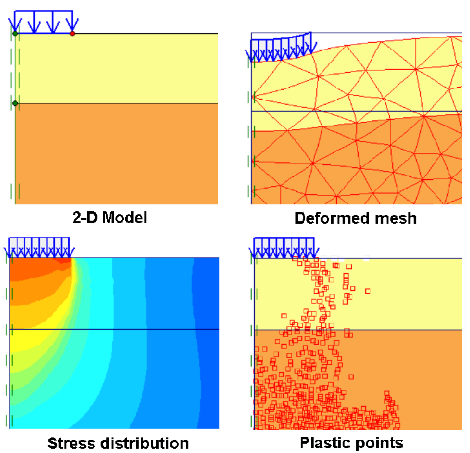
A total of 205 2D plain strain PLAXIS models were developed for a strip footing constructed on a top soil layer with thickness (h) followed by another soil layer with thickness (H). The footing width was B, as shown in Figure 2. A half model was used due to symmetry. The model dimensions in the X and Y directions were 10B. This size is large enough to prevent the effect of boundary fixation on the footing behavior. The soil elements were modeled using a 15-node element and considered the well-known Mohr–Coulomb’s constitutive law. The used parameters’ values are shown in

Table 2. Soil parameters used in the FEM models.

Soil Type	Soil Description	C (kN/m2)	φ (°)	γ (kN/m3)	E (MN/m2)	υ
S 1	loose Sand	0.0	29	16	9.0	0.350
S 2	Dense Sand	0.0	38	20	50.0	0.300
S 3	Soft Clay	25	0.0	14	1.5	0.450
S 4	Stiff Clay	100	0.0	20	10.0	0.350
S 5	Soft Silt	25	5	18	6.0	0.400
S 6	Stiff Silt	100	20	20	30.0	0.330

Where C, φ, γ′, E, υ are the cohesion, friction angle, effective unit weight, elastic modulus and Poisson’s ratio of the soil, respectively.

.

A parametric study was carried out to determine the impact of soil layers, footing dimension and overburden stress at the foundation depth on a load-settlement curve. Accordingly, a set of FEM models were developed as follows:

• Top layer (soil type S1 to soil type S6)
• Bottom layer (soil type S1 to soil type S6)
• Width of strip footing (B) (1.0 m to 5.0 m)
• Top layer thickness (h) (0.5 B to 1.0 B)
• Overburden stress (σ′v) (1.0 m to 3.0 m by the top density γ′t)

Values of the previously mentioned factors were randomly selected for each FEM model of the parametric study. Figure 3 presents a sample for the developed models and its outputs.

3.1.2. Phase 2: Evaluate (a and b) Factors, Generate the Database and Conduct Statistical Analysis

A hyperbolic formula is usually used to describe the load-settlement relation in geotechnical models such as pile load tests and plate load tests; hence, it is used in this research to describe the results of the FEM models. The best fitting hyperbolic curve for a set of results could be determined via only two factors (a and b), as shown in Figure 4.

Values of the load-settlement factors (a and b) should be selected to minimize the Sum of Squared Error (SSR) between the FEM results and the corresponding points on the hyperbolic curve. This task was carried out using a built-in function in Microsoft Excel. A complete dataset with 205 records was formed to be used by the AI techniques. Each record includes the following data:

• Cohesion, tangent of friction angle and effective density of top layer (Ct) kN/m², tan (φt) and (γ′t) kN/m³, respectively.
• Top layer thickness (h) m,
• Cohesion, tangent of friction angle and effective density of bottom layer (Cb) kN/m², tan (φb) and (γ′b) kN/m³, respectively.
• Strip footing width (B) m,
• Effective over burden stress at foundation depth (σ′v) kN/m²,
• 1000 × hyperbolic factor (a),
• 1000 × hyperbolic factor (b).

The utilized database was divided into training dataset (150 records) and validation dataset (55 records). The statistical features of the utilized dataset are shown in

Table 3. A statistical analysis of the generated database.

	Ct	tan (φt)	γ′t	h	Cb	tan (φb)	γ′b	B	σ′v	1000a	1000b
	kN/m2	-	kN/m3	m	kN/m2	-	kN/m3	m	kN/m2	kN/m2	kN/m2
Training set
Min.	0.1	0.0	14.0	0.5	0.1	0.0	14.0	1.0	18.0	0.343	0.086
Max.	100	1	20	5	100	1	20	5	54	6.340	1.880
Avg.	35.6	0.4	18.1	2.1	37.4	0.3	17.8	3.0	35.0	1.850	0.327
SD	46.0	0.3	2.2	1.3	41.2	0.3	2.4	1.6	14.7	1.610	0.272
VAR	1.29	0.87	0.12	0.61	1.10	1.02	0.13	0.54	0.42	0.870	0.832
Validation set
Min.	0.1	0.0	14.0	0.5	0.1	0.0	14.0	1.0	18.0	0.372	0.094
Max.	100	1	20	5	100	1	20	5	54	6.450	1.920
Avg.	40.6	0.3	18.4	1.8	39.5	0.3	17.6	2.7	38.4	1.880	0.347
SD	46.9	0.3	2.0	1.2	39.9	0.3	2.5	1.5	14.5	1.540	0.263
VAR	1.15	0.97	0.11	0.67	1.01	1.18	0.14	0.56	0.38	0.819	0.758

, while the correlation matrix is presented in

Table 4. Correlation matrix.

	Ct	tan (φt)	γ′t	h	Cb	tan (φb)	γ′b	B	σ′v	1000a	1000b
Ct	1.00
tan (φt)	−0.66	1.00
γ′t	0.59	0.05	1.00
h	−0.21	0.40	0.07	1.00
Cb	0.06	0.08	0.13	0.04	1.00
tan (φb)	0.09	0.02	0.02	0.05	−0.55	1.00
γ′b	0.09	0.08	0.15	0.08	0.43	0.32	1.00
B	0.02	−0.01	−0.01	0.88	0.02	0.01	0.04	1.00
σ′v	0.00	0.00	0.00	0.00	0.00	0.00	0.00	0.00	1.00
1000a	−0.12	−0.50	−0.55	−0.30	−0.20	−0.29	−0.38	−0.07	−0.18	1.00
1000b	−0.15	−0.08	−0.30	0.41	−0.19	−0.25	−0.47	0.56	0.01	0.13	1.00

. Figure 5 illustrates the histograms of both inputs and outcomes.

3.1.3. Phase 3: Predicting (a and b) Values Using AI Techniques

Three different artificial intelligence approaches were implemented to predict the hyperbolic factors (a and b) of the hyperbolic load-settlement curve of the footing using the developed dataset. The implemented approaches are Genetic programming (GP). Evolutionary Polynomial Regression (EPR) and Artificial Neural Network (ANN). The developed models predicted the (a and b) values based on geometrical dimensions h, B, the soil parameters of top layer Ct, tan (φt), γ′t, soil parameters of bottom layer Cb, tan (φb), γ′b and overburden stress σ′v. The performance of each model was measured using the Sum of Squared Errors (SSE).

4. Results and Discussion of the Predictive Models

4.1. Results Presentation

4.1.1. Model (1)—Using (ANN) Technique

A (9:10:2) layout ANN with (Hyper-Tan) activation function was trained using Back Propagation (BP) technique to predict both (a, b) values. The architecture of the generated ANN and their connation weights are showed in Figure 6 and

Table 5. Links’ Weights for the generated ANN.

		Hidden
		H1	H2	H3	H4	H5	H6	H7	H8	H9	H10
Input Layer	(Bias)	−0.96	1.31	−0.01	−1.42	−0.34	0.29	−0.39	0.17	−0.59	−1.54
	Ct	−0.27	0.63	0.75	−0.07	0.12	0.22	−0.15	−0.41	0.00	−0.1
	tan (φt)	0.31	0.36	0.41	1.16	0.17	−0.03	−0.45	0	−0.3	−0.36
	γ′t	−0.74	0.51	−0.16	−0.63	0.00	−0.28	−0.09	0.41	−0.34	−0.49
	h	0.15	−0.65	0.23	0.02	−0.04	−0.22	−0.11	0.4	−0.35	−0.15
	Cb	0.32	−0.4	0.44	0.33	−0.78	0.00	0.24	−0.06	0.08	−0.37
	tan (φb)	1.24	−0.94	0.56	0.47	−0.8	−0.32	−0.9	−0.71	−0.49	−0.27
	γ′b	−0.26	−0.83	0.26	0.61	−1.04	0.32	−1.11	−0.42	0.6	−0.17
	B	0.1	0.25	−0.15	0.15	0.37	0.5	0.02	−0.55	0.5	−0.01
	σ′v	0.45	0.26	−0.21	−0.26	−0.01	−0.24	−0.6	0.37	0.02	−0.27
		Hidden
		H1	H2	H3	H4	H5	H6	H7	H8	H9	H10	(Bias)
Output	1000a	−0.81	−1.33	−0.51	−1.28	−0.16	0.15	0.12	0.09	0.03	0.92	−0.49
	1000b	0.33	0.73	−0.07	0.78	0.62	0.04	−0.15	−0.33	0.46	0.06	−0.18

. The average errors were 16% & 25% and the (R²) values were 0.974 & 0.932. The relations between calculated and predicted values are illustrated in Figure 7c and Figure 8c.

4.1.2. Model (2)—Using GP Technique

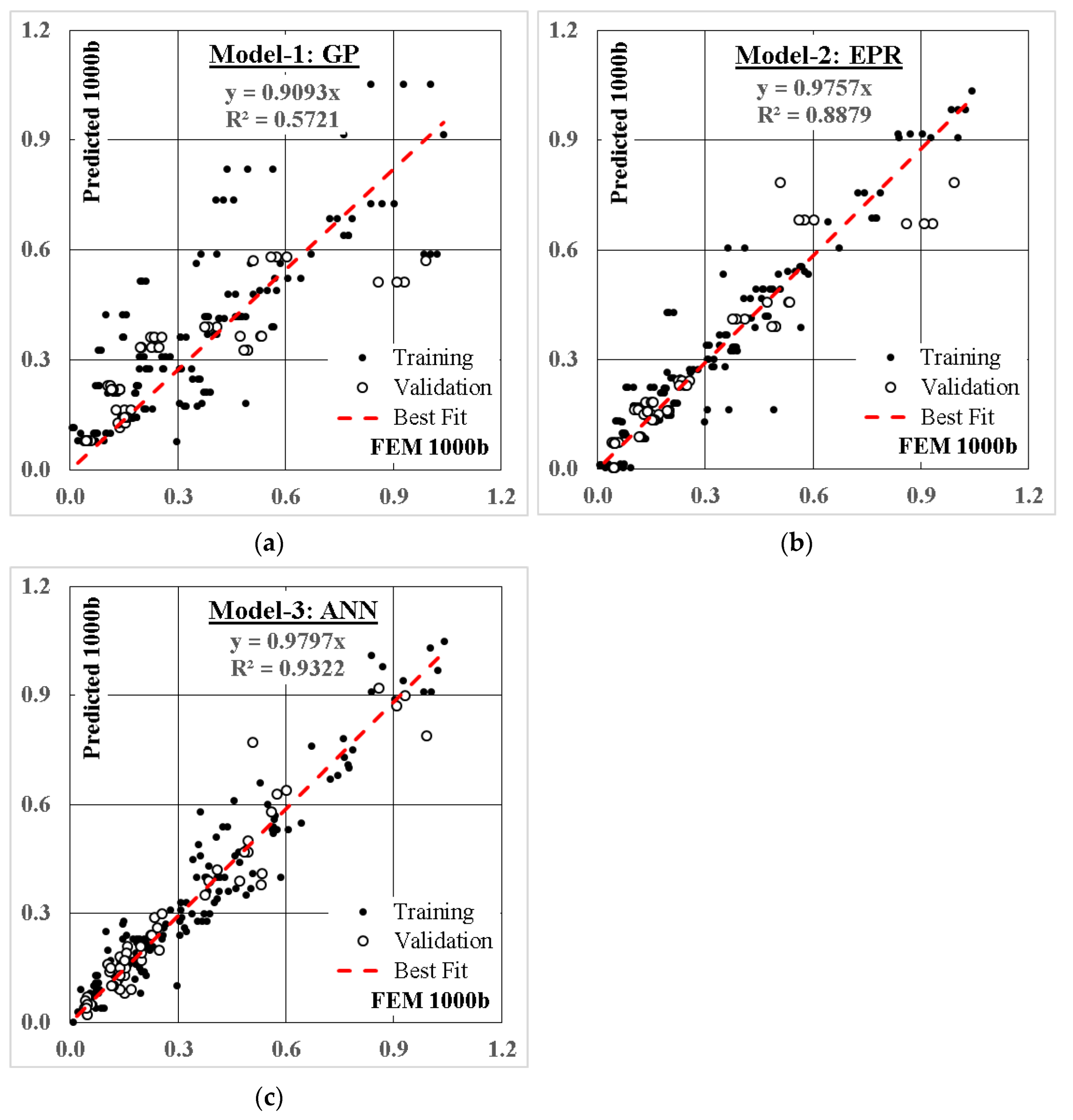
Two four levels of complexity GP models (31 gene per chromosome) were developed to predict (a and b) values of generated database records. This model was developed using a population size of 100,000 chromosomes and a survivor size of 25,000 chromosomes and 250 generations. Equations (3) and (4) present the generated formulas for (a and b), while Figure 7a and Figure 8a show their fitness. The average error and (R²) values for his model were 50%, 0.575 and 49%, 0.572, respectively.

$$1000\mathrm{a}=\frac{\frac{-{\mathsf{\gamma }}^{\prime }\mathrm{t}}{11-{\mathsf{\gamma }}^{\prime }\mathrm{b}}-\mathrm{h}·\tan \left(\mathsf{\phi }\mathrm{b}\right)+11}{7 \tan \left(\mathsf{\phi }\mathrm{t}\right)-7+{\mathsf{\gamma }}^{\prime }\mathrm{t}+\frac{\tan \left(\mathsf{\phi }\mathrm{t}\right)-{\mathsf{\gamma }}^{\prime }\mathrm{t}}{\mathrm{LN}\left({\mathsf{\sigma }}^{\prime }\mathrm{v}\right)}}$$

(3)

$$1000\mathrm{b}=\frac{2\mathrm{B}\left({\mathsf{\gamma }}^{\prime }\mathrm{b}-\mathrm{h}\right)\left(8-0.33{\mathsf{\gamma }}^{\prime }\mathrm{b}\right)}{{\mathsf{\gamma }}^{\prime }\mathrm{t} \left({\mathsf{\gamma }}^{\prime }\mathrm{b}+11\right)}$$

(4)

4.1.3. Model (3)—Using EPR Technique

A five level EPR model was generated for 9 input variables; the possible combinations are 792 terms for X⁵, 330 terms for X⁴, 120 terms for X³, 36 terms for X², 8 terms for X¹ and 1 term for X⁰ (total 1287 terms) as follows:

$$\begin{gathered} {\displaystyle \sum }_{\mathrm{i}=1}^{\mathrm{i}=2}{\displaystyle \sum }_{\mathrm{j}=1}^{\mathrm{j}=2}{\displaystyle \sum }_{\mathrm{k}=1}^{\mathrm{k}=2}{\displaystyle \sum }_{\mathrm{l}=1}^{\mathrm{l}=2}{\displaystyle \sum }_{\mathrm{m}=1}^{\mathrm{m}=2}{\mathrm{X}}_{\mathrm{i}}·{\mathrm{X}}_{\mathrm{j}}·{\mathrm{X}}_{\mathrm{k}}·{\mathrm{X}}_{\mathrm{l}}·{\mathrm{X}}_{\mathrm{m}}+{\displaystyle \sum }_{\mathrm{i}=1}^{\mathrm{i}=2}{\displaystyle \sum }_{\mathrm{j}=1}^{\mathrm{j}=2}{\displaystyle \sum }_{\mathrm{k}=1}^{\mathrm{k}=2}{\displaystyle \sum }_{\mathrm{l}=1}^{\mathrm{l}=2}{\mathrm{X}}_{\mathrm{i}}·{\mathrm{X}}_{\mathrm{j}}·{\mathrm{X}}_{\mathrm{k}}·{\mathrm{X}}_{\mathrm{l}} \\ +{\displaystyle \sum }_{\mathrm{i}=1}^{\mathrm{i}=2}{\displaystyle \sum }_{\mathrm{j}=1}^{\mathrm{j}=2}{\displaystyle \sum }_{\mathrm{k}=1}^{\mathrm{k}=2}{\mathrm{X}}_{\mathrm{i}}·{\mathrm{X}}_{\mathrm{j}}·{\mathrm{X}}_{\mathrm{k}}+{\displaystyle \sum }_{\mathrm{i}=1}^{\mathrm{i}=2}{\displaystyle \sum }_{\mathrm{j}=1}^{\mathrm{j}=2}{\mathrm{X}}_{\mathrm{i}}·{\mathrm{X}}_{\mathrm{j}}+{\displaystyle \sum }_{\mathrm{i}=1}^{\mathrm{i}=2}{\mathrm{X}}_{\mathrm{i}}+\mathrm{C} \end{gathered}$$

The most influential seven terms were determined by the GA approach. The developed mode to predict (a and b) values are presented in Equations (5) and (6), while their fitness levels are shown in Figure 7b and Figure 8b. The determination factor (R2) and average errors are 0.896, 35% and 0.888, 32%, in order. The accuracies of developed models are compared in

Table 6. Performance of the generated models.

Item	Technique	Output	SSR	Avg. Error	R2
1000a	GP	Equation (3)	178	50	0.575
	EPR	Equation (5)	87	35	0.896
	ANN	Figure 6	19	16	0.974
1000b	GP	Equation (4)	5.3	49	0.572
	EPR	Equation (6)	2.3	32	0.888
	ANN	Figure 6	1.4	25	0.932

.

$$1000\mathrm{a} =15.50-\frac{\left(22.2+{\mathsf{\gamma }}^{\prime }\mathrm{t}\right)\tan \left(\mathsf{\phi }\mathrm{t}\right){\mathsf{\gamma }}^{\prime }\mathrm{b}}{1.5 {\mathsf{\gamma }}^{\prime }\mathrm{t}}-\frac{{\mathsf{\gamma }}^{\prime }\mathrm{t} .{\mathsf{\gamma }}^{\prime }\mathrm{b} }{32.3}-\frac{208 \tan {\left(\mathsf{\phi }\mathrm{b}\right)}^2}{{\mathsf{\gamma }}^{\prime }\mathrm{b}}+\frac{12.1}{\tan {\left(\mathsf{\phi }\mathrm{b}\right)}^3}-\frac{10430}{{{\mathsf{\gamma }}^{\prime }\mathrm{b}}^3}$$

(5)

$$1000\mathrm{b} =\frac{1}{12}-\frac{\mathrm{B}\left(109 \mathrm{h}+{\mathsf{\gamma }}^{\prime }\mathrm{t}\right)}{4.9 {\mathsf{\gamma }}^{\prime }\mathrm{b}}-\frac{3.25 \tan \left(\mathsf{\phi }\mathrm{b}\right)}{{\mathsf{\gamma }}^{\prime }\mathrm{t}}-\frac{ \mathrm{B}.\mathrm{h}.{\mathsf{\gamma }}^{\prime }\mathrm{b}}{14.3}+\frac{102\mathrm{B}}{{{\mathsf{\gamma }}^{\prime }\mathrm{b}}^2}+2.5 \mathrm{B}.\mathrm{h}$$

(6)

4.2. Results Discussion

The aim of this study was to develop predictive models to generate the load-settlement curve for strip footings. Considering the hyperbolic behavior reduces the problem of predicting the values of just two parameters, (a and b). As shown in Figure 9, the hyperbolic curve could be transformed into a straight line by drawing the relation between the settlement, $∆$ and the invers of the subgrade reaction, (1/Ks =$∆/\mathrm{P}$). It could be noted that parameter (b) presents the inverse of the initial subgrade reaction (1/Kso), while parameter (a) presents the deterioration rate of the subgrade reaction while increasing the settlement [15].

In the present study, the load-settlement factors have been predicted using multiple numerical databases generated using the FEM-Plaxis 2D of a bi-layered soil bearing a strip footing of width B using the novel GP, EPR and ANN intelligent learning techniques.

Revising the developed Equations (2)–(5) shows that both Ct and Cb are missing, which indicates that cohesion has no effect of the load-settlement curve and accordingly on the subgrade reaction value.

Equations (3) and (5) indicated that increasing the effective unit weight of both the upper and lower layers increases the initial subgrade reaction (1/b), which means that raising the ground water table reduces the Kso. They also showed that increasing the foot width (B) reduces Kso, which is logical due to increasing the effective depth.

Equations (2) and (4) illustrated the complicated relation between the deterioration rate in subgrade reaction (a) and the internal friction angles (φt, φb); however, they indicated that increases both of (φt and φb) reduced the deterioration rate.

The thickness of the top layer at every trial seems to have resisted the settlement propagation to the underlying bottom layer and shows the influence of the rigidity of the soil in a multilayered arrangement on soil resistance to loading and settlement [16,17].

5. Conclusions

The fact that most available structural design software are using the subgrade reaction concept to model the soil-structure interaction is the motive to develop more accurate predictive models to determine the value of the subgrade reaction, since all the available closed form equations are valid only for single uniform layer within the elastic zone. On the other hand, this study aims to predict the full load-settlement curve of a strip footing constructed on a bi-layered profile by implementing three AI approaches: GP, EPR and ANN. These approaches were implemented for a developed database of 205 records, each record including soil parameters of the top layer (Ct), tan (φt), (γ′t), the bottom layer (Cb), tan (φb), (γ′b), geometrical dimensions (h), (B) and over burden stress (σ′v) in addition to the corresponding (a and b) hyperbolic factors. The utilized dataset was developed using the well-known Plaxis software. The outcomes of the study could be summarized as follows:

• The developed formulas using the GP technique showed a limited accuracy of 50%. All input factors were utilized, except the cohesion of both top and bottom soils (Ct), (Cb).
• EPR technique generated two seven term polynomials out of 1287 possible terms. The accuracy is better than the GP models (65%). In addition, all input factors except the overburden pressure (σ′v) and the cohesion of both the top and bottom soils (Ct), (Cb) were generated.
• Finally, ANN technique presents the best accuracy of 80% and used all the input factors. The relative importance of each factor is indicated by the size of the blocks in Figure 5, and, accordingly, all factors have almost the same effect on the load-settlement curve except (B), tan (φt) and tan (φb), which have a slightly higher effect.

According to previous points, the following are concluded:

• Both GP and EPR could not capture the influence of soil cohesion on the load-settlement curve, which gives the advantage to the ANN model.
• The developed GP model is not recommended because of its limited accuracy.
• Although the ANN model showed the best accuracy and utilised all input factors, its model is too complicated to be manually handled.
• The developed EPR model could be used for manual calculations, while the ANN model is suitable for computerized calculations
• The developed models should be used within the factor values considered in the study. The prediction accuracy must be verified beyond this range.

References

- Biswas, T.; Saran, S.; Shanker, D. Analysis of a strip footing using constitutive law. Geosciences 2016, 6, 41–44. [Google Scholar] [CrossRef]
- Onyelowe, K.C.; Mojtahedi, F.F.; Azizi, S.; Mahdi, H.A.; Sujatha, E.R.; Ebid, A.M.; Darzi, A.G.; Aneke, F.I. Innovative overview of SWRC application in modeling geotechnical engineering problems. Designs 2022, 6, 69. [Google Scholar] [CrossRef]
- Ebid, A.M.; Onyelowe, K.C.; Salah, M. Estimation of bearing capacity of strip footing rested on bilayered soil profile using FEM-AI-coupled techniques. Adv. Civ. Eng. 2022, 2022, 8047559. [Google Scholar] [CrossRef]
- Manisana, R.; Patil, N.N.; Swamy, H.M.R.; Shivashankar, R. Load-settlement characteristics of reinforced and unreinforced foundation soil. Int. J. Eng. Res. Technol. 2014, 3, 888–892. [Google Scholar]
- Nwokediuko, N.M.; Ogirigbo, O.R.; Inerhunwa, I. Load-settlement characteristics of tropical red soils of Southern Nigeria. Eur. J. Eng. Technol. Res. 2019, 4, 107–113. [Google Scholar] [CrossRef]
- Van Baars, S. Numerical check of the Meyerhof bearing capacity equation for shallow foundations. Innov. Infrastruct. Solutions 2017, 3, 9. [Google Scholar] [CrossRef]
- Ebid, A.M.; Onyelowe, K.C.; Arinze, E.E. Estimating the ultimate bearing capacity for strip footing near and within slopes using AI (GP, ANN, and EPR) techniques. J. Eng. 2021, 2021, 3267018. [Google Scholar] [CrossRef]
- Gazetas, G. Analysis of machine foundation vibrations: State of the art. Int. J. Soil Dyn. Earthq. Eng. 1983, 2, 2–42. [Google Scholar] [CrossRef]
- Elsamee, W.N.A. An experimental study on the effect of foundation depth, size and shape on subgrade reaction of cohessionless soil. Engineering 2013, 5, 785–795. [Google Scholar] [CrossRef] [Green Version]
- Iancu, B.T.; Ionut, O.T. Numerical Analyses of Plate Loading Test Numerical Analyses of Plate Loading Test; Buletinul Institutului Politehnic: Iasi, Romania, 2009; pp. 57–65. [Google Scholar]
- Mughieda, O.; Mehana, M.S.; Hazirbaba, K. Effect of soil subgrade modulus on raft foundation behavior. MATEC Web Conf. 2017, 120, 06010. [Google Scholar] [CrossRef] [Green Version]
- Ziaie-Moay, R.; Janbaz, M. Effective parameters on modulus of subgrade reaction in clayey soils. J. Appl. Sci. 2009, 9, 4006–4012. [Google Scholar] [CrossRef]
- Mahdi, H.A.; Ebid, A.M.; Onyelowe, K.C.; Nwobia, L.I. Predicting the behaviour of laterally loaded flexible free head pile in layered soil using different AI (EPR, ANN and GP) techniques. Multiscale Multidiscip. Model. Exp. Des. 2022, 5, 225–242. [Google Scholar] [CrossRef]
- Ebid, A.M. 35 Years of (AI) in geotechnical engineering: State of the art. Geotech. Geol. Eng. 2020, 39, 637–690. [Google Scholar] [CrossRef]
- Wang, C.X.; Carter, J.P. Deep penetration of strip and circular footings into layered clays. Int. J. Géoméch. 2002, 2, 205–232. [Google Scholar] [CrossRef] [Green Version]
- Carter, J.P. Solving boundary value problems in geotechnical engineering. In Pre-Failure Deformation Characteristics of Geomaterials; Jamiolkowski, M., Lancellotta, R., Lo Presti, D., Eds.; Swets & Zeitlinger: Lisse, The Netherlands, 2001. [Google Scholar]
- Merifield, R.S.; Nguyen, V.Q. Two- and three-dimensional bearing-capacity solutions for footings on two-layered clays. Géoméch. Geoengin. 2006, 1, 151–162. [Google Scholar] [CrossRef]
Figure 1.
The load-settlement behavior and failure modes.
Figure 2.
Typical configurations for the developed FEM models.
Figure 3.
A sample of the FEM model and its output.
Figure 4.
The best fitting hyperbolic load-settlement curve.
Figure 5.
Distribution histograms for inputs (in blue) and outputs (in green).
Figure 6.
The architecture of the generated ANN.
Figure 7.
Relation between predicted and calculated (1000a) values using the developed models, (a) using GP, (b) using EPR and (c) using ANN.
Figure 8.
Relation between predicted and calculated (1000b) values using the developed models, (a) using GP, (b) using EPR (c) using ANN.
Figure 9.
Hyperbolic factors (a and b).