
Do AI Models Improve Taper Estimation? A Comparative Approach for Teak
by
 , ,
, ,
Víctor Hugo Fernández-Carrillo
1,
Víctor Hugo Quej-Chi
1,*,
Hector Manuel De los Santos-Posadas
2 and
Eugenio Carrillo-Ávila
1 1
Colegio de Postgraduados Campus Campeche, Carretera Federal Haltunchén-EdznaEdzná, km 17.5, Sihochac, Municipio de Champotón C.P. 24450, Campeche, Mexico
2
Colegio de Postgraduados, Postgrado en Ciencias Forestales, Carretera México-Texcoco km 36.5, Montecillo 56230, Mexico
*
Author to whom correspondence should be addressed.
Forests 2022, 13(9), 1465; https://doi.org/10.3390/f13091465
Submission received: 6 August 2022
/
Revised: 31 August 2022
/
Accepted: 7 September 2022
/
Published: 11 September 2022
(This article belongs to the Special Issue Modelling Forest Ecosystems)
Abstract
:Correctly estimating stem diameter at any height is an essential task in determining the profitability of a commercial forest plantation, since the integration of the cross-sectional area along the stem of the trees allows estimating the timber volume. In this study the ability of four artificial intelligence (AI) models to estimate the stem diameter of Tectona grandis was assessed. Genetic Programming (PG), Gaussian Regression Process (PGR), Category Boosting (CatBoost) and Artificial Neural Networks (ANN) models’ ability was evaluated and compared with those of Fang 2000 and Kozak 2004 conventional models. Coefficient of determination (R2), Root Mean Square of Error (RMSE), Mean Error of Bias (MBE) and Mean Absolute Error (MAE) statistical indices were used to evaluate the models’ performance. Goodness of fit criterion of all the models suggests that Kozak’s model shows the best results, closely followed by the ANN model. However, PG, PGR and CatBoost outperformed the Fang model. Artificial intelligence methods can be an effective alternative to describe the shape of the stem in Tectona grandis trees with an excellent accuracy, particularly the ANN and CatBoost models.
1. Introduction
Accurate estimates of the total and commercial volume of standing Tectona grandis is essential to determine standing timber value, and the profitability of commercial forest plantations (CFP) as a business unit. Research to determine taper and variable merchantable volume has produce a diverse pool of mathematical models such as those of [1,2], who used polynomial models to model the teak bole in an experimental field in Venezuela. T. grandis is the fourth most planted forest species in Mexico with slightly over 30 thousand ha established, although with a much higher value in the international market than pine, Spanish cedar (Cedrela odorata) and eucalyptus that cover nearly 110 thousand ha according to official sources [3].
Regression models are the commonly used approach for the estimation of stem diameter [4,5,6,7]. In Mexico, most of the development and fitting of regression-based taper models has concentrated on temperate climate species, making use of systems of compatible models [8], in which taper and volume are geometrically (derivation process) and statistically (fitting under an equation system) united.
Nevertheless, in Mexico some models have been developed for T. grandis and such is the case in the study by [9] that fitted compatible volume-taper models for T. grandis grown in Campeche. However, and given the wide variety of climatic and soil conditions and silviculture in which the species is planted, a database that captures geographical, genetic and age variability is crucial to develop taper and volume estimates.
In recent years, computers have increased their processing capacity, which gives an advantage to the use of Artificial Intelligence (AI) algorithms to identify and model the relationships between complex variables at a lower computational cost.
Thus, AI models have arrived in tropical silviculture as an option to traditional regression models.
Schikowski [10] using the techniques of Artificial Neural Networks (ANN), Random Forest (RF) and k nearest neighbor (k-NN) to model the shape of the bole of Acacia mearsnsii, popularly known as black acacia; Nunes [11] also modelled with ANN and RF a complex vegetation mosaic in the biological reserve of Mogi Guacu, Brazil; likewise, Sakici [12] used the ANN approach to model taper of individual trees of Fagus orientalis and Abies nordmanniana in Karaükm, in Turkey. In another study in Poland [13], the bole shape of eight forest species was modeled using ANN and decision trees (DT) as well as the conventional method by [4] and a simple model based on linear regression; the general conclusion was that the ANN artificial intelligence method is more accurate to describe the shaft profile of the species evaluated.
Although ANNs have been widely used in forest management, including tree diameter, volume and height estimation, other AI-based algorithms have recently been proposed that have not yet been evaluated in forestry studies and have been shown to solve problems with heterogeneous features, noisy data and complex dependencies, such as Genetic Programming (GP), Gaussian Process Regression (GPR) and Category Boosting (CatBoost).
Thus, the objectives of the present study were: (1) to evaluate the capacity of four IA models, i.e., GP, GPR, CatBoost and ANN, to accurately estimate tree diameter (d) at any height of T. grandis, and (2) to compare them to the non-linear models of Kozak 2004 [4] and Fang 2000 [5], commonly used for stem characterization of the T. grandis. Applying the models to the practical activities allows obtaining an adequate estimation of the distribution of products when obtaining a CFP for this species, under development conditions in southeastern Mexico.
2. Materials and Methods
2.1. Study Area
The study area is located in the states of Campeche, Tabasco and Chiapas in southeastern Mexico where 307 trees of T. grandis were destructively sampled (Figure 1). The T. grandis plantations are growing in three humid tropical climate conditions: tropical savanna with a dry season of six months (November to April), monsoon humid tropical with a dry season of four months (January to April), and humid tropical without a dry season. The average annual temperature is higher than 22 °C and the rainfall ranges from slightly over 1000 mm annually to nearly 3000 mm. The predominant soils in these plantations are rendzinas at Campeche, vertisols and cambisols at Tabasco, and regosols and acrisols at Chiapas.
2.2. Data and Data Preprocessing
The 307 sampled trees span a diameter range at breast height (D) of 1.3 m, from 8.5 to 45 cm. The age ranges from 7.5 to 22 years, and total height (H) goes from 9 to 27 m (Table 1). The data were taken to widely encompass the variability of shape, size, and development of the species in the study zone. The diameters were taken on the bole (d) in cm at different heights (h) in m, generating 5280 pairs of height-diameter. Height-diameter pairs above branching were not taken so the length of the non-merchantable tip varies from tree to tree. A total of 3696 data pairs were used to develop all models (190 trees) and a separate set of 1584 data pairs of measured from independent trees were used to test the validity of the developed models (117 trees). Figure 2 describes the taper sampling range.
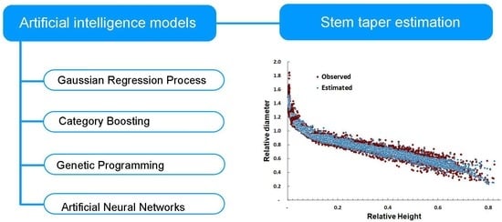
2.3. Artificial Intelligence Models
2.3.1. Genetic Programming
Genetic Programming (GP) is a technique based on the algorithms of evolution, natural selection, survival and search that allows the solution of problems through the automatic generation of algorithms and expressions [14]. These expressions are represented as a tree structure with its terminals (leaves) and nodes (functions). GP applies Genetic Algorithms (GA) on a “population” of programs or equations, that is, typically codified as tree structures. The trial programs are evaluated using an evaluation function, where programs that best adjust to the data observed are selected to later exchange information and produce better programs through crossing and mutation processes, while the worst programs are dismissed. This evolution process is repeated throughout the generations with the objective of creating a symbolic expression that best describes the data. There are five preliminary steps to solving a problem using GP. These are the determination of: (i) the set of terminals, (ii) the set of functions, (iii) the measure of evaluation, (iv) the values of the numerical parameters and the qualitative variables to control the execution, and (v) the finalization criterion to designate a result and end the execution of the algorithm [14].
The first step to use GP is to identify the set of terminals that will be used in the individual information programs of the population. The main types of sets of terminals contain the independent variables of the problem, the system state variables, and the functions without arguments. The second step is to determine the set of functions, arithmetic operations, and Boolean functions (AND, OR, NOT). The third step is to measure the aptitude, which identifies the way of evaluating how well a specific program solves a problem. Terminals and functions are the components of the programs that form the unions in the tree. The fourth step is the selection of the parameters to control the executions. The control parameters contain the size of the population, the rate of crossing, etc. The last step is the determination of the criteria to finalize the execution. In general, if the sum of the absolute differences between the results estimated with the model and those observed approach zero, then the model will be considered acceptable. Table 2 shows the optimal characteristics of the configuration of the iterative process for the training of the GP model. For the execution of the GP algorithm the HeuristicLab Version 3.3 software was used (The research group Heuristic and Evolutionary Algorithms Laboratory (HEAL), University of Applied Sciences Upper Austria).
2.3.2. Gaussian Process Regression (GPR)
The Gaussian Process Regressions (GPRs) are non-parametric probabilistic models of automatic learning used to resolve regression problems; the learning consists of inferring a function through a set of training data [15]. The GPR predicts the later probability distribution using a previous probability, and then updates the previous probability distribution by a set of data from training, in addition to providing a confidence zone for the function predicted. The GPR is fully characterized by its mean functions and covariance. This process is a natural generalization of Gaussian distribution. In this process, mean and covariance are, respectively, a vector and a matrix. There is an S dataset with n observations, where is the input vector with D dimension and is the target vector.
A Gaussian Process f(x) describes the distribution of the functions, which is why it is required to specify its mean function m(x) and covariance function k (x, x’), denoted as:
The covariance function, also known as the kernel function of the GPR, defines the degree of correlation between the exits from two entry sets , and it is the backbone of the relations between the entry variables. The mean and covariance function can be defined as Equations (2) and (3), respectively:
where denotes the mathematical expectation.
The kernel is the most significant function in the learning models based on GPR [16]; an adequate selection of the kernel function is important, since the accuracy of the model is due primarily to the covariance function selected, which determines the effectivity of the model and the accuracy of the predictions in the regression analysis [17]. In this study, an exponential square function is used as the kernel function (Equation (4)), ensuring that the predictions are invariant with changes of origin in the space of the entries [15,18].
where is the variance of the functions and specifies the maximum covariance allowed (amplitude of the function); is the length of scale, and is a strictly positive hyperparameter that determines the reach of the influence on neighboring points as they distance from each other, and is the variance of the noise of the observations. The set of hyperparameters or parameters of the covariance function is written as [17].
The hyperparameters of the covariance function are obtained through learning of the training data, using Bayesian inference techniques such as the maximization of the marginal probability.
In this study, in the implementation of the GPR technique, the algorithm was trained using the Matlab software version R2019a (Mathworks Inc., Natik, MA, USA)optimizing the kernel hyperparameters using the cross-validation technique (fold = 10) specifying their initial values for , necessary to find the final parameters of the model through the criterion of maximum marginal authenticity.
2.3.3. Category Boosting (CatBoost)
CatBoost is an automatic learning algorithm of decision trees based on a gradient boost (Gradient boosting), developed by researchers from the Russian internet company, Yandex [19], which can solve problems with heterogeneous characteristics, and data with noise and complex dependencies, as compared to other algorithms based on decision trees. Among the advantages of using CatBoost there is that it requires configuring few hyperparameters, thus avoiding the over-adjustment and obtaining more generalized models. Decision trees are used for regression, and each tree corresponds to a partition of the feature space and the output value.
This model has several advantages compared with traditional Gradient Boosting Decision Trees (GBDT) algorithms, which cope with categorical features by a method named Greedy Target Statistics (Greedy TS). To deal with categorical features during training rather than the preprocessing phase to estimate the expected and category driven target, CatBoost allows the use of a complete data set for training. According to [19], the Greedy TS strategy manages categorical features with minimum information loss. This is useful for minimizing information loss and overfitting. Given a data set D = {Xi} i = 1,…, n, where Xi = (xi, 1, …, xi, m) is a vector of m characteristics, the category of the k-th training example can be replaced by a numerical characteristic expressed in Equation (5) according to the requested TS. The substitution of a given categorical example , k can be obtained by calculating its average value with the same category value placed before in a random permutation of data set σ = (σ1, …, σn). In addition, CatBoost can combine various categorical features into a new one in a greedy way by establishing a new tree split.
where y is the objective function, P is a previous value, and is the weight of the previous value. is equal to one when , while otherwise it is equal to zero, since > 0 represents the P weight. This method contributes to reducing the noise obtained from the low frequency category.
On the other hand, CatBoost combines multiple categorical features, using a greedy way of combining all the categorical characteristics and their combinations in the current tree with all the categorical characteristics in the data set, so that CatBoost overcomes the gradient bias.
In this study, in the implementation of the CatBoost model, some of the main parameters that affect the accuracy and stability of the model were adjusted through the cross-validation technique (fold = 5); the number of iterations was fixed in 500, the maximum depth of the tree was 10, and the proportion of subsets of the data sets was fixed in 1. In the generation of the CatBoost model, Software R (R Foundation for Statistical Computing, Vienna AT) and the library Catboost [20] were used.
2.3.4. Artificial Neural Networks (ANN)
An Artificial Neural Network (ANN) is an abstract computational model that follows the behavior of the human brain [21]. The ANN can be defined as “structures made up of densely interconnected simple adaptive processing elements (called nodes or artificial neurons) capable of performing computational data processing and massively parallel knowledge representation” [22]. Each neuron in the network calculates a weighted sum by of its p entry signal hidden layers and then applies a non-linear activation function to produce an exit signal, . The form of this function is:
The most used ANN model in non-linear modelling is Multilayer Perceptron (MLP) implemented with a retro-propagation algorithm (RP). Thus, the MLP consists of one or more hidden layers. In a practical way, for the solution of non-linear regression problems, only one three-layer ANN is necessary, as shown in Figure 3, where the first layer (i) represents the input of the variables, the second layer is the hidden layer (j), and the third layer is the exit (k). Each layer is interconnected by weights Wij and Wjk, and each unit adds its entries, adding a bias or threshold term to the sum and the non-linearity, transforming the sum to produce an exit. This non-linear transformation is called a node activation function. The nodes of the exit layer tend to have linear activations. In MLP, the logistic sigmoid function (Equation (7)) and the linear function (Equation (8)) are generally used in the hidden and exit layer, respectively.
where is the weighted sum of the entry and is the entry to the exit layer.
The procedure to update the synaptic weight through the Backpropagation (BP) algorithm refers to the way in which the error calculated in the exit side propagates backward from the exit to the hidden layer(s) and finally to the entry layer [23]. The error is minimized after several cycles of training called seasons.
During each cycle, the network reaches a specific level of accuracy. Generally, the error estimator that is used here is the sum of the square error (SSE), together with the BP procedure. Likewise, a second algorithm must be chosen during the training phase that updates the weights in each cycle.
The selection of an appropriate training algorithm, the transference function, and the number of neurons in the hidden layer are fundamental characteristics of the ANN model.
In this study, for the implementation of the ANN model, a structure of three layers such as the one shown in Figure 3 was used. Likewise, the configuration was chosen that offered the best result in the study carried out by [12], where the number of neurons in the hidden layer was fixed at 10; in the hidden and exit layer the functions of logistic sigmoid (Equation (7)) and linear (Equation (8)) transference were chosen, respectively. The ANN model was trained using the RP algorithm and the Levenberg–Marquardt (LM) algorithm to update the weights in the nodes.
The ANN model was trained and validated using the Matlab® software version R2019a (Mathworks Inc, Natik MA, USA).
In general, for the training and verification of the tapering models using the artificial intelligence techniques, 70% of the data were used for the training and 30% to verify the models. On the other hand, in all the AI models, the used variables to estimate the diameter (d) of the tree stem at different heights (h) were diameter at breast height (D), height at diameter and total height (H).
2.4. Non-Linear Regression Models
In this study two well-known and efficient non-linear taper models were fitted by ordinary least squares. These models are broadly used and were selected, considering their goodness of fit and complexity. The Fang 2000 model [5] was chosen based on geometric properties (segmentation) while the Kozak 2004 [4] was selected based on performance in accurately describing taper. These models were also used by [12] where artificial neural networks models were superior in fit when compared with geometric non-linear models. Table 3 shows Equations (9) and (10) of the models selected.
These models were fitted using the statistical software SAS version 9.3 (SAS Institute, Cary, NC, USA). through the MODEL procedure to obtain the regression and goodness of fit parameters using the full information maximum likelihood (FIML) method of maximum authenticity. Both [5,24] point out that the adjustment with FIML homogenizes and minimizes the standard error of the parameters in the system.
During the fitting, auto-correlation problems were corrected with a continuous auto-regressive structure CAR (2) [6], which considers the distance between two consecutive measurements of the commercial height in each of the trees;. The structure that is added to the model is the following:
where:
is the ordinary residual in tree i,
for j > 1 and for j = 1,
is the auto-regressive parameter of order i, and
is the separation distance from j to j−1 observation within each tree, .
The auto-regressive structure was included in the MODEL procedure of SAS/ETS that allows the dynamic updating of residuals. The Durbin–Watson (DW) test suggests that the autocorrelation was overcome in the final fit of the models [25].
2.5. Goodness of Fit of the Models
The goodness of the AI and regressions models was measured based on statistics that include: Determination Coefficient (R2; Equation (12)), Root-Mean-Square Error (RMSE; Equation (13)), Mean Bias Error (MBE; Equation (14)) and Mean Absolute Error (MAE; Equation (15)).
where:
are the estimated, average and observed values, respectively, and n is the number of observations. As an evaluation criterion for the goodness-of-fit statistical criteria, it was assumed that the best fit is obtained when R2 is closest to unity and the other criteria are closest to zero.
3. Results and Discussion
As observed in Table 4 based on the goodness of fit criterion of the models, between the two conventional equations evaluated in diameter estimation, the Kozak’s model shows better results (R2 = 0.985, RMSE = 1.070, MAE = 0.746 and MBE = −0.063). Regarding the artificial intelligence models for estimating stem diameters, these were capable of describing the diametric profile with accuracy. Particularly, the ANN model obtained the best performance with relation to other models evaluated, followed by the CatBoost model. The GP model performed the lowest in comparison to the other artificial intelligence models. The results obtained using the ANN model were close enough to those obtained using Kozak’s model; however, in terms of the RMSE and MAE statistics the differences are negligible (Table 4).
Table 5 shows the fitted parameter estimates and their standard errors for both models where all the parameters were significant at 5%. Although Kozak 2004 is slightly superior in fit to Fang 2000, this latter includes an explicit total bole and variable merchantable model, while for Kozak 2004, it is necessary to directly obtain the volume by estimating the height h1 to a height h2, which can be executed without difficulty in a spreadsheet (numerical integrating this function).
As for the mean bias of the model as determined by the MBE statistic, in general all models tend to slightly underestimate the diameter of the teak tree.
In the case of CatBoost, GPR and ANN AI models, for the estimation of new values of Teak tree stem diameter by a third party, the file containing the trained algorithm can be embedded as a module on a Raspberry Pi or Arduino single board or use a specialized software for its execution, commonly R or Matlab. The trained algorithm file can be requested via e-mail to the corresponding author.
On the other hand, a useful characteristic of the GP AI model is that it provides an algebraic expression to estimate the stem diameter of the tree, which can be programmed in a spreadsheet (Equation (16)). The suggested equation derived from the GP approach is as follows:
One of the main advantages of AI-based models over traditional methods is that overfitting can be avoided by selecting an appropriate structure as in the case of ANNs or by adjusting internal parameters through cross-validation in CatBoost and GPR models. Another advantage of AI-based models is their capacity to model large amounts of noisy data from dynamic and non-linear systems. Their greatest disadvantage is that they requires specialized knowledge in the use of software and execution of programming codes for their implementation.
Figure 4 presents the residual distributions of predicted stem diameters obtained by all models using a set of 1584 independent data. Figure 4 also shows that the Kozak’s taper equation and ANN models visually adjust better, with their points close to zero and showing no tendency to over or underestimate. In addition, Figure 4 shows that the Kozak 2004 equation and ANN model best fit the observed data particularly in the lower stem sections. This is not the case for the Fang 2000 regression model which also shows errors in the upper part of the stem. Additionally, the ANN model has a slight advantage of accurate estimation of stem diameter at lower heights compared to the Kozak 2004 model.
Figure 5 shows the trend of bias for the six models along the stem at 10% relative height intervals. The models that showed the least bias in all height ranges were the Kozak 2004 and ANN models, while the Fang 2000 and GP models had the greatest bias near the stump. The GPR model showed a tendency to underestimate the taper especially above 60% relative height, where the base of the canopy would be.
In practice, estimates are made from 1 m stem height upwards, and a log length standard of 2.2 m is considered, so the commercial height hardly passes 60% of the total height. For this reason and for the graphic analysis of the bias, the use of the Kozak 2004 and ANN models is recommended in the estimation of stem diameters up to the commercial height.
It should be highlighted that the Fang 2000 model being a segmented model, the parameters p1 and p2 indicate the inflection points which in this case occur from nearly 6% and up to 54% of the total height, similar to what was reported by [7] for Quercus spp. trees and to what was reported by [9] who estimate the inflection points at 8% and 59%, respectively.
The results obtained by the conventional and artificial intelligence models evaluated here agree with other previous studies by [12], who performed a comparative analysis of the ANN technique on several conventional models, among them Kozak 2004 and Fang 2000 to determine the diameter of the stem of two forest species in Turkey. Similarly to our study, the Kozak 2004 model proved to be a very efficient structure to estimate taper, almost comparable to the best ANN models. No similar studies using CatBoost, GPR and GP techniques were found in the literature despite these techniques being quite efficient in model complex phenomena [10].
4. Conclusions
Among the four AI-based models, the ANN and CatBoost methods showed better performance than the GPR and GP methods.
From the two conventional models evaluated, the Kozak’s equation obtained a better performance compared to the Fang model, which is why its use is recommended to estimate the shape of the stem in T. grandis trees from forest plantations established in southeastern Mexico.
The artificial intelligence methods can be an effective alternative to describe the shape of the stem in T. grandis trees with an excellent accuracy, particularly the ANN and CatBoost models.
Author Contributions
Conceptualization, V.H.F.-C. and V.H.Q.-C.; methodology, H.M.D.l.S.-P. and V.H.Q.-C.; formal analysis, V.H.Q.-C. and E.C.-Á.; investigation, V.H.F.-C.; writing—original draft preparation, V.H.F.-C.; writing—review and editing, V.H.Q.-C. and E.C.-Á.; supervision, E.C.-Á. All authors have read and agreed to the published version of the manuscript.
Funding
This study did not receive resources to finance it.
Data Availability Statement
Not applicable.
Acknowledgments
The authors of this study would like to thank the Mexican company Santa Genoveva SAPI de CV for the information provided for the development of the evaluated models.
Conflicts of Interest
The authors declare no conflict of interest.
References
- Perez, D. Growth and Volume Equations Developed from Stem Analysis for Tectona Grandis in Costa Rica. J. Trop. For. Sci. 2008, 20, 66–75. [Google Scholar]
- Moret, A.; Jerez, M.; Mora, A. Determinación de Ecuaciones de Volumen Para Plantaciones de Teca (Tectona Grandis L.) En La Unidad Experimental de La Reserva Forestal Caparo, Estado Barinas–Venezuela. Rev. For. Venez. 1998, 42, 41–50. [Google Scholar]
- CONAFOR www.gob.mx/conafor/. Available online: https://www.gob.mx/conafor/documentos/plantaciones-forestales-comerciales-27940/ (accessed on 1 July 2020).
- Kozak, A. My Last Words on Taper Equations. For. Chron. 2004, 80, 507–515. [Google Scholar] [CrossRef]
- Fang, Z.; Borders, B.E.; Bailey, R.L. Compatible Volume-Taper Models for Loblolly and Slash Pine Based on a System with Segmented-Stem Form Factors. For. Sci. 2000, 46, 1–12. [Google Scholar]
- Quiñonez-Barraza, G.; los Santos-Posadas, D.; Héctor, M.; Álvarez-González, J.G.; Velázquez-Martínez, A. Sistema Compatible de Ahusamiento y Volumen Comercial Para Las Principales Especies de Pinus En Durango, México. Agrociencia 2014, 48, 553–567. [Google Scholar]
- Pompa-García, M.; Corral-Rivas, J.J.; Ciro Hernández-Díaz, J.; Alvarez-González, J.G. A System for Calculating the Merchantable Volume of Oak Trees in the Northwest of the State of Chihuahua, Mexico. J. For. Res. 2009, 20, 293–300. [Google Scholar] [CrossRef]
- Cruz-Cobos, F.; los Santos-Posadas, D.; Héctor, M.; Valdez-Lazalde, J.R. Sistema Compatible de Ahusamiento-Volumen Para Pinus Cooperi Blanco En Durango, México. Agrociencia 2008, 42, 473–485. [Google Scholar]
- Tamarit, U.J.C.; De los Santos Posadas, H.M.; Aldrete, A.; Valdez Lazalde, J.R.; Ramírez Maldonado, H.; Guerra De la Cruz, V. Sistema de Cubicación Para Árboles Individuales de Tectona Grandis L. f. Mediante Funciones Compatibles de Ahusamiento-Volumen. Rev. Mex. Cienc. For. 2014, 5, 58–74. [Google Scholar]
- Schikowski, A.B.; Corte, A.P.; Ruza, M.S.; Sanquetta, C.R.; Montano, R.A. Modeling of Stem Form and Volume through Machine Learning. An. Acad. Bras. Cienc. 2018, 90, 3389–3401. [Google Scholar] [CrossRef] [PubMed]
- Nunes, M.H.; Görgens, E.B. Artificial Intelligence Procedures for Tree Taper Estimation within a Complex Vegetation Mosaic in Brazil. PLoS ONE 2016, 11, e0154738. [Google Scholar] [CrossRef]
- Sakici, O.; Ozdemir, G. Stem Taper Estimations with Artificial Neural Networks for Mixed Oriental Beech and Kazdaği Fir Stands in Karabük Region, Turkey. Cerne 2018, 24, 439–451. [Google Scholar] [CrossRef]
- Socha, J.; Netzel, P.; Cywicka, D. Stem Taper Approximation by Artificial Neural Network and a Regression Set Models. Forest 2020, 11, 79. [Google Scholar] [CrossRef]
- Koza, J.R. Introduction to Genetic Programming. In Proceedings of the 9th Annual Conference Companion on Genetic and Evolutionary Computation, London, UK, 7–11 July 2007; pp. 3323–3365. [Google Scholar]
- Rasmussen, C.E. Gaussian Processes for Machine Learning. In Summer School Machine Learning; Springer: Berlin/Heidelberg, Germany, 2003; pp. 63–71. [Google Scholar]
- Jamei, M.; Ahmadianfar, I.; Olumegbon, I.A.; Karbasi, M.; Asadi, A. On the Assessment of Specific Heat Capacity of Nanofluids for Solar Energy Applications: Application of Gaussian Process Regression (GPR) Approach. J. Energy Storage 2021, 33, 102067. [Google Scholar] [CrossRef]
- Samarasinghe, M.; Al-Hawani, W. Short-Term Forecasting of Electricity Consumption Using Gaussian Processes. Master’s Thesis, University of Agder, West Agdelshire, Norway, 2012. [Google Scholar]
- Williams, C.K.; Rasmussen, C.E. Gaussian Processes for Machine Learning; MIT Press: Cambridge, MA, USA, 2006; Volume 2, No. 3; p. 4. [Google Scholar]
- Prokhorenkova, L.; Gusev, G.; Vorobev, A.; Dorogush, A.V.; Gulin, A. CatBoost: Unbiased Boosting with Categorical Features. Adv. Neural Inf. Process. Syst. 2018, 31, 6638–6648. [Google Scholar]
- R Foundation for Statistical Computing. R Core Team: A Language and Environment for Statistical Computing; R Foundation for Statistical Computing: Vienna, Austria, 2022. [Google Scholar]
- Haykin, S.; Lippmann, R. Neural Networks, A Comprehensive Foundation. Int. J. Neural Syst. 1994, 5, 363–364. [Google Scholar]
- Basheer, I.A.; Hajmeer, M. Artificial Neural Networks: Fundamentals, Computing, Design, and Application. J. Microbiol. Methods 2000, 43, 3–31. [Google Scholar] [CrossRef]
- Esmaeelzadeh, S.R.; Adib, A.; Alahdin, S. Long-Term Streamflow Forecasts by Adaptive Neuro-Fuzzy Inference System Using Satellite Images and K-Fold Cross-Validation (Case Study: Dez, Iran). KSCE J. Civ. Eng. 2015, 19, 2298–2306. [Google Scholar] [CrossRef]
- Borders, B.E. Systems of Equations in Forest Stand Modeling. For. Sci. 1989, 35, 548–556. [Google Scholar]
- Durbin, J.; Watson, G.S. Testing for Serial Correlation in Least Squares Regression. I; Oxford University Press: Oxford, UK, 1992; pp. 237–259. [Google Scholar]
Figure 1.
Map of locations of sampling plots in three states of the Mexican republic.

Figure 2.
Diameter behavior of T. grandis trees in the study.

Figure 3.
Three-layer ANN structure.

Figure 4.
Residual distributions of the models (a) Kozak 2004, (b) Fang 2000, (c) ANN, (d) GPR, (e) CatBoost, (f) GP.
Figure 4.
Residual distributions of the models (a) Kozak 2004, (b) Fang 2000, (c) ANN, (d) GPR, (e) CatBoost, (f) GP.

Figure 5.
Tendency of bias for 10% relative heights intervals along the stem.


Table 1.
Descriptive statistics of trees from the sample for tapering.
| Variable | Maximum | Mean | Minimum | Standard deviation |
|---|---|---|---|---|
| Normal diameter D with bark (cm) | 45.00 | 26.89 | 8.50 | 6.81 |
| Total height H of the tree (m) | 27.00 | 18.96 | 9.03 | 3.39 |
| Commercial height (Hc) of the tree (m) | 18.15 | 10.82 | 2.62 | 2.60 |
| Age (years) | 22.00 | 15.99 | 7.5 | 4.62 |
Table 2.
Parameters used in modelling with GP.
| Parameter | Characteristic |
|---|---|
| Size of the population | 500 individuals |
| Criterion of finishing | 100 generations |
| Maximum size of the tree | 150 nodes, 12 levels |
| Elites | 1 individual |
| Parent selection | Selection per tournament |
| Cross | Sub-tree, 90% of probability |
| Mutation | 15% of mutation rate |
| Function of evaluation | Coefficient of determination R2 |
| Symbolic functions | (+, −, ×, ÷, exp, log) |
| Symbolic terminals | Constant, weight × variable |
Table 3.
Conventional models used for the tapering model adjustment used in this study.
| Model | Expression | Number of Equation |
|---|---|---|
| Fang 2000 | I1 = 1 if p1 ≤ z ≤ p2 otherwise I1 = 0 I2 = 1 if p2 ≤ z ≤ 1 otheriwse I2 = 0 | (9) |
| Kozak 2004 | b = 1.3/H | (10) |
Notes: is stem diameter (cm) at height in m, is the diameter at breast height (cm), is the height of the stem (m), is the total height of the tree (m), k = /40,000. and are regression coefficients. There are intermediate variables that are explained in each model.
Table 4.
Summary statistics for diameter estimate along the stem (d) and DW parameter obtained by autocorrelation correction of the conventional models.
Table 4.
Summary statistics for diameter estimate along the stem (d) and DW parameter obtained by autocorrelation correction of the conventional models.
| Model | R2 | RMSE (cm) | MBE (cm) | MAE (cm) | DW |
|---|---|---|---|---|---|
| Kozak2004 | 0.985 | 1.070 | −0.063 | 0.746 | 2.055 |
| Fang2000 | 0.974 | 1.405 | −0.125 | 1.120 | 2.053 |
| CatBoost | 0.978 | 1.299 | −0.038 | 0.920 | - |
| GPR | 0.978 | 1.314 | −0.010 | 0.952 | - |
| ANN | 0.985 | 1.085 | −0.082 | 0.751 | - |
| PG | 0.977 | 1.343 | −0.098 | 0.964 | - |
Table 5.
Parameters estimated and standard errors of the conventional models of tapering evaluated.
| Fang 2000 | Kozak 2004 | |||
|---|---|---|---|---|
| Parameter | Estimation | Standard Error | Estimation | Standard Error |
| a0 | 0.000068 | 2.181 × 10⁻⁸ | 1.223695 | 0.0385 |
| a1 | 1.928423 | 2.507 × 10⁻⁷ | 0.990858 | 0.0063 |
| a2 | 0.854570 | 0.08590 | −0.05868 | 0.0132 |
| b1 | 2.259 × 10⁻⁶ | 2.181 × 10⁻⁸ | 0.124234 | 0.0546 |
| b2 | 9.93 × 10⁻⁶ | 2.507 × 10⁻⁷ | −1.10823 | 0.0765 |
| b3 | 0.000034 | 2.264 × 10⁻⁷ | 0.406955 | 0.0151 |
| b4 | - | - | 7.265247 | 0.5388 |
| b5 | - | - | 0.113903 | 0.00364 |
| b6 | - | - | −0.44487 | 0.0393 |
| p1 | 0.016437 | 0.000183 | - | - |
| p2 | 0.082406 | 0.00205 | - | - |
| 0.507385 | 0.0173 | 0.413999 | 0.0158 | |
| 0.159728 | 0.0109 | 0.136901 | 0.0106 | |
Publisher’s Note: MDPI stays neutral with regard to jurisdictional claims in published maps and institutional affiliations. |
© 2022 by the authors. Licensee MDPI, Basel, Switzerland. This article is an open access article distributed under the terms and conditions of the Creative Commons Attribution (CC BY) license (https://creativecommons.org/licenses/by/4.0/).
Share and Cite
MDPI and ACS Style
Fernández-Carrillo, V.H.; Quej-Chi, V.H.; De los Santos-Posadas, H.M.; Carrillo-Ávila, E. Do AI Models Improve Taper Estimation? A Comparative Approach for Teak. Forests 2022, 13, 1465. https://doi.org/10.3390/f13091465
AMA Style
Fernández-Carrillo VH, Quej-Chi VH, De los Santos-Posadas HM, Carrillo-Ávila E. Do AI Models Improve Taper Estimation? A Comparative Approach for Teak. Forests. 2022; 13(9):1465. https://doi.org/10.3390/f13091465
Chicago/Turabian StyleFernández-Carrillo, Víctor Hugo, Víctor Hugo Quej-Chi, Hector Manuel De los Santos-Posadas, and Eugenio Carrillo-Ávila. 2022. "Do AI Models Improve Taper Estimation? A Comparative Approach for Teak" Forests 13, no. 9: 1465. https://doi.org/10.3390/f13091465
Note that from the first issue of 2016, this journal uses article numbers instead of page numbers. See further details here.