1. Introduction
The world’s population growth has taken the planet to unsustainable levels of pollution, mainly caused by the industrialization of the developing world. To solve this problem we need technological changes; aiming to solve this problem, humans have developed alternative ways of producing electrical and mechanical power, to be used in the industry. One direction where these sort of policies can be applied is to alternative sources of electrical energy, ones that limit carbon emissions [
1].
In this direction, one of the most important renewable, less polluting, sources of electrical energy is wind energy. One of the problems in using this energy is its incorporation into the electrical network, due to the intermittency [
2,
3] and the difficult controllability of the main power source, turbulent wind [
4]. On the other hand, the amount of energy produced by wind power is a function of the wind speed. The challenge is to integrate this intermittent power source into the electricity grid.
We find two main streams of work in the literature regarding wind speed forecasting. One is the meteorology (or physical) approach to model and predict the state of the atmosphere [
5,
6,
7]. This approach is based on the spatial (i.e., geographical) distribution of the wind features. Those models take into consideration factors like shelter from obstacles, local surface roughness, effects of orography, wind speed change and scaling, etc. (see [
8,
9]). Those works, mainly based on partial differential equations (PDE), were developed since the early 50’s; J. Charney called those PDE Primitive Equations [
10].
The other main stream of work is based on what has been defined as Time Series Analysis. This stream of work was initiated by Yule [
11], Slutsky [
12], and Wold [
13], and made popular by Box and Jenkins [
14]. A time series is a series of data points (commonly expressing the magnitude of a scalar variable) indexed in time order. A time series is a discrete sequence taken at successive equally spaced points in time.
Within the area of Time Series Analysis, there is plenty of work based on statistics, and more recently, based on artificial intelligence and machine learning techniques. Techniques like Artificial Neural Networks [
15,
16,
17,
18], Support Vector Machines [
19,
20,
21,
22], Nearest Neighbors [
23,
24], Fuzzy Systems [
25,
26,
27,
28], and recently Deep Learning [
29,
30], have been used to model and forecast Time Series.
The study of probabilistic forecasting methods is also an important research of interest that would allow to implement wind forecasting methods in real energy production market scenarios [
31]. It could provide useful information to decision-making to maximize the rentability of wind power production, e.g., information about the future error probability distribution to know the risk of bidding certain power output. Zhang et al. [
31] classifies the probabilistic approaches in three categories according to the uncertainty representation: probabilistic (e.g., [
4,
32,
33]), risk index (e.g., [
34,
35]), and space time scenario forecasts [
36,
37,
38].
One contribution of this article is to present a performance comparison of Time Series forecasting techniques using Statistical and Artificial Intelligence methods. The methods included in this study were tested and their performances compared using two data sets, 10 Russian time series and 10 data sets from a network of weather stations located in the state of Michoacan, Mexico. The forecasting horizon used in the experiments was to predict the wind speed one day ahead for 10 days, using those time series. Note that methods that won with this data sets under this forecasting scenario may not be the winners using a different data set or forecasting horizon.
We compare one of the simplest non-linear forecasting models (NN—Nearest Neighbors), with its equivalent statistical counterpart such as ARIMA (AutoRegressive Integrated Moving Average). Based on experimental results, we show that the simple Non-linear model outperforms the statistical model ARIMA when we compare forecast accuracy for non-linear time series. Taking NN as the base model, we report the accuracy of a set of NN based models composed by a deterministic version of NN. We present a non-deterministic version (NNDE—Nearest Neighbors using Differential Evolution), that uses the Differential Evolution Algorithm to find the optimum time lag, , embedding dimension, m, and neighborhood radius size, , that produce the minimum forecasting error. Fuzzy Forecast (FF), which can be considered as a kind of Fuzzy NN, produces forecasts using fuzzy rules applied to the delay vectors. ANN-cGA (Artificial Neural Network using Compact Genetic Algorithms) evolves the architecture of ANN’s to minimize the forecasting error. As part of the evolved architecture, it determines the relevant inputs to the neural network forecaster. The input selection is closely related to the phase space reconstruction process. Finally, Evolving Directed Acyclic Graph (EvoDAG) evolves forecasting functions that take as arguments part of the history of the time series.
A second contribution of this article is the use of phase space reconstruction to determine the important inputs to the forecasting models. Phase space reconstruction determines the sub-sampling interval or time delay, , and the system dimension, m, using mutual information and false nearest neighbors, respectively; these parameters are used to produce the characteristic vectors known as delay vectors. These delay vectors are the input to the different models presented in this article.
When reviewing the literature, there are differences in the ranges of the time scale between different works. For example, Soman et al. [
39] use the term very short term to denote forecasting for a few seconds to 30 min in advance, short-term for 30 min up to 6 h ahead, medium-term for 6 h to one day ahead, and long-term from 1 day to a week ahead. According to their classification, this article addresses medium- and long-term forecasting; applications for these time scales, according to Soman et al., include generator online/offline decisions, operational security in day-ahead electricity market, unit commitment decisions, reserve requirements decisions, and maintenance and optimal operational cost, among others. They also present a study of different methods applied to different time scales; according to their work they conclude that statistical approaches and hybrid methods are “very useful and accurate” for medium- and long-term forecast. Therefore a performance comparison between AI methods for this particular forecast horizon offers guidance for the practitioners of the field.
The rest of the article is organized as follows:
Section 2 provides a brief analysis of the state of the art in time series analysis using the methods included in this study.
Section 3.2, describes the forecasting techniques used in the comparative analysis presented here.
Section 4 describes the data sets used in the comparative analysis, the experimental setup, and the results of the comparison. Finally,
Section 5 draws this empirical study conclusions.
2. Related Work
The study and understanding of wind speed dynamics for prediction purposes affects the performance of wind power power generation. Wind speed dynamics present a high level of potential harmful uncertainty to the efficiency of energy dispatch and management. Therefore, one of the biggest goals in wind speed forecasting is to reduce and manage the uncertainty with accurate models with the aim of increasing added value to the wind power generation.
Nevertheless, wind speed prediction is difficult to perform accurately and requires more than the traditional linear correlation-based models (i.e., Auto-Regressive Integrating Moving Average). Wind speed dynamics presents both strong chaotic and random components [
40], which must be modeled and explained from the non-linear dynamics perspective. We found in the literature a diverse collection of wind power and speed forecasting models to meet the requirements predicting at specific time horizons.
The work of Wang et al. [
2] is a comprehensive survey that organizes the forecasting models according to prediction horizons, e.g., immediate short time (8-h ahead), short term (one-day ahead), and long term (greater than one-day ahead).
L. Bramer states [
41] that for short term forecasting horizons (from 1 to 3 h ahead), statistical models are more suitable than other kinds of models. In contrast, for longer horizons, the alternative methods perform better than the pure statistical models. Our forecasting horizon (one day ahead) calls for other methods, capable to produce forecasts deeper than that into the future. That is the reason to use AI-based techniques.
Okumus and Dinler [
42] present a comprehensive review where they cite an important number of wind power and speed forecasting models, compared by standard error measures and length of the prediction horizon. The paper compares ANFIS, ANN, and ANFIS+ANN model, presenting better performance improving by 5% on average. The hybrid model presents a MAPE improvement of 25% for 24-h step ahead forecasts. Table 1 of Okumus et al.’s article provides errors obtained in the works included in their survey; unfortunately, those errors are reported for different forecasting tasks, using different error metrics. Under those conditions we cannot really compare the performance of the methods we present in this article with those presented in the articles included in the survey. It is not even clear to us the main characteristics of the data they use (e.g., sampling period, time series length, etc.); we do not know how complex the data is in those examples and forecasting accuracy depends on those factors.
Another multivariate model is proposed by Cadenas et al. [
43] for one step ahead forecasting, using Nonlinear Auto-regressive Exogenous Artificial Neural Networks (NARX). The NARX model considers meteorological variables such as wind speed, wind direction, solar radiation, atmospheric pressure, air temperature, and relative humidity. The model is compared against Auto-regressive Integrated Moving Average (ARIMA) model; NARX reports a precision improvement between 5.5% and 10%, and 12.8% for one-hour and ten-minute sample period time series.
Croonenbroeck and Ambach [
44] compare and analyze the effectiveness of WPPT (Wind Power Prediction Tool) with GWPPT (Generalized Wind Power Prediction Tool) using wind power data of 4 wind turbines located in Denmark. WPPT is also compared with Non-parametric Kernel Regression, Mycielsky’s Algorithm [
45], Auto-regressive (AR), and Vector Auto-regressive (VAR). Their experiments were performed with one and 72-step (12 h) ahead forecasting horizons with a sampling period of 10 min.
Jiang et al. [
46], present a one-day ahead wind power forecasting using a hybrid method based on the combination of the enhanced boosting algorithm and ARMA (ARMA-MS). An ARMA model is selected with parameters
and
for the AR and MA components, respectively. The ARMA-MS algorithm is based on the weighed combination of several ARMA forecasters. ARMA-MS is tested with wind power data from the east coast of the Jiangsu Province.
Despite the plethora of algorithms and models to forecast wind speed, the authors found few articles using non-linear time series theory [
47,
48]. Non-linear time series theory is useful to identify the structure and attractors, and predict time series with non-linear and potential chaotic behavior. An example is the Simple Non-Linear Forecasting Model based on Nearest Neighbors (NN) proposed by H. Kantz [
23].
Previous experimental results with synthetic chaotic time series [
49], indicate that using basic principles to reconstruct the non-linear time series in phase space, perform far better predictions than the basic statistic principles. They show that the prediction quality can be improved even more by using Differential Evolution.
3. Materials and Methods
This section describes the data sets used to test the forecasting methods presented in this article. Several forecasting techniques (developed by the authors) were selected to solve the wind speed forecasting problem. Those forecasting methods are then presented in the second subsection.
Section 4 presents a comparative analysis of those forecasting techniques; the study was designed to be as exhaustive as possible.
3.1. Data Sets
The methods included in this study were tested and their performances compared using two data sets: a selection of 10 stations from the compilation “Six- and Three-Hourly Meteorological Observations from 223 Former U.S.S.R. Stations (NDP-048)” [
50], and 10 are a subset of the network of weather stations located in the state of Michoacan, Mexico [
51]. Every data set contains wind speed measurements collected at a height of 10 m. Russian time series are sampled at 3-h periods and Mexican time series are sampled every hour.
The forecasting horizon used in the experiments was to predict the wind speed one day ahead for 10 days, using those time series. Since we are forecasting for 10 days, the last 10 days of measures of each data set were saved in the validation set; the rest of the data was used as a training set. The number of samples used for training varied depending on the time series, ranging from 875 to 25,000 samples, while the length of the validation sets were 80 and 240 for the Russian and Mexican time series, respectively.
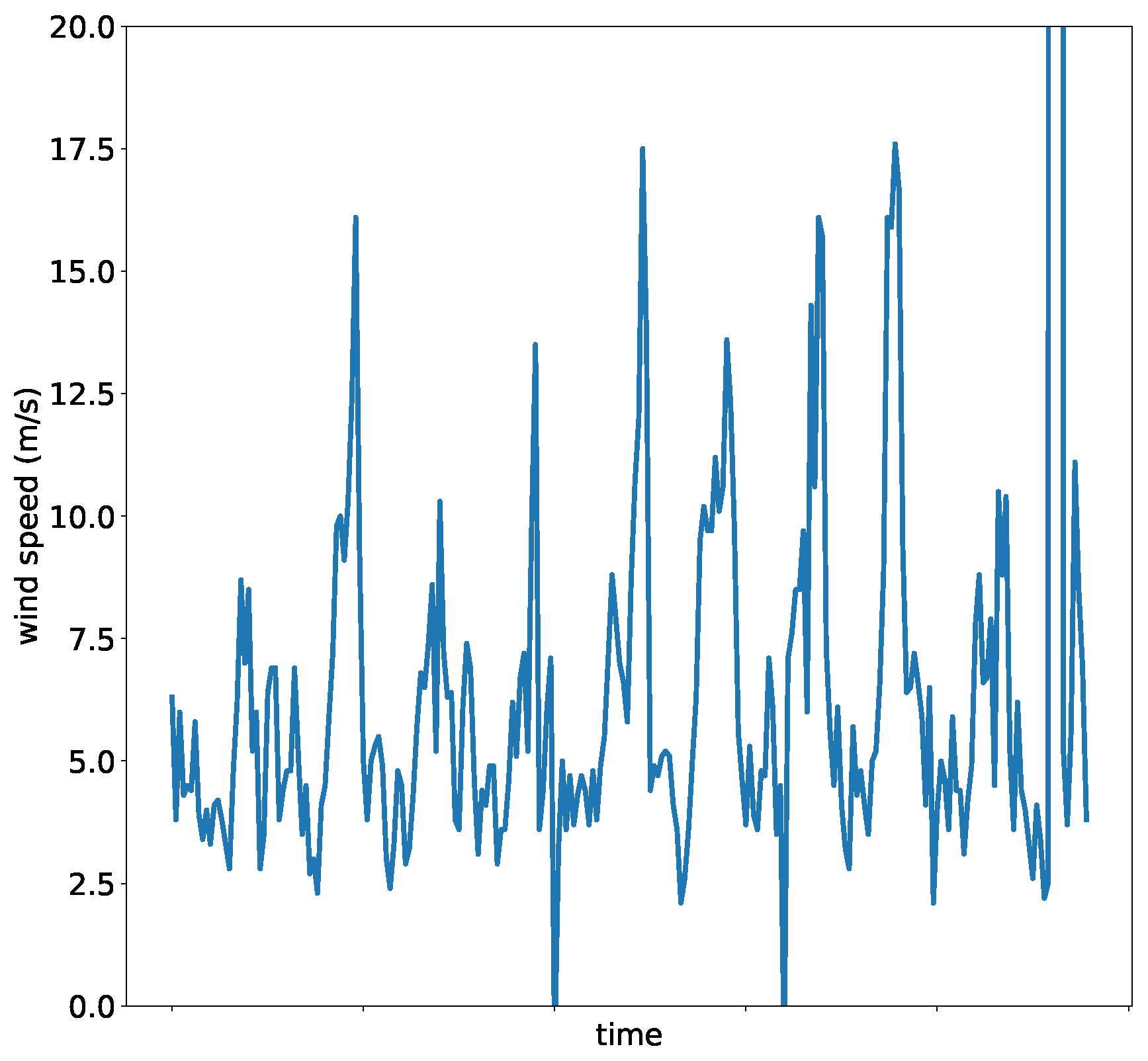
Figure 1 presents an example of the Mexican time series. For the sake of clarity, only a subset of the time series has been plotted. Given the range of wind speeds in the malpais area, it is clear that the time series presents an outlier near the end of the plotted data, where it goes well beyond 20 m/s.
These data sets were selected since they present different problems encountered in non-synthetic experimentation, most importantly: noise, outliers, data precision, and missing values. In the particular case of the Russian stations, wind speed is measured as integers with no decimals, which adds a layer of noise since the data lacks granularity. The Mexican stations have one decimal digit.
While there are practically no missing values in the Russian data sets, the Mexican data sets lack several values. Because of this, some adjustments to train the forecasters and measure their performance were necessary. Those adjustments are described in
Section 4.4.
Also, mostly in the Mexican data sets, some outliers were identified, both in the training and validation sets of some stations. As with the missing values, a few adequations were implemented in the forecasters to correctly treat these data sets.
3.2. Forecasting Techniques
This section describes the techniques used in the performance comparison, presenting the equations and algorithms that composes them. Auto-Regressive Integrated Moving Average and Nearest Neighbors are well known forecasting techniques, while Nearest Neighbors with Differential Evolution Parameter Optimization, Artificial Neural Network with Compact Genetic Algorithm Optimization, Fuzzy Forecasting, and EvoDAG are the authors’ recent contributions to the state of the art.
3.2.1. Auto-Regressive Integrated Moving Average
In time series statistical analysis, the Auto-Regressive Moving Average models (ARMA) describes a (weakly) stationary stochastic process in terms of two polynomials. The Auto-Regressive Integrated Moving Average models (ARIMA), are a generalization of ARMA models. These models fit to time series data to obtain insights of the data or to forecast future data points in the series. In some cases, these models are applied to data where there is evidence of non-stationarity (this is, where the joint probability distribution of the process is time variant).In those cases, an initial differentiation step (which corresponds to the integrated part of the model) can be applied to reduce the non-stationarity [
13].
Much empirical time series behave as if they did not have a bounded mean. Yet, they exhibit homogeneity in the sense that, parts of the time series are similar to other parts in different time lapses. The models that serve to identify non-stationary behavior can be obtained by applying adequate differences on the time series. An important class of models for which the d-th difference is a mixed stationary auto-regressive moving average process is called the ARIMA models.
The non-stationary ARIMA models are described as
, where
p,
d, and
q are non-negative integer parameters;
p is the order of the auto-regressive model,
d is the differentiation degree, and
q is the order of the moving average model [
52].
Let us define the time lag operator B such that, when applied to a time series element, it produces the previous element. I.e., . It is possible to call a time series homogeneous, non-stationary. If it is not stationary, but its first difference, , or any high-order differences produces a stationary time series, then can be modeled by an Auto-Regressive Integrated Moving Average process (ARIMA).
Hence, an
model can be written as in Equation (
1)
where
is an independent term (a constant),
and
are polynomials on
B,
is the time series at time
t, and
is the error at time
t.
After differentiation, which produces a new stationary time series, this results in an auto-regressive moving average model ARMA, which has the form shown in Equation (
2), which can be expressed using polynomials of the lag operator,
B, as shown in Equation (
3)
where
and
are the coefficients of the polynomials Φ and Θ.
3.2.2. Nearest Neighbors with Differential Evolution Parameter Optimization
Let be a time series, where is the value of variable s at time t. It is desired to obtain the forecast of consecutive values, by employing any observation available in .
By using a delay and an embedding dimension m, it is possible to build delay vectors of the form , where and . The nearest neighbors are those whose distance to is at most .
For each vector
that satisfies Equation (
4), the individual values
are retrieved.
Each of these vectors form the neighborhood with radius r around the point . It is possible to use any vector distance function to measure the distance between possible neighbors.
The forecast is the mean of the values
of every delay vector near
, expressed in Equation (
5).
The Nearest Neighbors algorithm requires that its parameters are fine tuned so it can produce accurate forecasts. Differential Evolution contributes to obtain the best parameters given an specific fitness function. This hybrid method that combines Nearest Neighbors with Differential Evolution is called NNDE [
49].
What it does is, for a stochastically generated population of individuals, each of which is encoded by a vector , a forecast is obtained for the given time series. Then, the forecasts are compared to the validation set of the time series with an error measure such as MAPE or MSE. The result is the fitness of each individual set of parameters, and the individual with the lowest fitness is the one used to evolve the population. Once this process is completed, the individual with the overall lowest error is retrieved and becomes the set of parameters to use to produce forecasts for that particular time series.
3.2.3. Fuzzy Forecasting
Fuzzy Forecasting (FF) learns a set of Fuzzy Rules (FR) designed to predict a time series behavior. FF traverses the time series analyzing contiguous windows with its next observations and formulating a rule from each one of them. Those rules take the form of Equation (
6).
where
m and
are the embedding parameters, and
are the Fuzzy Linguistic Terms (FLTs).
The FLTs are formed by dividing the time series range into overlapping intervals. By producing a higher number of FLTs, the resulting forecaster is more precise. On the other hand, the process of learning the FR is more expensive (time-wise). The FLTs overlap just enough so that every real value belongs to at least one FLT (i.e., at least one membership function is not zero). An FR (see Equation (
6)) represents the behavior of the time series in the time window where the FR is extracted from. The FR is a low resolution version of the information contained in the time series window.
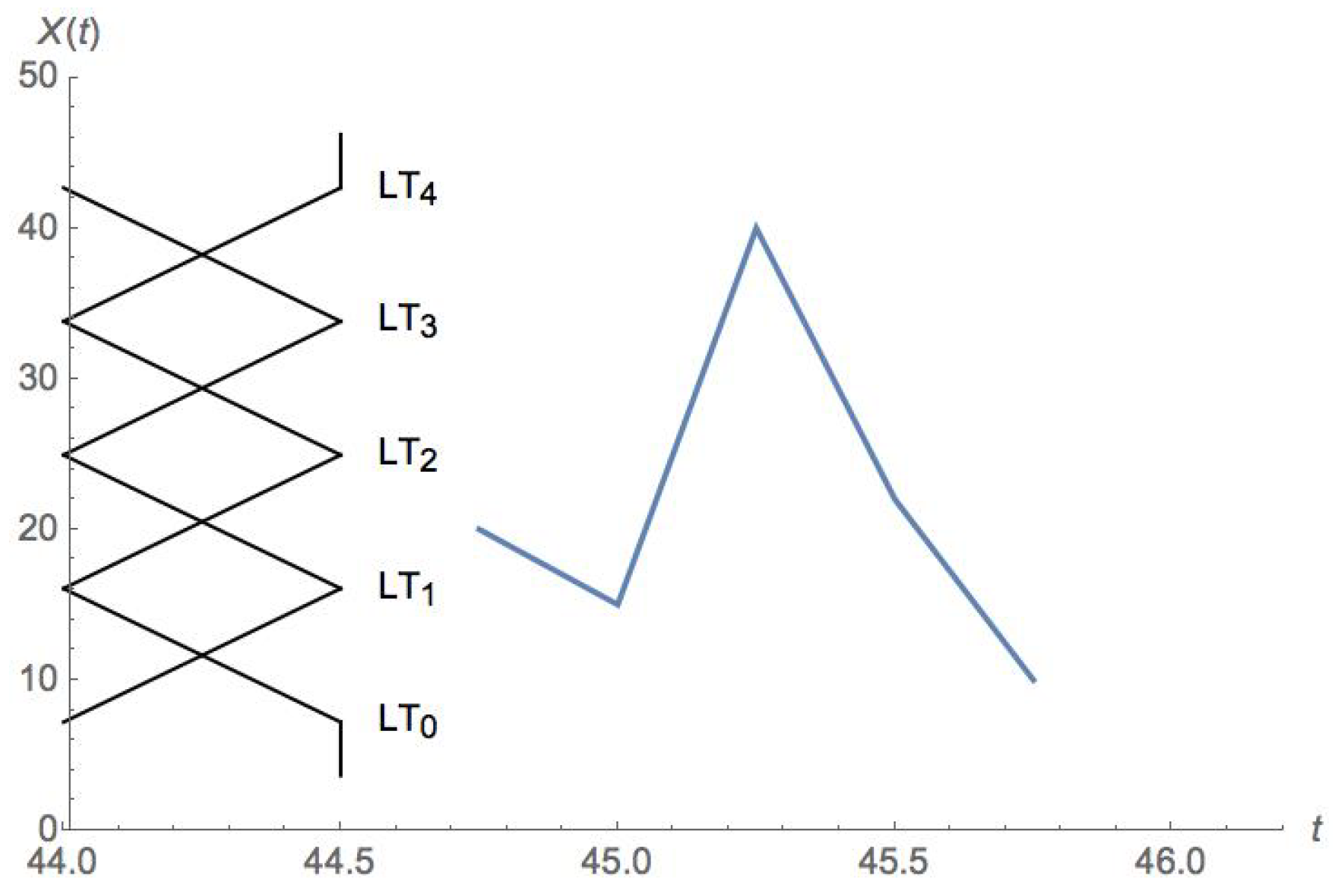
Figure 2 illustrates a delay window of a time series. The magnitudes in the time series chosen for this example range from 6 to 44. That range was evenly split to produce 5 overlapping FLTs, running along the vertical axis. The first 4 points of that delay window form the antecedents, and the last one constitutes the consequent of the produced FR. Assuming
, and that the rule will be applied at time
t, the produced FR has the form
.
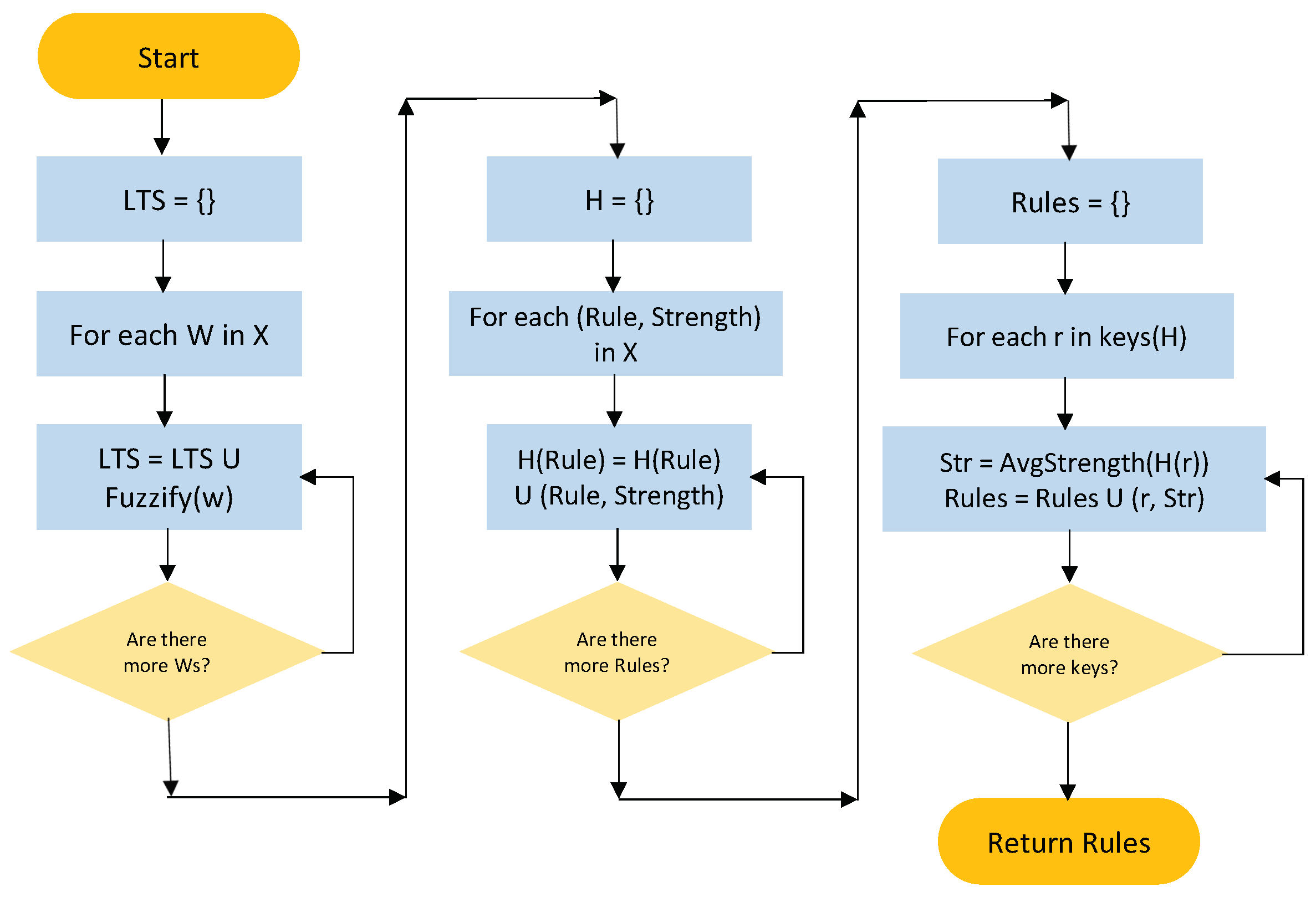
Fuzzy Forecasting has two phases: Learning and forecasting. The first phase learns the FR set from the time series.
Figure 3 shows a flow chart of the learning algorithm. Function LearnRules takes
X, a time series,
m, and
and returns the FR set learned from
X.
LearnRules has three main parts, shown in each of the columns in
Figure 3. First,
X is traversed using a sliding window, looking for patterns contained in the time series. Those sliding windows (
W) have size
m with delay
; each window is fuzzified and added to the list of Linguistic Terms,
. In the second part, those rules are traversed again, gathering them by the fuzzy form of the rule. The rules are stored in a dictionary
H of rules and their strengths. Finally, all collected rules of the same form are compiled into a single one, with the strength of the average of the set. The compiled (learned) set of rules is returned.
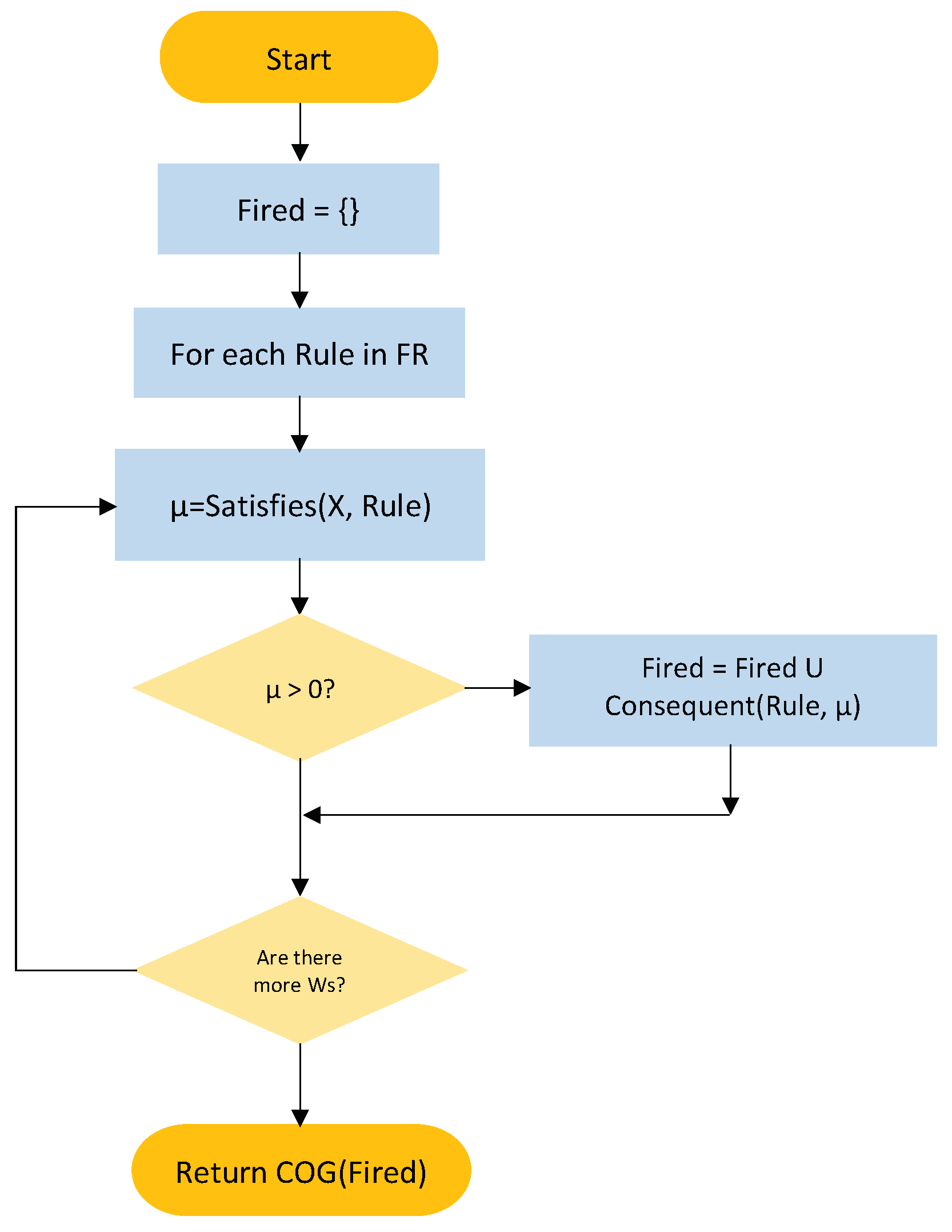
The second phase of Fuzzy Forecasting is the production of the forecasts, based on the current observation and the set of fuzzy rules produced by the learning phase. Given a FR set, forecasting uses a fuzzy version of the current state of the time series, and sends this fuzzy state to the FR to produce the predicted value. In the forecasting process, more than one rule may fire; in those cases, the result (i.e., the forecast) is defuzzified using the center of gravity method.
Figure 4 shows a flow chart of the forecasting algorithm. FuzzyForecasting produces one forecasted value, computed from the set of fuzzy rules and the delay vector formed by the last observations.
FuzzyForecasting takes the FR set, the time series, X, and the window size m. The Loop traverses FR, verifying if the fuzzy current state satisfies each fuzzy rule. When the fuzzy current state satisfies the antecedents of a rule, we say it fires. The membership of the conjunction of the memberships of the antecedents is called the rule fire strength. When a rule fires, its consequent and the firing strength are recorded in the list Fired. When all rules were traversed the fired rules’ strength is combined and defuzzified using the Center of Gravity method. The defuzzufied value, which represents the forecast value, is returned.
3.2.4. Artificial Neural Network (ANN) with Compact Genetic Algorithm Optimization
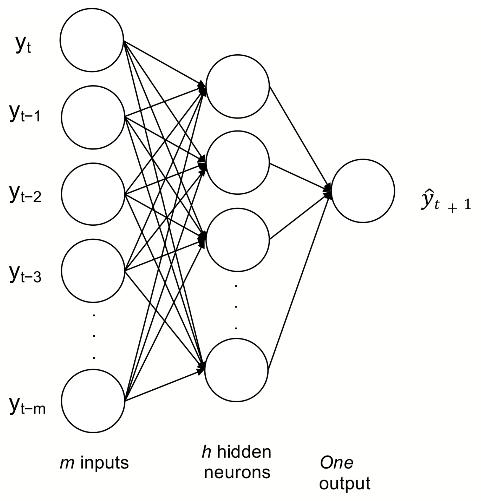
ANNs are inspired are inspired by the functioning of the human brain. They have the capacity to model a non-linear relationship between input features and expected output. The ANN used in this work is a multi layer perceptron (MLP) with three layers. The first layer receives the inputs (
m past observations), the hidden layer (one or more) which are the processing layers, and an output layer (the forecast). A sigmoid function is used as an activation function (as observed in
Figure 5) [
53].
A correct training process may result in a Neural Network Model that predicts an output value, classify an object, approximate a function, or complete a known pattern [
54].
The ANN architecture used to forecast is defined by a compact Genetic Algorithm (cGA). The cGA algorithm and the chromosome description are shown in the work of Rodriguez et al. [
55].
3.2.5. EvoDAG
EvoDAG [
56,
57] is a Genetic Programming (GP) system designed to work on supervised learning problems. It employs a steady-state evolution with tournament selection of size 2. GP is an evolutionary search heuristic with the particular feature that its search in a program space. That is, the solutions obtained by GP are problems; however, EvoDAG restricts this search space to functions. The search space is obtained by composing elements from two sets: the terminal set and the function set. The terminal set contains the inputs and, traditionally, an ephemeral random constant. On the other hand, the function set includes operations related to solve the problem. In the case of EvoDAG, this set is composed by arithmetic, transcendental, trigonometric functions, among others.
EvoDAG uses a bottom-up approach in its search procedure. It starts by considering only the inputs, and then these inputs are joined with functions of the function set, creating individuals composed by one function and their respective inputs. Then these individuals are the inputs of a function in the functions set, creating offspring which will be the inputs of another function and so on. The evolution continues until the stopping criteria are met.
Each individual is associated with a set of constants that are optimized using ordinary least squares (OLS), even the inputs are associated with a constant. For example, let be the first input in the terminal set, then the first individual created would be where is calculated using OLS. In order to depict the process of creating an individual using a function of the function set, let and be two individuals and be the addition the function selected from the function set, then the offspring is where and are obtained using OLS.
EvoDAG uses as stopping criteria early stopping, which employs part of the training set as a validation set. The validation set is used to measure the fitness of all the individuals created, and the evolution stops when the best fitness in the validation set has not been improved for several evaluations, using by default 4000. Specifically, EvoDAG splits the training set in two; the first one acts as the training set and the second as the validation set. The training set guides the evolution and is used to optimize the constants in the individuals. Finally, the model, i.e., the forecaster, is the individual that obtained the best fitness in the validation set.
EvoDAG is a stochastic procedure having as a consequence high variance. In order to reduce the variance, it was decided to create an ensemble of forecasters using bagging. Bagging is implemented considering that the training set is split in two to perform early stopping; thus, it is only necessary to perform different splits, and for each one, a model is created. The final prediction is the median of each model’s prediction.
4. Results
With the techniques described in
Section 3.2, two experiments based on the same forecasting scenario were tested. In this section we discuss the performance of the forecasters measured by the Symmetric Mean Average Percentage Error.
4.1. Auto-Correlation Analysis of the Data Sets
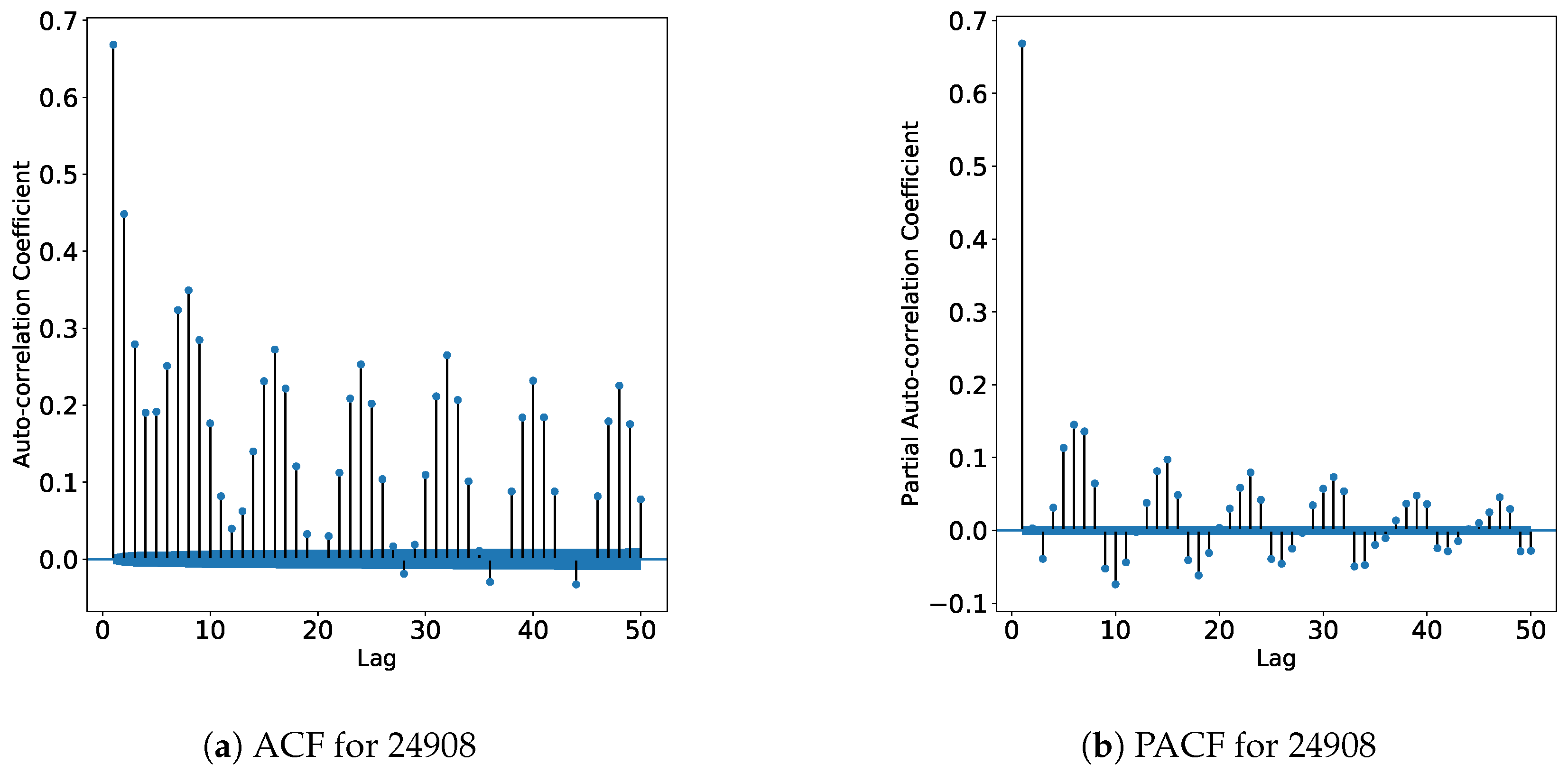
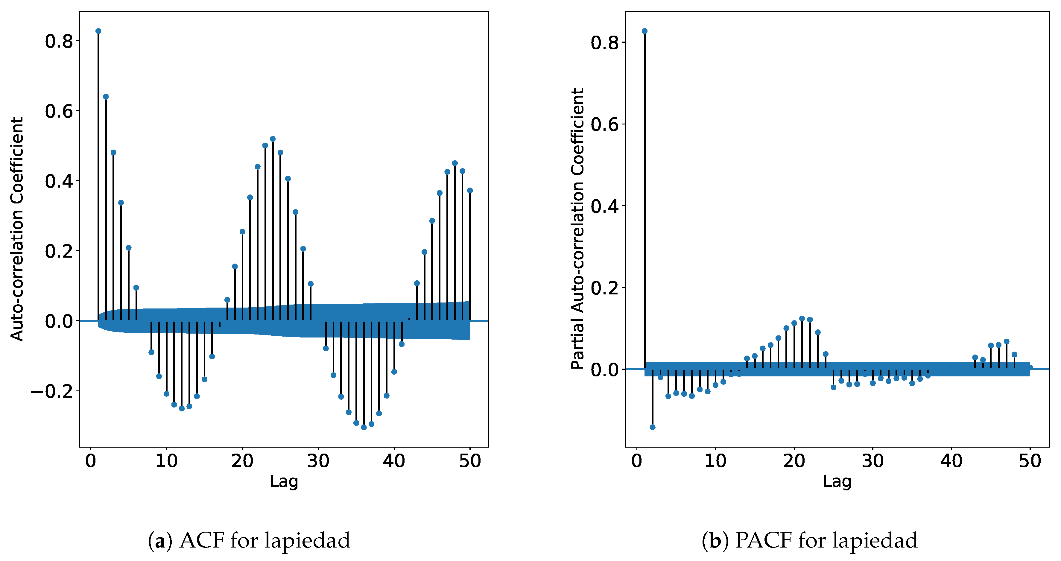
To identify periodicity in a time series it is necessary to analyze its auto-correlation plot. The Auto-Correlation Function (ACF) is the correlation of a signal (in this case a time series) with a delayed copy of itself. The ACF plot shows ACF as a function of delay.
Since some of the data sets are missing a few samples, it was necessary to identify the longest sequences without missing values, in order to calculate the dominant Lyapunov exponents. For brevity, only the auto-correlation and partial auto-correlation graphs for the time series 24908 and lapiedad are shown in
Figure 6 and
Figure 7, respectively.
In the plots, the x-axis represents the time lag, and the y-axis shows the auto-correlation coefficient and the partial auto-correlation coefficient for the ACF and PACF figures, respectively. The definitions of ACF and PACF are described in [
52]. In every plot there is an increased auto-correlation every 8 and 24 lags for the Russian and Michoacán stations, respectively. Many time lags exhibit auto-correlation values that exceed the 5% significance threshold; this fact indicates that the null hypothesis that there is no correlation for those time lags can be rejected.
4.2. Lyapunov Dominant Exponent Analysis of the Data Sets
Wind speed has been identified as a chaotic or as a non linear system [
58,
59,
60,
61]. To test these assertions we estimated the dominant Lyapunov exponents of the data sets used in this work.
To obtain the Lyapunov exponents we used an implementation of the algorithm described in [
62]. Although there exist different ways to estimate the exponents (such as the ones described in [
23,
63], or [
64]), we decided to use Rosenstein et al.’s implementation, since it is the more consistent in interpretation of the resulting exponent. Although it is desirable to use as much data as possible to obtain the exponents, only 1000 data points were used, in order to minimize the time consumed in this task. The Lyapunov exponents of the time series are shown in
Table 1, which includes the Lyapunov exponents of two time series, the Logistic Map [
65] and the Sine function. The table columns include the Time Series and the minimum, maximum, and average Lyapunov Exponents.
The calculated exponents are not as high as we expected, which indicates that wind speed is not dominated by noise. Those exponents indicates that the data contains predictable components (seen in part in their respective ACF), but they also explain the difficulty to predict this kind of data in the long term. The exponents obtained are consistent with the ones observed in the literature. In [
58] the MLE obtained for their data set is 0.115, while the average MLE obtained by all of the data sets used in this work is 0.116. The Lyapunov Exponents computed for both sets of wind time series provide a strong indication that the underlying process that produce the data are chaotic.
4.3. Experiments
An often required wind forecasting task is to forecast the wind speed for the following day. In order to gather more performance information than just one execution of the different forecasting algorithms, we perform a One Day Ahead forecast for the last 10 days of each time series. In performing One Day Ahead (ODA) forecasting, the forecaster generates the number of samples contained in one day of observations at a time.
After we have forecasted one whole day, we consider time advances and the next day of real wind speed observation is available. Since we are forecasting for 10 days, the last 10 days of measures of each data set were saved in the validation set; the rest of the data was used as training set. The sampling period of the Russian stations is three hours, while the sampling period of the Mexican stations is one hour. The number of samples used for training varied depending of the time series from 875 to 25,000 samples, while the length of the validation sets were 80 and 240 for the Russian and Mexican time series, respectively.
Experiment Settings
Each technique has different modelling considerations; those considerations are described in the following paragraphs, and the values used in the experiments are listed in
Table 2.
ARIMA—The ARIMA implementation we used was the one included in the R statistical package [
66]. The order of the ARIMA model was estimated using the
auto.arima function.
NN—To determine the NN parameters (
m,
, and
) we used the deterministic approach described by Kantz in [
23]. The deterministic approach uses the Mutual Information algorithm to obtain
and the False Nearest Neighbors algorithm to find an optimal
m;
is found by testing the number of neighbors found for an arbitrary
value, which is updated by the rule
when not enough neighbors are found.
NNDE—In NNDE the NN parameters are found by a DE optimization, where the evolutionary individuals are vectors of the form [m, , ]. Because of the stochastic nature of DE, this optimization process is executed 30 independent times. The set of parameters that yield the least error score is the one used to forecast.
FF—This technique compiles a set of fuzzy rules that describe the time series by using delay vectors of dimension
m and time delay
. These parameter values are set to the same as those obtained by the deterministic method used by NN [
23,
24]. Since the time series contains outliers, FF uses a simple filter which replaces any value greater than
(
is the standard deviation of the time series) with the missing value indicator.
ANN-cGA—This method determines the optimal topology of a MLP using Compact Genetic Algorithms. The optimization process consists in finding the optimal number of inputs (past observations), the number of hidden neurons, and the learning algorithm.
EvoDAG—EvoDAG uses its default parameters and m is set to three days behind.
Table 2 shows the parameters used by the techniques for ODA forecasting. With the exception of NNDE, all the forecasters use the same parameters. NNDE varies its parameters since the DE process can obtain different parameters depending of the forecasting scenario.
Once the different forecasting models were trained, we proceeded to test their forecasts for the proposed forecasting task.
4.4. Performance Analysis
For this comparison, 7 forecasters were used. Auto-Regressive Integrated Moving Average (ARIMA), and Nearest Neighbors (NN) are well known forecasting techniques in the time series area. Nearest Neighbors with Differential Evolution Optimization (NNDE), Fuzzy Forecasting (FF), Artificial Neural Network with Compact Genetic Algorithm Optimization (ANN-cGA), and EvoDAG are techniques proposed by the authors to tackle this forecasting problem.
As previously indicated, the Mexican Data Sets present missing values in both the training and validation sets. To preserve the integrity of the results, when forecasting, if the value to predict is a missing value that measure does not contribute to the error score of the forecaster.
To measure the performance of the forecasters, we used the Symmetric Mean Absolute Percentage Error (SMAPE).
SMAPE is defined in Equation (
7).
where
A are the actual values,
F are the forecasted values, and
n is the number of samples in both sets.
SMAPE was selected as error measure because it allows to compare the error between data sets, since it is expressed as a percentage. This can be also be done with the non-symmetric version of this error measure (Mean Average Percentage Error—MAPE). However, the data sets used contain many zero valued samples, which in MAPE lead to undetermined error values.
It is important to clarify that undetermined values can also occur with SMAPE. However, if there is a sum of zeros in the denominator, it indicates that the actual and forecasted values are zero, making the denominator and numerator of the fraction zero, which makes the contribution to the error meaningless.
4.5. One Day Ahead Forecasting
The One Day Ahead forecasting scenario represents the forecasting task this article is addressing. For this scenario each forecaster generates a day of estimations at a time. Once these forecasts are made, one day of observations are taken from the validation set and are incorporated into the training set (replacing the values introduced by the forecaster), and the process is repeated until 10 days of forecasts are completed.
Table 3 shows the SMAPE scores of the 10 day forecasts produced by the different forecasting techniques.
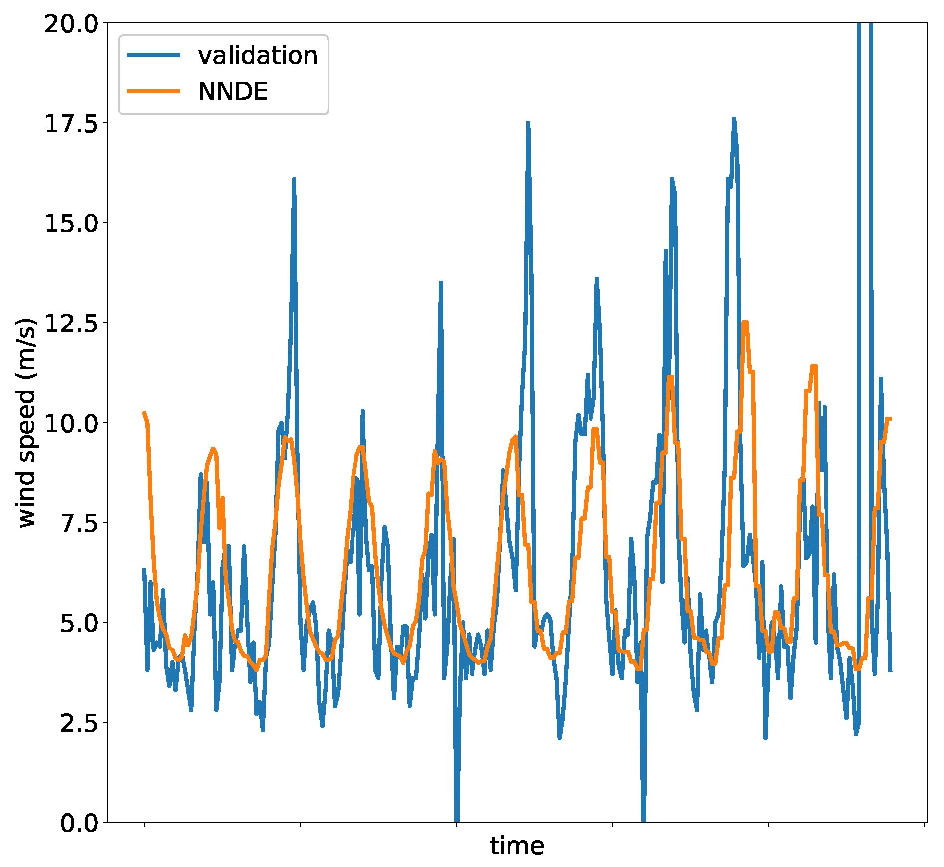
NNDE produces the best scores in most stations, which indicates that, for these time series, it is well suited to forecast many samples in advance, compared to the other forecasters (at least for this particular forecasting task).
Figure 8 presents a plot of the forecast of the winning model, NNDE, for the malpais time series. As discussed earlier in the article, the quality of the data is not as one could expect. Time Series contain noise, outliers, and missing data, not to count the fact that they are chaotic. Those characteristics make them extremely difficult to forecast. Nonetheless, from the figure, we can observe that the model closely predicts the cyclic behavior of the data, not being able to account for the noise included in the validation set, nor the outliers.
Section 2 includes a discussion on Okumus et al.’s survey article, which provides errors obtained in several works in the area. Those errors are reported for different forecasting tasks, using different error metrics, so we cannot objectively compare the performance of the methods we present in this article with those presented in the articles included in the survey.
5. Conclusions
A set of forecasting methods based on Soft Computing and the comparison of their performances, using a set of wind speed time series available to the public, has been presented. The set of methods used in the performance comparison are Nearest Neighbors (the original method, and a version where its parameters are tuned by Differential Evolution—NNDE), Fuzzy Forecasting, Artificial Neural Networks (designed and tuned by Compact Genetic Algorithms), and Genetic Programming (EvoDAG). For the sake of comparison, we have included ARIMA (a non AI-based method).
The experiments were carried out using twenty time series with wind speed, ten of them correspond to Russian weather stations and the other ten come from Mexican weather stations. The Russian time series are sampled at intervals of 8 h and expressed as integers, while the Mexican time series were sampled at intervals of one hour, using one decimal digit. The maximum exponents of Lyapunov were calculated for each time series’, which show that the time series are chaotic. In summary, the data we use for comparison are chaotic, contain noise, and have many missing values, therefore, these time series are difficult to predict in the long term.
The forecasting task was to predict one day ahead, repeated for 10 days. This forecasting task represents 80 measurements for the Russian and 240 for the Mexican time series.
In addition to comparing the performance of forecasting techniques, the use of phase space reconstruction to determine the important contributions of the past as input to forecasting models was presented. Two parameters from the reconstruction process can be used in time series forecasting methods: m (the embeding dimension) and (the time delay or sub-sampling constant). These parameters provide an insight into what part of the history of the time series can be used in the regression process. Nevertheless, most of the work on forecasting using ANN, just considers some window in the past of the history, normally given by the experience of experts in the application field, and no sub-sampling is used at all. Other statistical methods provide information about what part of the history of the time series is of importance in the forecasting process. For instance, ARIMA frequently uses the information provided by the ACF and PACF functions.
The results of the performance comparison show that NNDE outperforms the other methods in a vast majority of cases for OSA forecasting and in more than half in ODA forecasting. It is well known that the results of a performance comparison depend heavily on the error criterion used to measure the performance of the forecasting techniques. In this case, we used MSE and SMAPE; NNDE won under both error functions, which places this technique as the most suitable for the forecasting tasks used in this comparison.
We expect the results of this study to be useful for the renewable energy and time series forecasting scientific communities.

 ,
, 


