Least Squares Support Vector Mechanics to Predict the Stability Number of Rubble-Mound Breakwaters


Civil Engineering Department, Faculty of Engineering, Balikesir University, 10145 Balikesir, Turkey
Water 2018, 10(10), 1452; https://doi.org/10.3390/w10101452
Submission received: 31 August 2018
/
Revised: 11 October 2018
/
Accepted: 11 October 2018
/
Published: 15 October 2018
(This article belongs to the Special Issue Machine Learning Applied to Hydraulic and Hydrological Modelling)
Abstract
:In coastal engineering, empirical formulas grounded on experimental works regarding the stability of breakwaters have been developed. In recent years, soft computing tools such as artificial neural networks and fuzzy models have started to be employed to diminish the time and cost spent in these mentioned experimental works. To predict the stability number of rubble-mound breakwaters, the least squares version of support vector machines (LSSVM) method is used because it can be assessed as an alternative one to diverse soft computing techniques. The LSSVM models have been operated through the selected seven parameters, which are determined by Mallows’ Cp approach, that are, namely, breakwater permeability, damage level, wave number, slope angle, water depth, significant wave heights in front of the structure, and peak wave period. The performances of the LSSVM models have shown superior accuracy (correlation coefficients (CC) of 0.997) than that of artificial neural networks (ANN), fuzzy logic (FL), and genetic programming (GP), that are all implemented in the related literature. As a result, it is thought that this study will provide a practical way for readers to estimate the stability number of rubble-mound breakwaters with more accuracy.
1. Introduction
One of the most essential structural coastal protection methods is the usage of breakwaters. These structures are implemented to protect coastal areas and to prevent siltation in river mouths. It also provides security against the waves coming offshore, while at the same time it ensures protection for marine vessels entering the port. Essentially these structures are designed to absorb the available coastal energy. Rubble-mound breakwaters are one of the most frequently used breakwater kinds over the world. These breakwaters consist of three layers; filter, core, and armor layer. The most crucial parameter in the design of the breakwater is to obtain data about the stability number of armor blocks. In the literature, empirical formulas of Hudson [1] and Van der Meer [2] have been suggested, using experimental studies in the context of stability analyses for rubble-mound breakwaters. Kaku [3], Smith et al. [4], and Hanzawa et al. [5] have put forward new empirical equations with reference to Van der Meer’s experimental data. However, these equations are not enough to diminish uncertainties originated from the process. Recently, soft computing tools such as artificial neural networks (ANN), support vector machine (SVM), and adaptive neuro-fuzzy inference system (ANFIS) have started to be employed both to cope with several troubles and to minimize the time and cost spent on experimental works. Mase et al. [6] and Kim and Park [7] reported that the ANN technique yielded better results than those of empirical model-based approaches in the breakwater design. Yagci et al. [8] used three different types of ANN and fuzzy based techniques to determine the damage rates of the breakwater. According to their evaluations, it has been deduced that all methods produce results which are quite close to the experimental values. Despite the many advantages of ANN-derived methods, there are some disadvantages as well. Some of them are different complexity in the structure of the multi-layer structure, trapping in local minimums, possibility of over-training, difficulty in sensitivity analysis of parameters, and random output of assigned weights so that different outputs are generated in each run of the network [9]. To depress the drawbacks of ANN, Vapnik [10] developed a support vector machines (SVM) method based upon machine learning theory and solutions with quadratic programming. While this technique maintains all the strengths of the ANN, it shows up to be a robust alternative to make out some of the prominent weaknesses associated with ANN [11]. SVM methods have been exported to various fields of water engineering, such as hydrology and coastal researches, and significant inferences have been put forward [12,13,14,15,16]. An exemplary application of SVM is presented by Kim et al. [17] under the estimation of stability numbers of rubble-mound breakwaters. From their work, predictions derived from support vector regression (SVR) have been compared with those of the empirical equation and ANN. As result of comparisons that has been conducted in their study, the superiority of SVM has been emphasized. In the literature, this method is also applied to the areas of coastal engineering, such as prediction of wave transmission over a submerged reef [18], damage level prediction of non-reshaped berm breakwater [19,20,21], and wave transmission of floating pipe breakwater [22].
Most of the soft computing models mentioned above are based upon Van der Meer data as training data and at this stage, generally a trial and error method has been employed for predictor selection. Table 1 summarizes the input sets recommended by different researchers. Here, P is permeability of breakwater, Nw is the number of waves, S is damage level, εm is surf similarity parameter, cotθ is slope angle, h is water depth, h/Hs dimensionless water depth, SS is spectral shape, Ls is the period of significant wave, Hs significant wave heights in front of the structure, and Ts is wave period [7]. If it is regarded that there are 2N-1 input combination under N inputs defined, it will not be credible to figure out the predictor extraction by means of a basic approach like trial and error. In the presented study, the predictor selection process was automated by Mallows’ Cp approach. Using this approach, the best possible subsets within different inputs have been determined and then presented as inputs to the least squares version of the support vector machine (LSSVM). The particle swarm optimization (PSO) is implemented in the LSSVM calibration step to ensure that the trained model offers a global solution without being encountered to the local minimum. It is thought that the modeling strategy that includes the above process steps has novelty and at the same time it can ensure a practical solution for the research pertaining to the topic indicated in the title of this paper.
2. Prevalent Formulas for Prediction of Stability Number
Stability number of rubble-mound breakwaters in reference to wave attack is defined as:
where Hs is the significant wave height, ∆ is relative mass density, and Dn50 is the nominal diameter of armor unit. To estimate the stability number, Hudson [1] proposed an empirical formula:
where KD is stability coefficient (depends upon the form of the armor unit, method of placement, and so on). Considering other parameters that are not considered in Equation (2), Van deer Meer [2] has improved two stability formulas for both surging and plunging waves as follows:
where εm is surf similarity parameter () dependent on the average wave period Tm, εc is the critical surf similarity parameter () describing the transition from plunging to surging waves.
By using H50 instead of Hs in Van Der Meer formulas (Equations (3a) and (3b)), Vidal et al. [27] obtained the following equations. H50 is the average wave height of the 50 highest waves hitting a rubble-mound breakwater.
where N50 is defined as ().
3. Methods and Data
3.1. Least Squares Support Vector Machines
Support vector machines (SVM) applied as regression is a soft computing tool developed within a statistical learning theory by concerning various error optimization stages [22,28]. Despite the prosperous performance of standard SVM, it has some shortcomings. Some of them are (i) that SVM employs basis functions superfluously in that the needed support vectors increase with the training data size, (ii) there is a dubiousness to get the control parameters. Thus, the calibration of the three parameters of SVM can be time-consuming and wearing.
On the other hand, the LSSVMs supply a computational benefit over standard SVM by transforming quadratic optimization issues to the linear equation system [29].
Given a training set for a regression application, where is the input vector, is the related output, and N is the data point number, the aim of LSSVM is to get . In LSSVM, the minimization of the cost-function is defined as:
Subjected to the constraint
where is the weight, is the quadratic loss component, and C is a parameter used as regularization [14,16]. The solution of this optimization problem originated from LSSVM’s structure and can be attained by using the Lagrange multipliers as follows:
where are Lagrange multipliers. The conditions regarding the optimal solution can be generated by taking first-order partial derivatives of Equation (7) with respect to and , respectively, and then equaling the system of equations to zero values such that:
The solution of the constrained optimization problem pertaining to LSSVM modeling including Lagrange multipliers gives values such that:
where is the Lagrange multiplier, which is obtained by referencing Equation (7) [30]. The LSSVM function output can be obtained as follows:
where for is the kernel function and is the bias term. Any kernel function can be preferred in accordance with Mercer’s theorem [31,32,33].
3.2. Kernel Function
The kernel functions treated by LSSVM modeling studies are generally some specific functions including linear, spline, polynomial, sigmoid, and Gaussian radial basis [32,33,34,35,36,37]. In previous studies existing in the literature, the Gaussian radial basis function (RBF) was chosen as the kernel function because it can map samples nonlinearly into a higher dimensional space and is able to tackle the situation having nonlinearity [38].
where σ is the width of function, at the same time, a control parameter of LSSVM.
Keerthi et al. [39] revealed that the linear type showed similar performance with the RBF kernel function. Lin and Lin [40] proved that the sigmoid type had similar performances with RBF. Additionally, Lin et al. [35] have pointed out that the RBF kernel is less numerical complex in comparison with polynomial type since it requires many more hyper-parameters than those of the RBF version.
3.3. Optimization Algorithm Used in LSSVM Calibration: PSO
In the modeling stage of LSSVM that have C and σ parameters to be tuned, the PSO algorithm, which is a population-based heuristic algorithm brought forward by Kennedy and Eberhart [41], inspired by the social behavior of birds, was preferred. LSSVM is calibrated by the grid search approach standard [13,14,15]. Because PSO is a successful algorithm in terms of global search capability, extra attention has been given to more precise training of LSSVM. Implementation of LSSVM combined with PSO for another concept has been given by Hu et al. [42]. The readers can reach this study to get more details about the procedure.
In PSO, for each particle that is initially randomized, the local best (pbest) is found in each generation (or iteration). The number of pbest in the swarm is equal to the number of particles. After enough iterations, the global best (gbest) solution is determined from the local solutions by means of velocities and position update operators. The detailed information and the related formulas about this algorithm have been given by Okkan et al. [43].
3.4. Data Sets
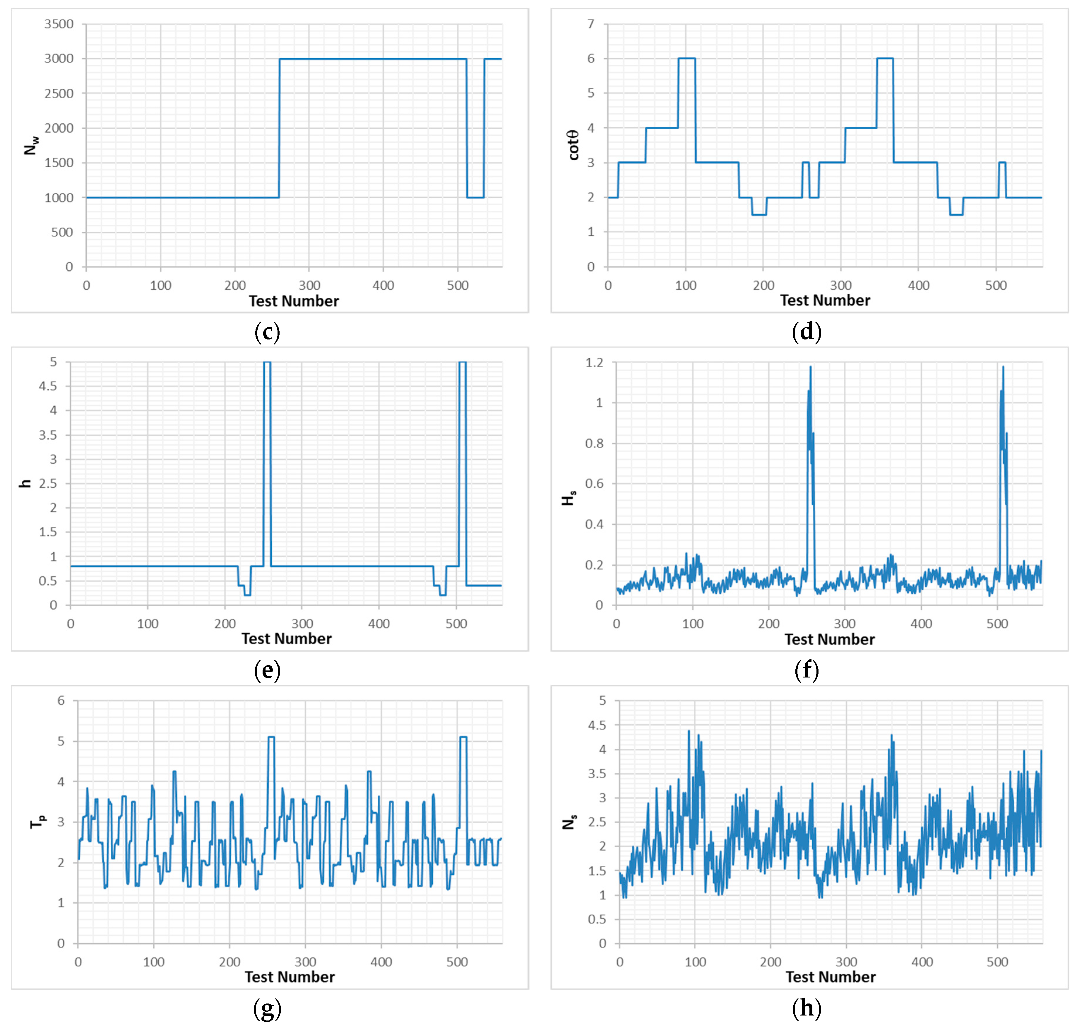
Input and output data must be specified to apply LSSVM in the phase of predicting the stability numbers. Van Der Meer’s [44] 558 data sets regarding low-crest, large scale, and small scale were used for the training model, while 85 data sets were used to validate the performance of the trained LSSVM model. There are seven parameters that make up input vectors for the model. Here, P is permeability of breakwater, S is damage level, Nw is the number of waves, cotθ is slope angle, h is water depth, Hs is significant wave heights in front of the structure, Tp is peak wave period, and Ns (stability number) is output data to be predicted. The ranges of variables of randomly selected training and testing data sets are given in Table 2. Additionally, the data of seven parameters used in the training test are presented in Figure 1.
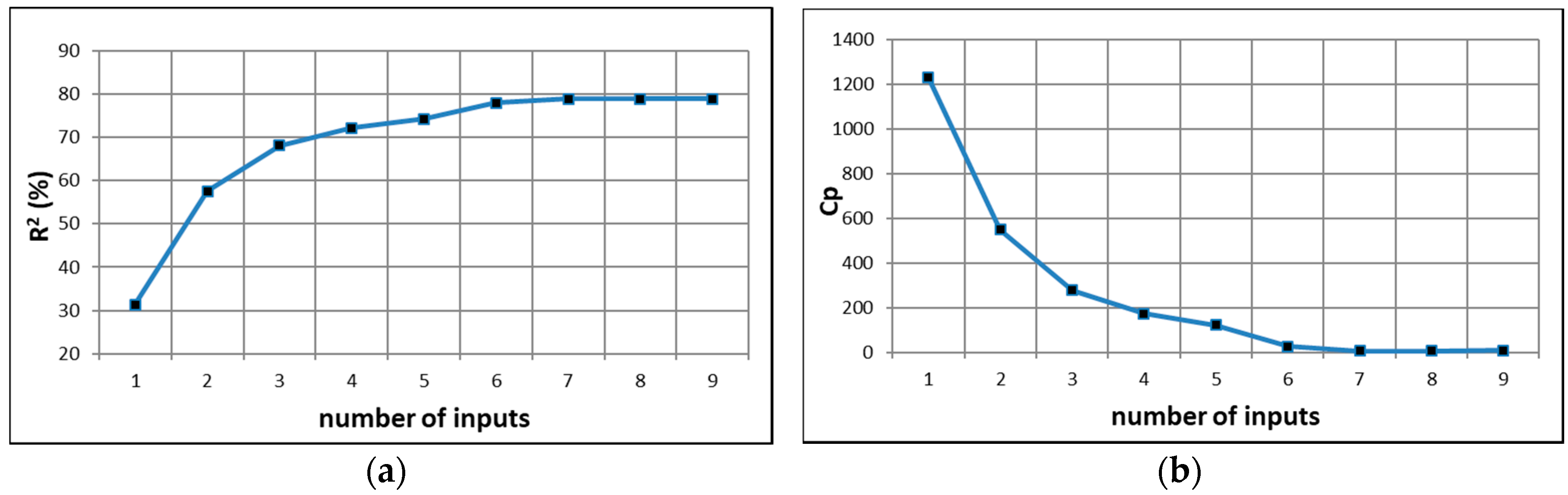
The statistics obtained in Table 3 are re-emphasized in Figure 2. It is apparent that there is no relative difference between the linear model with seven inputs and the full linear model with nine inputs. The lowest calculated Cp coefficient, 6.6, also proves this view. Thus, the uncertainty in the input determination stage and the decision-making process has been moderated. These inputs are then intended to be input to the LSSVM model to improve predictions.
The elementary predictors specified in the previous section have been prepared to be supplied as inputs to the LSSVM model. Five hundred and fifty-eight data points used in the predictor selection phase were also evaluated in model training, while 85 data points were used in validation of the calibrated model. Since it is known that the data set has extreme values, all input and target values should be normalized before training in order not to affect the generalization ability of the model adversely. The results were compared using two different normalization techniques given in Equations (12) and (13), respectively, in the study content.
where is the scaled normalized value, is the data, and are, respectively, the minimum and maximum values of the data, and and S are, respectively, the mean and unbiased standard deviation statistics of the data [37].
4. Results
In the study, the LSSVM models in which the aforesaid normalization techniques were applied were named as LSSVM (model 1) and LSSVM (model 2), respectively. In the training of models, the PSO algorithm was used. The study was carried out on a MATLAB code [14].
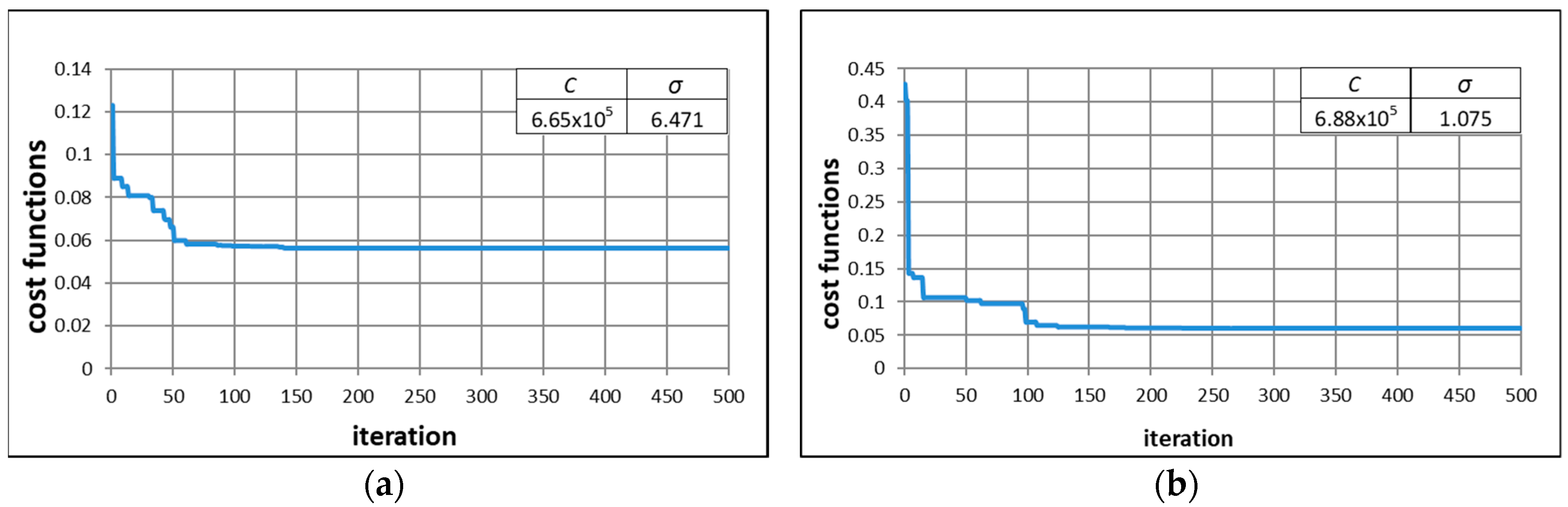
Here, the acceleration coefficients of the PSO were fixed and taken as 2. In addition, minimum and maximum inertia weights controlling the algorithm were assigned 0.4 and 0.9, respectively. In the pool of population to be employed in the generations, it was considered enough to use 20 particles while Lagrangian multipliers, and hence the weights of the LSSVM models, exposed to 500 iterations were calibrated during the training data, the performance of the testing was taken as the most suitable C and σ estimations. The situation of the root meansquare error (RMSE) used as a cost value throughout the implemented generations and the determined LSSVM parameters are shown in Figure 3.
After estimating the LSSVM control parameters, the training and test results produced by the models were examined. The summary of the evaluation in terms of R2 and RMSE statistics is given in Table 4.
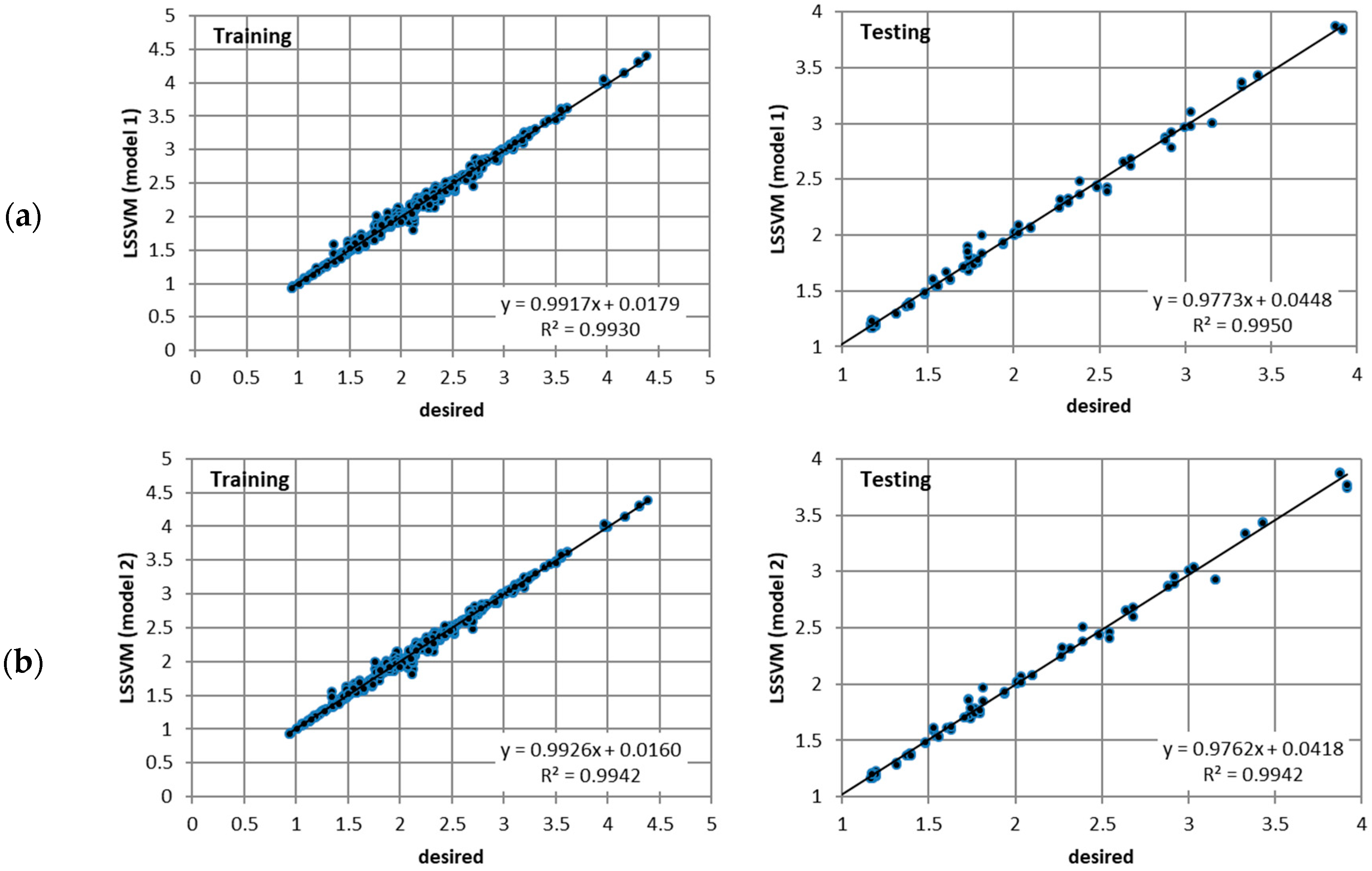
Under two different normalization techniques, the LSSVM models showed similar responses during both the training and testing stages. However, it can be discussed that first normalization is clearly more successful in the testing phases. The first model showed a 0.08% increase in R2 and 7% less RMSE compared to the second model. It can be understood from the scatter diagrams given in Figure 4 that the first model is more favorable in terms of systematic biases over the fitted lines. In summary, the precise result of the LSSVM (model 1) is noteworthy. To examine success of the proposed LSSVM models on stability number prediction, a conventional technique termed as multiple linear regression model (MLRM) was also used. MLRM analysis is performed by MS-Excel software. MLRM model having seven parameters and one interception was constructed from the same training set of LSSVM. Then, computed MLRM coefficients were quarried over the testing set as well. The last column of Table 4 includes MLRM performances in point of both RMSE and R2. From Table 4 again, the weak results of MLRM have proved that it cannot overcome the nonlinearities originated from data distributions and the LSSVM typed model must be appealed for this mentioned issue.
Moreover, the correlation coefficients of the different soft computing methods are summarized in Table 5. As can be seen from Table 5, the established model enhanced the best correlation coefficient founded in the literature by 1.5%. This argument turns out that the LSSVM method is apparently better than other soft computing methods.
5. Conclusions
In the literature, there are suggested empirical formulas generated from experimental studies to determine the number of stabilities in the protection layer of breakwaters, one of the structural coastal protection methods. In the last decade, soft computing tools have been used not only to reduce these uncertainties that come from the formulas, but to minimize the time and cost in the experimental works. In this study, the LSSVM method, which maintains the strengths of ANN and overcomes some deficiencies, is used so as to estimate the number of stabilities of rubble-mound breakwaters based on Van Der Meer’s [44] laboratory data. Seven input data were determined by using Mallows’ Cp approach, which determines the best possible predictors among the great deal of different inputs. These are permeability of breakwater, damage level, the number of waves, slope angle, water depth, significant wave heights in front of the structure, and peak wave period. Two different normalization techniques in the LSSVM models are applied. In the training of models, the PSO algorithm is operated by means of a MATLAB code. It can be seen that first normalization is clearly more successful in the testing phases. The performance of the LSSVM models was found to be of a higher accuracy (correlation coefficients (CC) of 0.997) and better than other soft computing methods, as shown in Table 5. It is thought that the results of this study are quite successful compared to the results attributed to the literature and would be an inspirational example for other researchers.
Despite various advantages of LSSVM calibrated through PSO, the estimations of control parameters, which are C and σ, respectively, may have taken place in a vast solution space with two dimensions. Especially, C parameters has shown rather extreme values (i.e., 6.65 × 10⁵, 6.88 × 10⁵ for LSSVM model 1 and 2, respectively). Even if the PSO has set out stable behavior in the finding of global minimums, determining the optimal estimations of LSSVM parameters have such an uneasy process as it challenges the computer capacity. In this context, one-parameter version of support vector machines, namely relevance vector machines (RVM) can be a more robust alternative in terms of training and setting a nonlinear regression architecture. In the hydraulic literature, RVM has shown a superior response compared to that of counterparts (for example, References [12,33,36,37]). The issues regarding the implementation of RVM to the same problems in this study will be the future direction.
Funding
This research received no external funding.
Conflicts of Interest
The author declares no conflict of interest.
References
- Hudson, R.Y. Design of Quarry Stone Cover Layer for Rubble Mound Breakwaters; U.S. Army Engineer Research Report No. 2-2; Waterways Experiment Station, Coastal Engineering Research Centre: Vicksburg, MS, USA, 1958. [Google Scholar]
- Van Der Meer, J.W. Deterministic and probabilistic design of breakwater armor layers. J. Wtrwy. Port Coast. Ocean Eng. 1988, 114, 66–80. [Google Scholar] [CrossRef]
- Kaku, S. Hydraulic Stability of Rock Slopes Under Irregular Wave Attack. Master’s Thesis, University of Delaware, Newark, DE, USA, 1990. [Google Scholar]
- Smith, W.G.; Kobayashi, N.; Kaku, S. Profile Changes of Rock Slopes by Irregular Waves. In Proceedings of the 23th International Conference Coast Engineering ASCE, New York, NY, USA, 4–9 October 1992; pp. 1559–1572. [Google Scholar]
- Hanzawa, M.; Sato, H.; Takahashi, S.; Shimosako, K.; Takayama, T.; Tanimoto, K. New Stability Formula for Wave-Dissipating Concrete Blocks Covering Horizontally Composite Breakwaters. In Proceedings of the 25th Coastal Engineering Conference, ASCE, Orlando, FL, USA, 2–6 September 1996; pp. 1665–1678. [Google Scholar]
- Mase, H.; Sakamoto, M.; Sakai, T. Neural network for stability analysis of rubble-mound breakwaters. J. Wtrwy. Port Coast. Ocean Eng. 1995, 121, 294–299. [Google Scholar] [CrossRef]
- Kim, D.H.; Park, W.S. Neural network for design and reliability analysis of rubble mound breakwaters. Ocean Eng. 2005, 32, 1332–1349. [Google Scholar] [CrossRef]
- Yagci, O.; Mercan, D.E.; Cigizoglu, H.K.; Kabdasli, M.S. Artificial intelligence methods in breakwater damage ratio estimation. J. Ocean Eng. 2005, 32, 2088–2106. [Google Scholar] [CrossRef]
- ASCE Task Committee. Artificial neural networks in hydrology—I: Preliminary concepts. J. Hydrol. Eng. 2000, 5, 115–123. [Google Scholar] [CrossRef]
- Vapnik, V.N. The Nature of Statistical Learning Theory; Springer: Berlin/Verlag, Germany, 1995; ISBN 0-387-94559-8. [Google Scholar]
- ASCE Task Committee. Artificial neural networks in hydrology—II: Hydrological applications. Hydrol. Eng. 2000, 5, 124–137. [Google Scholar] [CrossRef]
- Samui, P.; Dixon, B. Application of support vector machine and relevance vector machine to determine evaporative losses in reservoirs. Hydrol. Process. 2012, 26, 1361–1369. [Google Scholar] [CrossRef]
- Suykens, J.A.K.; Vandewalle, J. Least squares support vector machine classifiers. Neural Process. Lett. 1999, 9, 293–300. [Google Scholar] [CrossRef]
- Suykens, J.A.K.; Van Gestel, T.; De Brabanter, J.; De Moor, B.; Vandewalle, J. Least Squares Support Vector Machines; World Science: Singapore, 2002. [Google Scholar] [CrossRef]
- Van Gestel, T.; Suykens, J.A.K.; Baesens, B.; Viaene, S.; Vanthienen, J.; Dedene, G.; De Moor, B.; Vandewalle, J. Benchmarking least squares support vector machine classifiers. Mach. Learn. 2004, 54, 5–32. [Google Scholar] [CrossRef]
- Okkan, U.; Serbes, Z.A. Rainfall-runoff modelling using least squares support vector machines. Environmetrics 2012, 23, 549–564. [Google Scholar] [CrossRef]
- Kim, D.; Kim, D.H.; Chang, S.; Lee, J.J.; Lee, D.H. Stability number prediction for breakwater armor blocks using support vector regression. KSCE J. Civ. Eng. 2011, 15, 225–230. [Google Scholar] [CrossRef]
- Kuntoji, G.; Rao, M.; Rao, S. Prediction of wave transmission over submerged reef of tandem breakwater using PSO-SVM and PSO-ANN techniques. ISH J. Hydraul. Eng. 2018. [Google Scholar] [CrossRef]
- Sukomal, M.; Rao, S.; Harish, N. Damage level prediction of non-reshaped berm breakwater using ANN, SVM and ANFIS models. Int. J. Nav. Arch. Ocean 2012, 4, 112–122. [Google Scholar] [CrossRef]
- Harish, N.; Mandal, S.; Rao, S.; Patil, S.G. Particle swarm optimization based support vector machine fordamage level prediction of non-reshaped berm breakwater. Appl. Soft. Comput. 2015, 27, 313–321. [Google Scholar] [CrossRef]
- Kuntoji, G.; Rao, S.; Mandal, S. Application of support vector machine technique for damage level prediction of tandem breakwater. Int. J. Earth Sci. Eng. 2017, 10, 633–638. [Google Scholar] [CrossRef]
- Patil, S.G.; Mandal, S.; Hegde, A.V. Genetic algorithm based support vector machine regression in predicting wave transmission of horizontally interlaced multi-layer moored floating pipe breakwater. Adv. Eng. Softw. 2012, 45, 203–212. [Google Scholar] [CrossRef]
- Balas, C.E.; Koç, M.L.; Tür, R. Artificial neural networks based on principal component analysis, fuzzy systems and fuzzy neural networks for preliminary design of rubble mound breakwaters. Appl. Ocean Res. 2010, 32, 425–433. [Google Scholar] [CrossRef]
- Erdik, T. Fuzzy logic approach to conventional rubble mound structures design. Expert Syst. Appl. 2009, 36, 4162–4170. [Google Scholar] [CrossRef]
- Shahidi, A.E.; Bonakdar, L. Design of rubble-mound breakwaters using M50 machine learning method. Appl. Ocean Res. 2009, 31, 197–201. [Google Scholar] [CrossRef]
- Koç, M.L.; Balas, C.E.; Koç, D.İ. Stability assessment of rubble-mound breakwaters using genetic programming. Ocean Eng. 2016, 111, 8–12. [Google Scholar] [CrossRef]
- Vidal, C.; Medina, R.; Lomonanco, P. Wave height parameter for damage description of rubble mound breakwater. Coast. Eng. 2006, 53, 712–722. [Google Scholar] [CrossRef]
- Vapnik, V. Statistical Learning Theory; John Wiley & Sons: Toronto, ON, Canada, 1998. [Google Scholar]
- Suykens, J.A.K. Nonlinear Modelling and Support Vector Machines. In Proceedings of the 18th IEEE Instrumentation and Measurement Technology Conference, Budapest, Hungary, 21–23 May 2001. [Google Scholar]
- Ekici, B.B. A least squares support vector machine model for prediction of the next day solar insolation for effective use of PV systems. Measurement 2014, 50, 255–262. [Google Scholar] [CrossRef]
- Mercer, J. Functions of positive and negative type and their connection with the theory of integral equations. Philos. Trans. R. Soc. 1909, 209, 415–446. [Google Scholar] [CrossRef]
- Okkan, U.; Inan, G. Statistical downscaling of monthly reservoir inflows for Kemer watershed in Turkey: Use of machine learning methods, multiple GCMs and emission scenarios. Int. J. Climatol. 2015, 35, 3274–3295. [Google Scholar] [CrossRef]
- Okkan, U.; Serbes, Z.A.; Samui, P. Relevance vector machines approach for long-term flow prediction. Neural Comput. Appl. 2014, 25, 1393–1405. [Google Scholar] [CrossRef]
- Liong, S.Y.; Sivapragasam, C. Flood stage forecasting with support vector machines. J. Am. Water Resour. Assoc. 2002, 38, 173–186. [Google Scholar] [CrossRef]
- Lin, J.Y.; Cheng, C.T.; Chau, K.W. Using support vector machines for long-term discharge prediction. Hydrol. Sci. J. 2006, 51, 599–612. [Google Scholar] [CrossRef] [Green Version]
- Ghosh, S.; Mujumdar, P.P. Statistical downscaling of GCM simulations to streamflow using relevance vector machine. Adv. Water Resour. 2008, 31, 132–146. [Google Scholar] [CrossRef]
- Okkan, U.; Inan, G. Bayesian learning and relevance vector machines approach for downscaling of monthly precipitation. J. Hydrol. Eng. 2015, 20, 04014051. [Google Scholar] [CrossRef]
- Aich, U.; Banerjee, S. Modeling of EDM responses by support vector machine regression with parameters selected by particle swarm optimization. Appl. Math. Model. 2014, 38, 2800–2818. [Google Scholar] [CrossRef]
- Keerthi, S.S.; Shevade, S.K.; Bhattacharyya, C.; Murthy, K.R.K. Improvements to Platt’s SMO algorithm for SVM classfier design. Neural Comput. 2001, 13, 637–649. [Google Scholar] [CrossRef]
- Lin, H.T.; Lin, C.J. A Study on Sigmoid Kernels for SVM and the Training of Non-PSD Kernels by SMO-Type Methods; Technical Report; Department of Computer Science and Information Engineering, National Taiwan University: Taipei, Taiwan, 2003; Available online: http://www.work.caltech.edu/htlin/publication/doc/tanh.pdf (accessed on 2 August 2018).
- Kennedy, J.; Eberhart, R.C. Particle Swarm Optimization. In Proceedings of the IEEE International Conference on Neural Networks, Perth, WA, Australia, 27 November–1 December 1995; IEEE Service Center: Piscataway, NJ, USA; pp. 1942–1948. [Google Scholar] [CrossRef]
- Hu, D.; Mao, W.; Zhao, J.; Guirong, Y. Application of LSSVM-PSO to Load Identification in Frequency Domain. In Proceedings of the International Conference on Artificial Intelligence and Computational Intelligence, AICI, Shanghai, China, 7–8 November 2009; pp. 231–240. [Google Scholar]
- Okkan, U.; Gedik, N.; Uysal, H. Usage of differential evolution algorithm in the calibration of parametric rainfall-runoff modeling. In Handbook of Research on Predictive Modeling and Optimization Methods in Science and Engineering; Kim, D., Roy, S.S., Länsivaara, T., Deo, D., Samui, P., Eds.; IGI Global: Hershey, PA, USA, 2018; pp. 481–499. [Google Scholar] [CrossRef]
- Van Der Meer, J.W. Rock Slopes and Gravel Beaches under Wave Attack; No. 396; Delft Hydraulics Publication: Delft, The Netherlands, 1988. [Google Scholar]
Figure 1.
Seven parameters used in the training test: (a) permeability of breakwater; (b) damage level; (c) the number of waves; (d) slope angle; (e) water depth; (f) significant wave heights; (g) peak wave period; (h) stability parameter that is modeled by variables denoted between (a,g).
Figure 1.
Seven parameters used in the training test: (a) permeability of breakwater; (b) damage level; (c) the number of waves; (d) slope angle; (e) water depth; (f) significant wave heights; (g) peak wave period; (h) stability parameter that is modeled by variables denoted between (a,g).


Figure 2.
Graphical display of produced (a) R2; (b) Cp for combinations determined by Mallows’ Cp under different input numbers.
Figure 2.
Graphical display of produced (a) R2; (b) Cp for combinations determined by Mallows’ Cp under different input numbers.

Figure 3.
Cost functions pertaining to (a) least squares version of support vector machines (LSSVM) (model 1) and (b) LSSVM (model 2) during generations.
Figure 3.
Cost functions pertaining to (a) least squares version of support vector machines (LSSVM) (model 1) and (b) LSSVM (model 2) during generations.

Figure 4.
Distributions of outputs produced by (a) LSSVM (model 1); (b) LSSVM (model 2) against desired values for both training and testing processes.
Figure 4.
Distributions of outputs produced by (a) LSSVM (model 1); (b) LSSVM (model 2) against desired values for both training and testing processes.


Table 1.
The input sets recommended by different researchers using the soft computing models.
| Methods | Author(s) | INPUT DATA | |||||||||||
|---|---|---|---|---|---|---|---|---|---|---|---|---|---|
| P | Nw | S | εm | Cotθ | h/Hs | SS | h/Ls | Hs | Hs/Ls | Ts | |||
| ANN | Mase et al. [6] | ● | ● | ● | ● | ● | ● | ||||||
| Kim and Park [7] | I | ● | ● | ● | ● | ● | ● | ||||||
| II | ● | ● | ● | ● | ● | ||||||||
| III | ● | ● | ● | ● | ● | ● | |||||||
| IV | ● | ● | ● | ● | ● | ● | ● | ||||||
| V | ● | ● | ● | ● | ● | ● | ● | ● | |||||
| Balas et al. [23] | I | ● | ● | ● | ● | ● | |||||||
| II | ● | ● | ● | ● | |||||||||
| FL | Erdik [24] | ● | ● | ● | ● | ● | ● | ||||||
| MT (Model Trees) | Shadidi and Bonakdar [25] | I | ● | ● | ● | ● | ● | ||||||
| II | ● | ● | ● | ● | ● | ● | |||||||
| SVR | Kim et al. [17] | ● | ● | ● | ● | ● | ● | ||||||
| GP | Koc et al. [26] | ● | ● | ● | ● | ● | |||||||
Table 2.
The range of variables in the training and testing data sets.
| Data Feature | Variables | Training Data (558 data Points) | Testing Data (85 Data Points) |
|---|---|---|---|
| Input | P | 0.1–0.6 | 0.1–0.6 |
| S | 0.32–46.38 | 0.35–45.86 | |
| Nw | 1000–3000 | 1000–3000 | |
| cotθ | 1.5–6 | 1.5–6 | |
| h | 0.2–5 | 0.4–5 | |
| Hs | 0.0461–1.18 | 0.0461–1.07 | |
| Tp | 1.33–5.1 | 1.33–5.1 | |
| Output | Ns | 0.94–4.38 | 0.79–3.91 |
Table 3.
The optimal regression models with i inputs obtained from the Mallows Cp approach.
| Number of Inputs | R2 | Cp | P | S | Nw | ξm | cotθ | Tm | Tp | Hs | h |
|---|---|---|---|---|---|---|---|---|---|---|---|
| 1 | 31.3 | 1229.7 | ● | ||||||||
| 2 | 57.6 | 548.8 | ● | ● | |||||||
| 3 | 68.1 | 278.3 | ● | ● | ● | ||||||
| 4 | 72.2 | 173.5 | ● | ● | ● | ● | |||||
| 5 | 74.2 | 123.4 | ● | ● | ● | ● | ● | ||||
| 6 | 78 | 26.4 | ● | ● | ● | ● | ● | ● | |||
| 7* | 78.9 | 6.6 | ● | ● | ● | ● | ● | ● | ● | ||
| 8 | 78.9 | 8.2 | ● | ● | ● | ● | ● | ● | ● | ● | |
| 9 | 78.9 | 10 | ● | ● | ● | ● | ● | ● | ● | ● | ● |
* Bold values in Table 3 show proper results regarding Cp coefficient.
Table 4.
Statistical performances of least squares version of support vector machines (LSSVM) models and multiple linear regression model (MLRM) in training and testing phases.
Table 4.
Statistical performances of least squares version of support vector machines (LSSVM) models and multiple linear regression model (MLRM) in training and testing phases.
| Data Portion | LSSVM (Model 1) | LSSVM (Model 2) | MLRM | |||
|---|---|---|---|---|---|---|
| RMSE | R2 | RMSE | R2 | RMSE | R2 | |
| Training | 0.0531 | 0.9930 | 0.0485 | 0.9942 | 0.4105 | 0.5844 |
| Testing | 0.0562 | 0.9950 | 0.0604 | 0.9942 | 0.5349 | 0.5192 |
Table 5.
Correlation coefficients of different soft computing methods shared in the literature and this study.
Table 5.
Correlation coefficients of different soft computing methods shared in the literature and this study.
| Methods | Author(s) | Correlation Coefficients | |
|---|---|---|---|
| ANN | Mase et al. [7] | 0.91 | |
| Kim and Park [8] | I | 0.914 | |
| II | 0.906 | ||
| III | 0.902 | ||
| IV | 0.915 | ||
| V | 0.952 | ||
| Balas et al. [24] | I | 0.936–0.968 | |
| II | 0.927 | ||
| FL | Erdik [25] | 0.945 | |
| MT | Shadidi and Bonakdar [26] | I | 0.931 |
| II | 0.982 | ||
| SVR | Kim et al. [18] | 0.949 | |
| GP | Koc et al. [27] | 0.968–0.981 | |
| LSSVM | The presented study | 0.997 | |
© 2018 by the author. Licensee MDPI, Basel, Switzerland. This article is an open access article distributed under the terms and conditions of the Creative Commons Attribution (CC BY) license (http://creativecommons.org/licenses/by/4.0/).
Share and Cite
MDPI and ACS Style
Gedik, N. Least Squares Support Vector Mechanics to Predict the Stability Number of Rubble-Mound Breakwaters. Water 2018, 10, 1452. https://doi.org/10.3390/w10101452
AMA Style
Gedik N. Least Squares Support Vector Mechanics to Predict the Stability Number of Rubble-Mound Breakwaters. Water. 2018; 10(10):1452. https://doi.org/10.3390/w10101452
Chicago/Turabian StyleGedik, Nuray. 2018. "Least Squares Support Vector Mechanics to Predict the Stability Number of Rubble-Mound Breakwaters" Water 10, no. 10: 1452. https://doi.org/10.3390/w10101452
Note that from the first issue of 2016, this journal uses article numbers instead of page numbers. See further details here.