
Drive System Inverter Modeling Using Symbolic Regression


Department of Automation and Electronics, Faculty of Engineering, University of Rijeka, Vukovarska 58, 51000 Rijeka, Croatia
*
Author to whom correspondence should be addressed.
†
These authors contributed equally to this work.
Electronics 2023, 12(3), 638; https://doi.org/10.3390/electronics12030638
Submission received: 31 December 2022
/
Revised: 25 January 2023
/
Accepted: 25 January 2023
/
Published: 27 January 2023
(This article belongs to the Special Issue Single-Stage DC-AC Power Conversion Systems)
Abstract
:For accurate and efficient control performance of electrical drives, precise values of phase voltages are required. In order to achieve control of the electric drive, the development of mathematical models of the system and its parts is often approached. Data-driven modeling using artificial intelligence can often be unprofitable due to the large amount of computing resources required. To overcome this problem, the idea is to investigate if a genetic programming–symbolic regressor (GPSR) algorithm could be used to obtain simple symbolic expressions which could estimate the mean phase voltages (black-box inverter model) and duty cycles (black-box compensation scheme) with high accuracy using a publicly available dataset. To obtain the best symbolic expressions using GPSR, a random hyperparameter search method and 5-fold cross-validation were developed. The best symbolic expressions were chosen based on their estimation performance, which was measured using the coefficient of determination (), mean absolute error (), and root mean squared error (). The best symbolic expressions for the estimation of mean phase voltages achieved , , and values of 0.999, 2.5, and 2.8, respectively. The best symbolic expressions for the estimation of duty cycles achieved , , and values of 0.9999, 0.0027, and 0.003, respectively. The originality of this work lies in the application of the GPSR algorithm, which, based on a mathematical equation it generates, can estimate the value of mean phase voltages and duty cycles in a three-phase inverter. Using the obtained model, it is possible to estimate the given aforementioned values. Such high-performing estimation represents an opportunity to replace expensive online equipment with a cheaper, more precise, and faster approach, such as a GPSR-based model. The presented procedure shows that the symbolic expression for the accurate estimation of mean phase voltages and duty cycles can be obtained using the GPSR algorithm.
1. Introduction
One of the main parts of any alternate current (AC) drive system is certainly the drive inverter. It is used to transform the direct current (DC) power source to a AC power source, and at the same time regulate the voltage level and frequency [1]. Alongside application in AC drives, 3-phase and monophase inverters are used in a variety of other applications, ranging from electrical power systems [2,3,4] to induction heating and welding [5,6].
To achieve better quality, dynamic and precise control of devices powered by an inverter, the precise estimation of the phase voltage value is mandatory. The authors in Ramkumar et al. [7] applied the genetic algorithm (GA) method to generate optimal switching angles, thereby eliminating a certain order of harmonic values for the single-phase unipolar waveform. The essence of the research was to apply the selective harmonic elimination (SHE) method optimized using GA and to compare it with a more conventional method, i.e., selective harmonic elimination pulse-width modulation (SHE-PWM). The results showed that by using 60 generations of GA, for the same number of pulses in half cycles, the harmonic values can be significantly reduced. The authors in Cheng and Yeh [8] developed a fuzzy logic control system for a fully digital AC servo system control. In this research, the authors presented an intelligent inverter, applied to reduce switch losses and the value of current harmonics in asynchronous motors. The results of the research show that the application of the fuzzy logic artificial intelligence (AI) algorithm, which is cheap and very reliable, gives even better results in terms of switching loss and harmonic current values compared to conventional systems. The authors in Aziz et al. [9] used AI to reduce energy consumption and provide a more comfortable ride in an inverter-controlled electric vehicle. Using a backpropagation neural network (BNN), a reduction of as much as 10% was achieved with a mean error of 5.22% in the test dataset. Modernization and the development of cyber–physical systems are an inevitable part of the modern era, and these plants are mostly controlled by inverter-based control systems. The problem arises that such systems are mostly based on communication structures, which makes them vulnerable to all kinds of cyber attacks. With this in mind, the authors in Khan et al. [10] developed an intelligent anomaly identification technique using multi-class support vector machines (MSVM). By applying the given algorithm, the authors achieved better identification of cyber-attacks with the best mean absolute percentage error (MAPE) result in the amount of 0.08% and accuracy up to 80% of recognized attacks. Authors in Anđelić et al. [11] used complex machine learning (ML) algorithms and methods to estimate mean phase voltages and duty cycles to solve the problem of a three-phase insulated-gate bipolar transistor (IGBT) converter with two-level control. Two models were tested: one of them is a black-box inverter model for estimating mean phase voltages, while the other is a similar black-box inverter compensation scheme. The given research showed that by using AI, it is possible to achieve precise results as shown in the article. The values obtained by the authors are as follows: , and in the amount of , , and while for the black-box inverter compensation scheme , , and , respectively. The authors in Rajeswaran et al. [12] developed a hybrid AI technique for condition monitoring, failure possibilities determination, and evaluation of induction motors without sufficient information about the current state of the motor using a neuro-genetic algorithm. By using the genetic algorithm and BNN, the authors developed a model that performs the required task with high performance. The authors confirmed the given statement with the results for short circuit detection between any phase or ground and achieved detection in a period of fewer than 0.5 s, which is extremely important for preventive response to potential hazards.
Many scientists and development teams point to the lack of estimation of power electronics parameters using AI. With this in mind, research development is additionally subject to the application of AI for these purposes.
When the presented literature overview is observed, it can be noticed that AI algorithms were applied for handling multiple problems related to inverter topologies. Some of the presented research has used genetic programming (GP) to estimate certain variables related to the operation of an inverter. However, only a fraction of the research used AI algorithms to design black-box inverter models to estimate phase voltages and duty cycles. Furthermore, in the state of the art, there is no research related to genetic programming–symbolic regressor (GPSR) algorithm utilization for black-box modeling of a drive inverter to estimate phase voltages and duty cycles.
The motivation for this research is to develop an AI model that will be able to compete with its performance, if not replace the current estimation methods with equal reliability and precision. Unlike online methods that estimate model parameters whenever new data are available during the operation of the physical system, this approach only uses data that have been measured over a certain period and stored, for example, in one simple program file. The main advantage of the GPSR application, in this case, is the creation of symbolic expressions for inverter modeling. By using such an approach, significantly computationally less complex models can be designed [13]. These computationally less complex models can be easily integrated into control systems since they require very low computational resources when compared to other ML algorithms, such as deep neural networks (DNNs).
According to the presented research gap, the following questions can be asked:
- Is it possible to use GPSR to design symbolic expressions for drive inverter modeling?
- Is it possible to model the inverter based on targeted variables of the black-box inverter model and black-box compensation scheme?
- Which GP parameters must be used to achieve the highest estimation and generalization performance results, determined by using the 5-fold cross-validation principle?
The main novelty of this paper lies in the application of the GPSR algorithm for the design of symbolic expressions for drive inverter modeling. Based on previous research, there is a visible lack of methods for estimating inverter parameters, which represents a great financial loss because precise and expensive sensors and computational equipment must be purchased. For this reason, the GPSR AI algorithm is applied, which, with its properties and performance, successfully estimates the parameters of the inverter. Additionally, it is important to mention that, unlike most other AI- and ML-based modeling techniques, the use of GPSR provides a numerical expression that can be easily implemented as part of a control system. This information is of high importance because by applying this method and procedures defined in this paper, a high-quality AI algorithm can be achieved that will estimate the parameters of the inverter with minimal error. Furthermore, it is important to define that this algorithm is not limited to this type of problem, i.e., with minor modification and adding new data to the proposed algorithm, the same results can be achieved for another type of problem.
The outline of this paper is divided into the following sections: Materials and Methods, Results, and Discussion and Conclusions. In Materials and Methods, the description of the control system is provided as well as the dataset description and statistical analysis, genetic programming–symbolic regression algorithm, research methodology, and computational resources used. In the Results and Discussion section, the results of the conducted investigation are presented as well as discussed. Finally, in the Conclusion section, the conclusions are given based on the hypotheses defined here in the Introduction section, based on presented results, given the discussion in the Results and Discussion section.
2. Materials and Methods
As previously stated, in this section, the control system is described as well as the dataset description, genetic programming–symbolic regressor, research methodology, and computational resources.
2.1. Description of the Control System
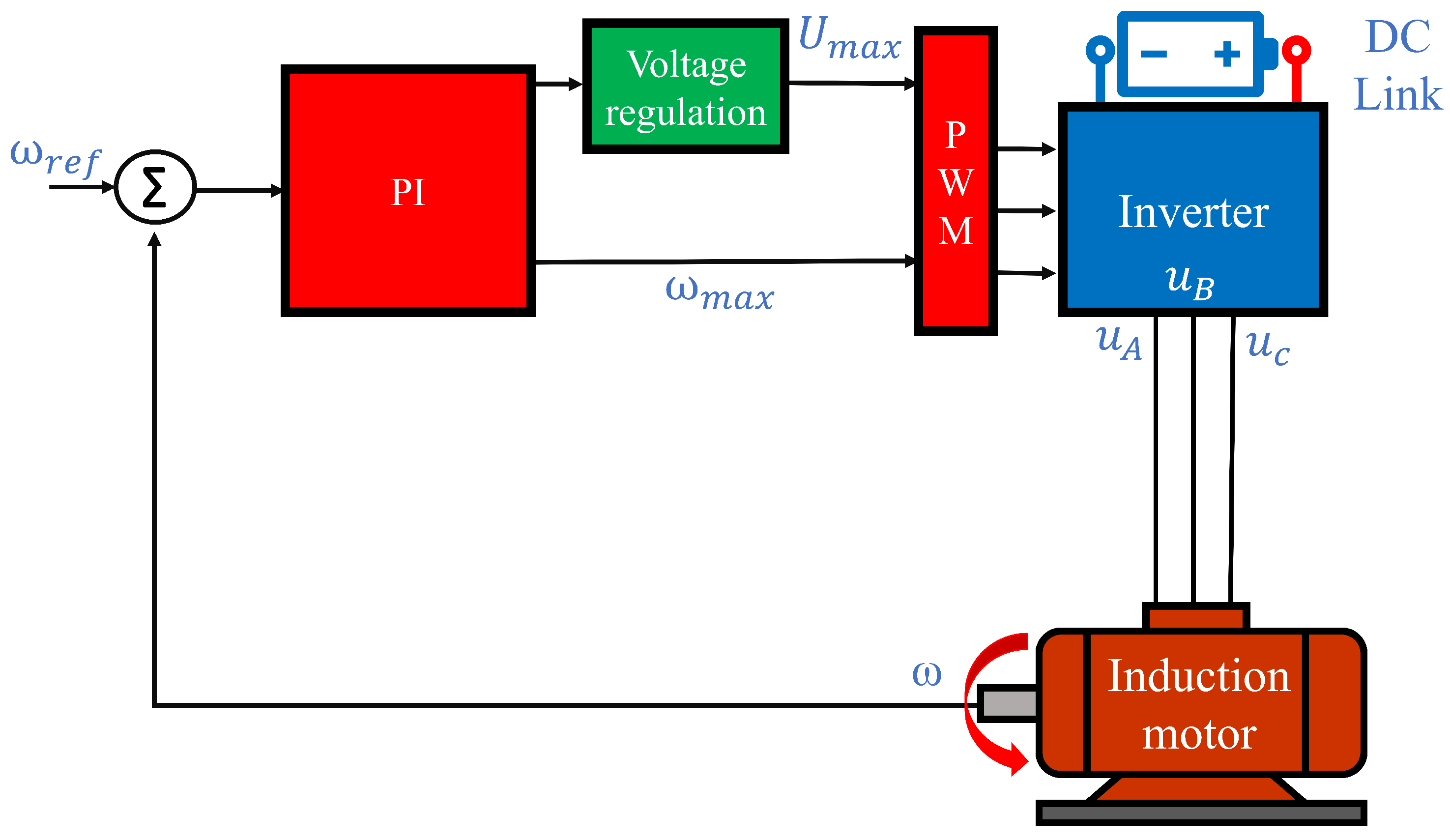
For the control of a 3-phase induction motor, a control system based on the 3-phase inverter is proposed. Such a control system consists of a 3-phase inverter supplied by a stable DC voltage from the DC link. The duty cycles of the inverter are determined according to the output signal provided by the control system. The control system can be designed as a digital control system implemented on a digital signal processor (DSP) or other digital controllers. In this particular research, the induction motor LUST ASH-22-20K13-000 is used. The used 3-phase inverter is based on the SEMIKRON Semiteach IGBT module. By using a 3-phase inverter, different motor control strategies can be applied. The same hardware configuration can be used for both scalar and vector control. To control both the torque and speed of the induction motor, different frequencies and voltages are produced through the 3-phase inverter. The used inverter consists of 6 insulated gate bipolar transistors (IGBTs), two per phase.
The schematic representation of the control system used for scalar control of the presented induction motor is presented in Figure 1. In this case, a configuration with one PI controller for angular speed is used [14].
On the other hand, the schematic representation of the control system used for vector control of the presented induction motor is presented in Figure 2.
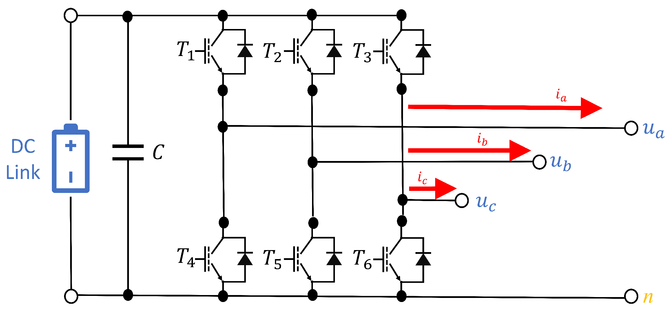
A schematic representation of the used inverter topology is presented in Figure 3.
2.2. Dataset Description
In this research, the publicly available dataset [15] was used. The used dataset is collected by measuring signals of a 3-phase inverter used in the induction motor drive system. The used drive system consists of the induction motor LUST ASH-22-20K13-000 with nominal power kW, nominal speed 3000 min, and rated phase current of A. For the control of the induction motor, a 3-phase IGBT inverter SEMIKRON Semiteach IGBT is used. The inverter is fed with a 560 V DC link with a rated output current of 30 A.
This research is carried out in two stages. The first stage is the black-box inverter model estimation, while the second is the black-box inverter compensation scheme. Both stages consist of similar identical parameters, namely: duty cycles (D), phase currents (I), direct current link voltage (), and mean phase voltages (). However, both stages have different input and output parameters. Before clarifying and defining the division into input and output parameters and which parameters belong to which stage, it is necessary to define the subscripts that are next to each variable. Each variable consists of at least two subscripts: k is the sampling step label, while , and c are labels for one of the three possible phases. The maximum previous samples reach three samples less, i.e., sample, which means that the previous three samples are taken to form the current parameter. For example, is the phase current parameter on phase c for the k sampling step. Given that signals are generally interpreted as continuous values, and this dataset is a sequence of several small recorded sequences, previous signal values are needed for training the inverter model and inverter compensation scheme. In other words, they must be included as an addition to the signal in the dataset for each generation step.
With the previously given data, it is possible to define the parameters that go into each stage of training. What was done and the input and output parameters are shown in Table 1 below.
The statistical data analysis shown in Table 2 is one of the important steps before embarking on the training process. Minimum (Min), maximum (Max), mean and standard deviation (Std) for the dataset size of 234,500 sampling steps are shown. Min indicates the minimum numerical value of the given parameter, the same applies to Max, Mean, and Std. The reason for this is an insight into the state and interrelationships of the data, which shows the complexity of the dataset itself. Furthermore, in addition to the defined symbols and their ratios between Min, Max, Mean and Std values, GP variables have been added that facilitate the subsequent definition of the results. In other words, a list of variables behind the GPSR equation (shown and defined in Section 3) is provided.
Besides the initial statistical analysis, it is important to investigate the correlation between input and output dataset variables before the implementation of AI algorithms. In this investigation, Pearson’s correlation analysis was used. As a unit of correlation measure during Pearson’s correlation analysis, Pearson’s correlation coefficient () was used. between two variables (X and Y) can be defined as:
where and represent standard deviations od variables X and Y. Furthermore, represent covariance between X and Y, defined as:
where and represent the mean values of variables X and Y. Furthermore, in this case, E represents the expectation.
The correlation value between the input and output variables can be in the to range. The value of −1.0 indicates that if the value of the input variable increases, the value of the output variable will decrease and vice versa. In case the value is equal to , then if the input variable value increases, the value of the output variable will also increase. The worst possible correlation value is 0, which means that if the value of the input variables increases or decreases, it will not influence the output variable. The results of Pearson’s correlation analysis for all dataset variables are shown in Figure A1.
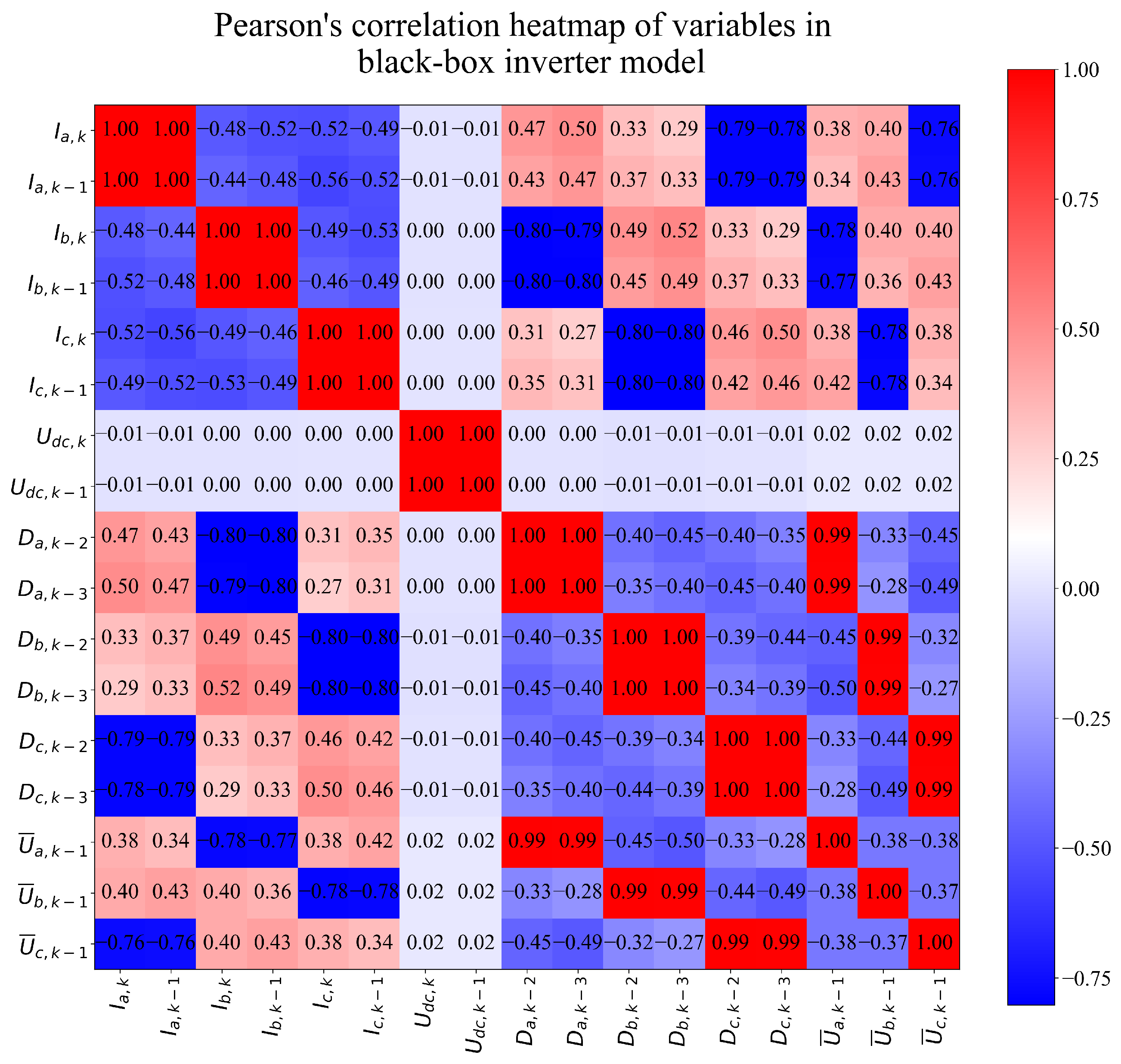
As seen from Figure A1 the variables , , , , and are mutually highly correlated. However, they do not correlate with other dataset variables. From Figure A1, it can be noticed that there is a high correlation between variables. Generally, in ML, it is favorable to have multiple highly correlated variables. However, if only one input variable is highly correlated, the GP will generate a symbolic expression containing only the highly correlated variable; others will be neglected. In the case of the black-box inverter model, the correlation between input variables and the target variables (mean phase voltages at ) should be investigated in more detail. The correlation heatmap for black-box inverter model variables is shown in Figure A2.
As seen in Figure A2, there is a high correlation between input variables and the output variables (, , ). For example, the mean phase voltage is highly correlated to , , , and . It should be noted that and have only high correlations with themselves and each other and no correlation to other variables in this model. In the case of the black-box compensation scheme, the results of Pearson’s correlation analysis are shown in the form of a heatmap in Figure A3.
In the case of the black-box compensation scheme as listed in Table 2, the target variables are duty cycles at . These target variables have an extremely high correlation (0.99) with mean phase voltages at (, , and ).
2.3. Genetic Programming–Symbolic Regression
Genetic programming–symbolic regression (GPSR) is an evolutionary algorithm that begins its execution by building a naive population that is unfit for a particular task and through the application of genetic operations for a prespecified number of generations makes them fit for a particular task [16,17]. GPSR is not a classic evolutionary algorithm since it has some similarities to classic supervised ML algorithms. For its successful execution, the GP requires the dataset with defined input and output (target) variables.
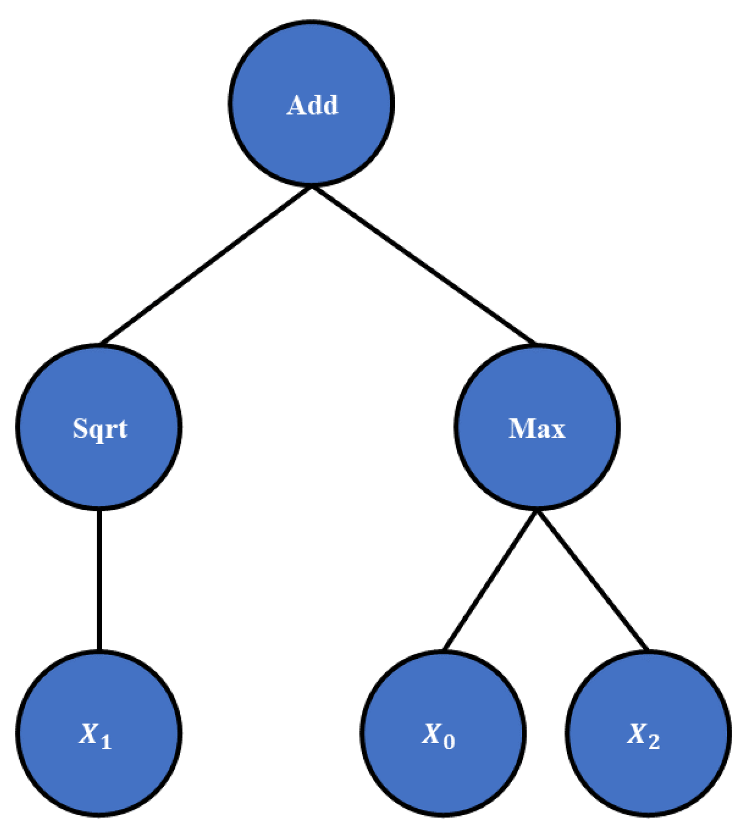
In GP, the population members are represented as tree structures. To construct the population members, the list of mathematical functions, input variables and range of constant values must be defined. The mathematical functions that will be used in this research are addition, subtraction, multiplication, division, natural logarithm, sine, cosine, tangent, minimum value, maximum value, square root, and absolute value. The constant values in GP are defined with a hyperparameter constant range and as the name states, the range of constant values is defined. As stated previously, the input and output variables are defined when the GP is applied to a specific dataset. Using the list of mathematical functions, a range of constant values, and input/output variables, the GP is developed as tree structures. The example of the initial population member in tree form is shown in Figure 4.
As seen in Figure 4, the root node is the root node “add”. At level 1, two mathematical functions are placed, i.e., “sqrt” and “max”. At level 2, only input variables are located, , , and . So the symbolic expression example has a tree depth equal to 2. Besides the symbolic expression depth in tree form, the size of the symbolic expression is measured in terms of length, i.e., the number of elements (functions, constants, and variables) that the symbolic expression contains. So the symbolic expression example has a length of 6 (3 functions and 3 input variables).
There are three commonly used methods for building an initial population in GP and these are full, grow, and ramped half-and-half methods. In this research, the method for creating the initial population ramped half-and-half method is used, which creates the initial population using full and grow methods. The term ramped refers to the depth of population tree structures to create some diversity between population members. To ensure diversity in population, the initial depth i.e., the depth of population member trees, is set in range.
Here it should be noted that the size of the population member or symbolic expression is measured in length or, in other words, the number of elements in the symbolic expression.
When the initial population is created, the population members have to be evaluated, i.e., the input variables of the training dataset are provided to calculate the output. After evaluation, the output of each population member is compared to the real one (from the dataset) to calculate the mean absolute error. In each generation, of the best population member is shown as well as the average value. After population members have been evaluated, the random selection of population members is performed. Selected members are used in tournament selection that, based on a comparison between population members, generates the winner of the tournament selection. On the winner of each tournament selection, one of four genetic operations is performed, i.e., crossover, subtree mutation, hoist, and point mutation. For crossover operation, two tournament winners are required. On the first tournament winner, the random subtree is selected, and on the second as well. Then the random subtree from the second is used and replaces the randomly selected subtree of the first tournament winner to produce the offspring of the next generation. The subtree mutation requires only one tournament winner, and the random subtree is selected, which is replaced with a randomly generated subtree using randomly chosen functions, constants, and variables. The hoist mutation randomly selects a subtree on the winner of tournament selection and on that tree randomly selects a node. Then this node is hoisted on a place of the subtree root node to create offspring of the next generation. The point mutation randomly selects nodes on the winner of the tournament selection. The constants are replaced with randomly selected constants and variables with other variables. Functions are also replaced with other functions; however, the arity of the original function must be equal to the new function.
The stopping criteria and the maximum number of generations are two termination criteria that can be used to stop the execution of GP. The stopping criteria are the lowest predefined value of the fitness function, and if the value is reached by one of the population members during GP execution, it would terminate the GP execution. However, in this paper, the idea was to stop the execution when a maximum number of generations is reached to lower the fitness function value as much as possible. So the stopping criteria were set to a very low value. The parsimony coefficient is one of the most important GP hyperparameters, and it is responsible for the prevention of the bloat phenomenon. In cases where the correlation between dataset variables is low or nonexistent, the GP will try to build the relationship between variables by increasing the size of the population members to lower the fitness function value. However, if the value of the fitness function is not lowered and the size of the population members grows rapidly from generation to generation, then the bloat phenomenon occurs. This phenomenon can have a negative effect on the GP execution time, i.e., it can prolong the execution and it can cause resource exhaust error. This coefficient tries to lower the increases of the fitness function valueof large population members during the GP tournament selection and in this way, makes large population members less favorable for winning the tournament selection process. This is the most sensitive parameter, i.e., a large value can choke the population, which can lead to poor estimation accuracy of obtained symbolic expression, while a small value can cause the bloat phenomenon.
2.4. Research Methodology
To construct the highest-performing symbolic expression for the estimation of phase voltages and duty cycles, per each phase a GP procedure with a random hyperparameter search was performed. The random search is executed for multiple iterations until termination criteria are met. A graphical representation of the GPSR process with a random parameter search for one case is presented in Figure 5.
The ranges of each GPSR hyperparameter used in this research throughout all GPSR execution are listed in Table 3.
It should be noted that the range of each hyperparameter listed in Table 3 is defined through the initial tuning of each GPSR hyperparameter. The population size hyperparameter was set to the 100–500 range since a larger population causes longer execution times, while too low (below 100) can cause bad performance, i.e., faster executions with low estimation accuracy of obtained symbolic expression. The number of generations was set to the 100–200 range since in this range, GPSR produces the symbolic expression for the estimation of mean phase voltages and duty cycles with pretty high accuracy. It should be noted that this hyperparameter was the main termination criterion for GPSR execution since the predefined value of the stopping criteria (lowest value of the fitness function) was never reached by any of the population members.
The tournament size was arbitrarily set to the 10–50 range. The depth of population members in tree form was set to the 3–15 range. Since this hyperparameter is defined with two values (lower and upper), the idea was to ensure the larger diversity in the initial population as possible without drastically prolonging execution times.
The crossover and the other three mutation operations were set to a very generic range (–1) to see which one of these genetic operators will be dominating the evolution process. It is generally suggested in GP that the sum of all genetic operators is equal to 1; otherwise, some tournament selection winners might enter the next generation unchanged. However, in the initial investigation, it was shown that presetting one of the genetic operations equal to (or higher) and the sum of all genetic operations equal to 1 can result in longer GPSR execution times. So, the range between and 1 in the hyperparameter search method proved to be the best for this investigation.
The maximum number of samples range, i.e., the training dataset size used to evaluate each population member, was set to to 1. Lowering the value of the max samples probably would not have any effect since the dataset has a large number of samples.
The constant range hyperparameter range was set to – to ensure that the random hyperparameter search method would randomly select the large constant range, which in GPSR would be used for the initial population and later for mutation operations.
One of the most sensitive hyperparameters in the entire investigation conducted in this paper is the parsimony coefficient. The range which was later used in the random hyperparameter search method had to be carefully studied since very small values (for example ) could cause memory overflow, while large values (for example 1, 2, 10, etc.) could cause poor estimation performance for the obtained symbolic expressions. In other words, small parsimony coefficients do not penalize large population members, and they continue to grow from generation to generation without any benefit to the fitness function value. The high value of the parsimony coefficient is choking the evolution process by hardly penalizing the fitness function of larger programs, in this way making them less favorable for the tournament selection process. This coefficient had to be differently configured for mean phase voltages investigation and differently for duty cycles investigation. In the case of mean phase voltages investigation, the range of parsimony coefficient was set to the – range. In the case of duty cycles investigation, the range was set to the – range since larger values were preventing the growth of the population members.
To evaluate the estimation performance results of the constructed symbolic expressions, three different metrics were used. All three metrics are based on the comparison of real and estimated output data. The first evaluation metric used is the score or the coefficient of determination [18]. Two other used metrics are [19] and [20].
To evaluate generalization performances of the constructed symbolic expressions, 5-fold cross-validation is used. The entire dataset is divided into five equally large folds. Five different cases are examined. In each case, four folds are used to form a training dataset, while the remaining one is used for model testing. In each case, a different fold is used for model testing. The process is repeated five times until all combinations have been observed. A graphical representation of a 5-fold cross-validation is presented in Figure 6.
To evaluate both estimation and generalization procedures, mean values of used metrics and their standard deviations are used. Mean values and standard deviations are determined by using results achieved during the cross-validation procedure. For the case of , the aim is to achieve closer to 1. For the case of and the aim is to achieve the lowest possible value. On the other hand, the symbolic expressions with the lowest standard deviation can be considered the best-performing models from a generalization standpoint. Such a conclusion can be derived regardless of the metric used.
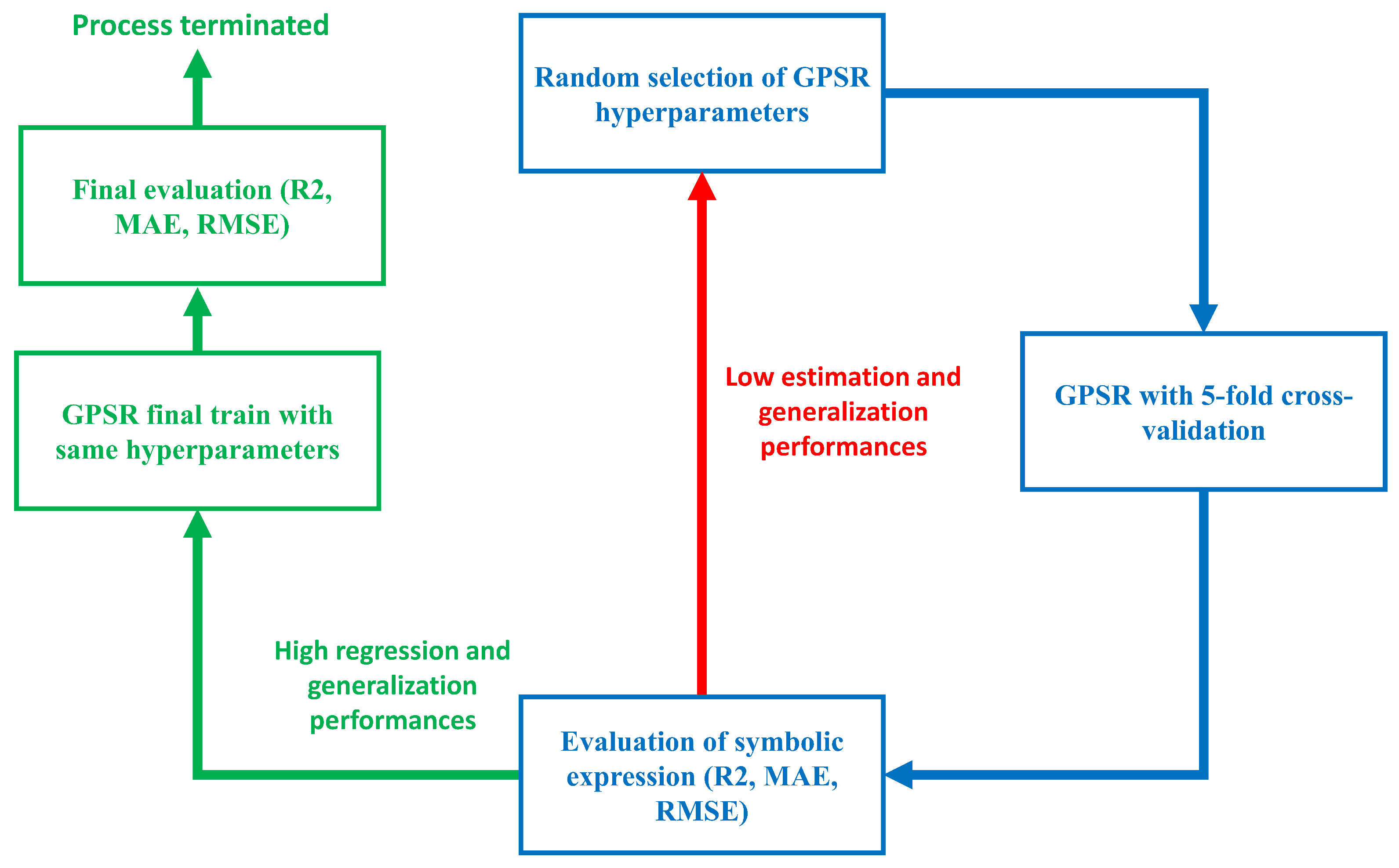
Finally, the entire procedure of GPSR with the random hyperparameter search method and 5-fold cross validation is shown in the following Figure 7.
The process shown in Figure 7 can be described in the following steps:
- The process begins with a random selection of GPSR hyperparameters;
- Then these hyperparameters are used in GPSR with 5-fold cross-validation execution, where 5 different symbolic expressions are obtained (one for each execution);
- Then each symbolic expression is evaluated on training and validation dataset to determine the mean and standard deviation values of , , and metrics.
- If the mean value of is higher than , the process continues to the final training with the same hyperparameters used in 5-fold cross validation. If not, the process starts from the beginning by selecting random hyperparameters.
- In the case of GPSR final training with the same hyperparameters, the GPSR is trained on the training part of the dataset ( of the original dataset).
- After the symbolic expression is obtained, it is evaluated on training and testing parts of the original dataset to calculate the mean and standard deviation values of , , and . If the value of is larger than , the values of and are lower than 5 and if the standard deviations of the aforementioned metrics are lower than , then the process is successfully terminated.
It should be noted that in the following section, the best symbolic expression obtained for each output variable was obtained at the final GPSR stage after 5-fold cross validation was successfully passed.
2.5. Computational Resources
All investigations were conducted on the computer with an Intel I7-4470 CPU and 16 GB of DDR3 RAM. All codes were written in Python programming language (version 3.9.13). The GPSR was used from the gplearn library (version 0.4.2), and the evaluation metric was used from the scikit-learn library (version 1.2.0). The random hyperparameter search and 5-fold cross-validation method were written from scratch using a built-in random library.
3. Results and Discussion
In this section, the results achieved for both phase voltages and duty cycle estimation are presented and discussed.
3.1. Estimation of Phase Voltages
For each phase, the GPSR hyperparameters used to achieve the symbolic expression with the highest estimation performances are shown in Table 4. From the presented hyperparameters, it can be seen that for the case of all three phases, the best hyperparameters are positioned roughly on the middle value in the possible value interval.
From Table 4, it can be noticed that in the Phase A case, the hoist mutation was dominating the genetic operation, while for phase B and phase C, the subtree mutation was the dominating genetic operation. The stopping criteria were prespecified to a very low value (low ), and since they were never met by any of the population members, the GPSR stopped the execution after the predefined maximum number of generations was reached. Due to the small parsimony coefficient values, all three symbolic expressions for the estimation of mean phase voltages are large, and their lengths are equal to 107, 180, and 300, respectively. This means that the equations consist of 107, 180, and 300 elements, respectively. If the presented hyperparameters are used for GP execution, for phase A, the symbolic expression
is constructed. The presented equation is derived from the generated symbolic expression obtained during the execution of GP. Equation (3) consists of , , , , , , , , and input variables. Looking at Table 2, these input variables are duty cycles at k − 3, , , , , , and , and are required to calculate the mean phase voltage . From Figure A2, it can be seen that all required variables do not have a high correlation with the target variable. The lowest correlation values with the target variable have variables , and . In this case, the correlation is equal to 0.02 for both variables.
Furthermore, if the hyperparameters from the second column are used, the symbolic expression
is determined for phase B. Equation (4) requires all input variables except for the or DC-link voltage at k () variable. The variable correlates with the target variable equal to 0.02. The expression is derived by using variation methods during GP execution. Finally, if the hyperparameters from the last are used during GP execution, the symbolic expression for the third phase
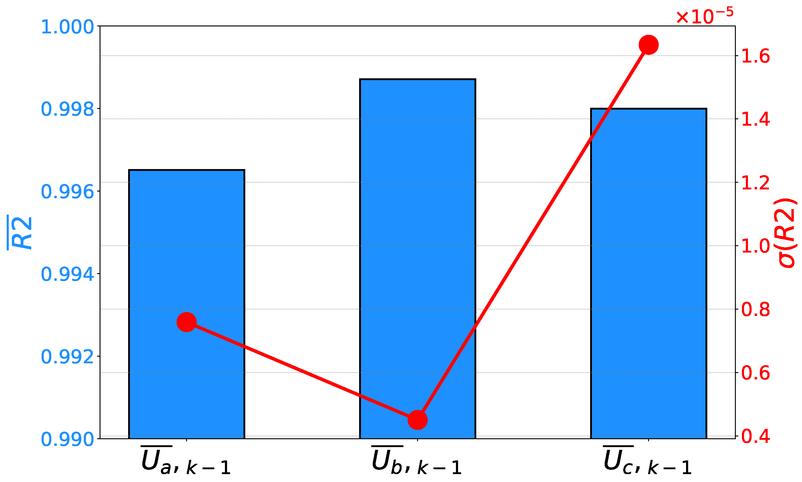
is defined. Equation (5) requires all input variables to calculate the output, and it is obtained at the end of GP execution. If the achieved mean values and their standard deviations are compared for each phase, it can be noticed that the highest is achieved for the second phase. Furthermore, the second phase is characterized by the lowest , pointing toward the conclusion that has the highest generalization performance results. For phases A and C, high regression and generalization performance results are also achieved, as presented in Figure 8.
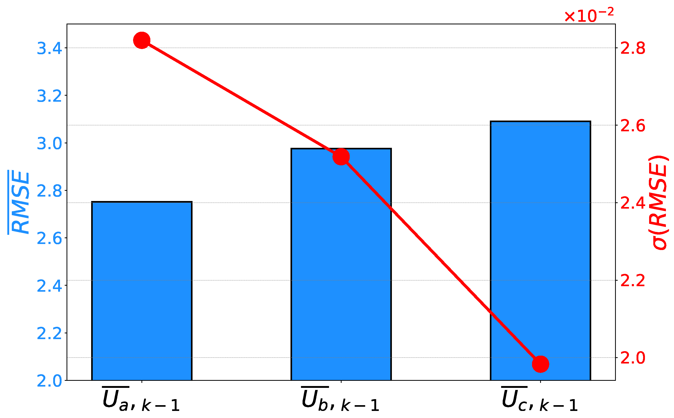
If the error rates are compared, a similar conclusion can be derived. In this case, phase B is characterized by the lowest error rates. At the same time, phase B has the lowest and values. Such a result is pointing toward the conclusion that the symbolic expression for has the highest generalization performance results. Similar to the case of , the expressions for the other two phases still have high estimation and generalization performance results, as can be seen in Figure 9 and Figure 10.
3.2. Estimation of Duty Cycles
When GP is used for the construction of symbolic expressions for the estimation of duty cycles per each phase, the highest estimation and generalization performance results are achieved if the GP hyperparameters presented in Table 5 are used. As it is in the case of voltage estimation, the highest performing symbolic expressions are achieved if the hyperparameters from the middle of the hyperparameter interval are used.
From Table 5 it can be seen that the population size hyperparameter value was the largest in the Phase A case. The dominating genetic operation for Phase A was subtree mutation, for Phase B, it was hoist mutation, and for Phase C, it was subtree mutation. The parsimony coefficient, as planned, has an extremely low value when compared to the parsimony coefficient values used in the mean phase voltages case. The main reason for choosing extremely low values in the duty cycles case is that some variables have extremely high (–1) correlations to the targeted variables. This can have a negative effect during GPSR execution since it can prevent the evolution process of the population members due to a strong correlation between specific variables.
The parsimony coefficient in this case had a low influence and generated relatively large symbolic expressions. The size of first two symbolic expressions , and (in terms of length) are 29 and 250. The smallest symbolic expression was obtained in the case of , where the initial form contains 17 elements, and after simplifying the expression, the symbolic expression consists of 10 elements.
If the given hyper-parameters are used for GPSR execution, for phase A, the symbolic expression
is constructed. Equation (6) consists of all input variables except for , and from Table 2, it can be seen that this variable is mean phase voltage . Looking at Figure A3, this variable does not have an extremely high correlation to the target variable. The correlation is equal to −0.45. Furthermore, if the hyper-parameters from the second column are used, the symbolic expression
is determined for phase B. Equation (7) consists of all input variables except for , and . From Table 2, it can be noticed that these variables are , , and . From Figure A3, these three variables have correlation values with target variables equal to , , and , respectively. So, these variables have a high correlation with the target variable, although it is interesting that they were not included in the symbolic expression. Finally, if the hyper-parameters from the last are used during GPSR execution, the symbolic expression for the third phase:
is defined. Equation (8) consists of four input variables, , , , and . From Table 2, it can be seen that these variables are , , , and , respectively. From Figure A3, it can be seen that these variables have a high correlation with the target variable except for , which has a value of .
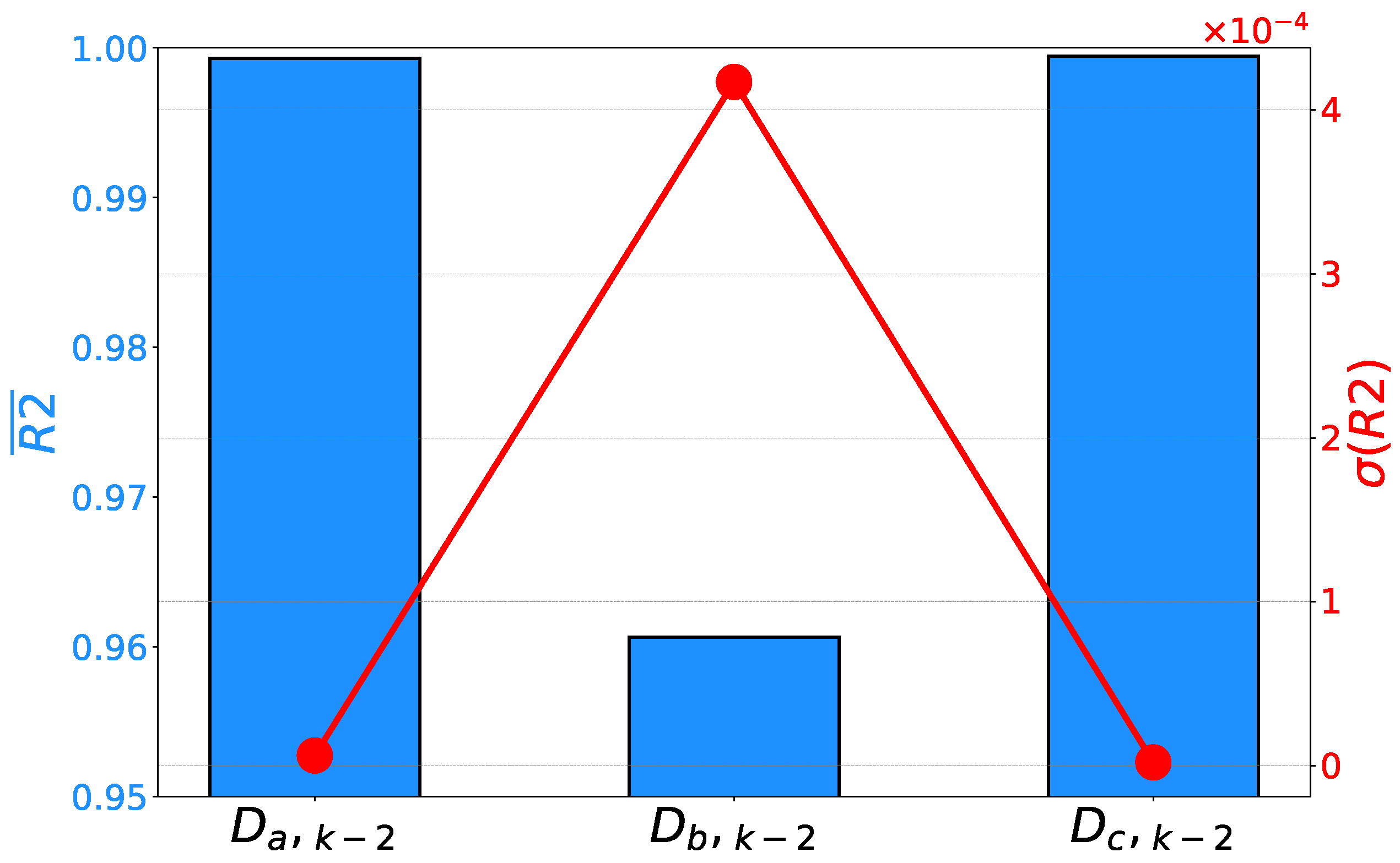
If the performance results of the presented symbolic expressions are observed, it can be noticed that the lowest values are achieved on the estimation of the duty cycle for phase B. At the same time, the same symbolic expression has the lowest generalization performance. Such a conclusion can be derived from the highest standard deviation. It is interesting to notice that the maximal score achieved with is significantly lower than in the case of other symbolic expressions, even those for voltage estimation. If the estimation and generalization performance results of and are observed, significantly higher results are achieved, as presented in Figure 11.
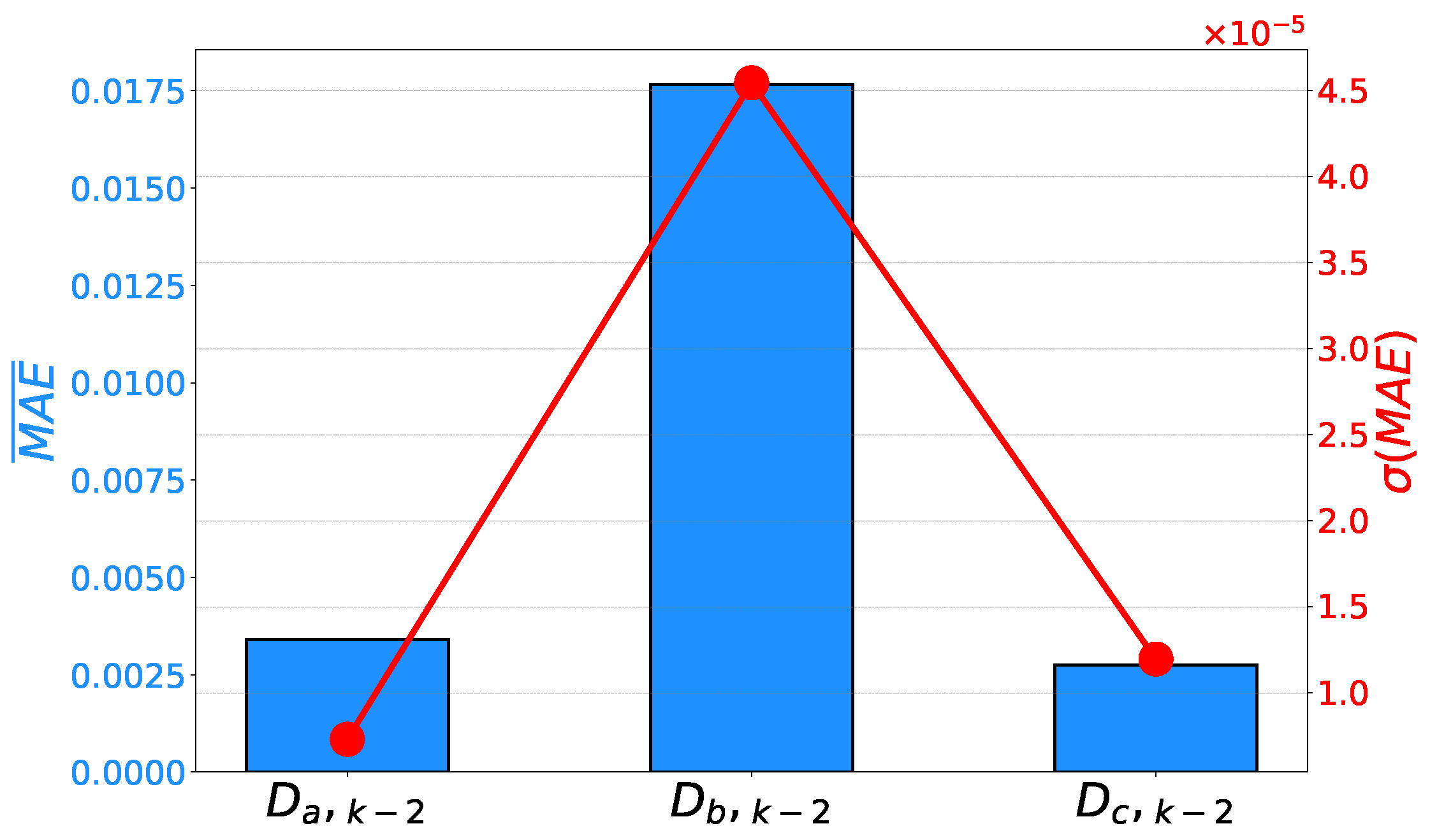
A similar relationship can be noticed if the achieved mean error rates and their standard deviations are compared. It can be noticed that has achieved significantly higher error rates. Furthermore, the same symbolic expression has achieved higher and , pointing toward lower generalization performance results. Symbolic expressions for phases A and C are characterized by lower error rates, as presented in Figure 12 and Figure 13.
From the presented results, it can be seen that by using GPSR, symbolic expressions characterized by high estimation and generalization performance results can be designed.
3.3. Comparison between Symbolic Regression and Other Modeling Methods
To conclude whether the method applies to a problem, it is necessary to compare the proposed method with other similar methods. This was performed using a tabular representation, presented in Table 6. Three approaches were chosen: the proposed GPSR method, ML methods, and deterministic methods. ML methods in the last few years and even decades have been solutions for complex problems, whether it is a classification, regression, or any other kind of problem, depending on the desired solution. Deterministic methods provide an exact solution based on defined rules, and it is important to take this into account as a potential solution. Additionally, five criteria were selected that must be met to select the appropriate algorithm:
- Model complexity: Refers to the structure of the model itself, and how many parameters it contains, for example, models such as multilayer perceptron (MLP) or convolutional neural network (CNN) are black-box models, that is, the user is not aware of what is happening at a certain moment during training and cannot influence it before the results are calculated. Only the input and output are known.
- Model performance: Indicates what the user wants, which is what kind of performance a particular algorithm showed, that is, how high-quality the obtained results are.
- Model execution time: Refers to the time of execution or obtaining results from the moment of starting the model estimation process.
- Modeling procedure complexity: The complexity when creating an algorithm to perform a certain task.
- Modeling computational complexity: The hardware requirement, i.e., how many resources each model uses to perform the task.
In addition to GPSR, ML methods and conventional deterministic methods were taken into account. ML methods are quite complex methods and are mainly used as black-box models. Deterministic modeling methods are of medium difficulty. Various mathematical equations describe relationships and potential future values that can be predicted for a given issue, but there are cases that deterministic methods are rejected because the deviation from the real value has too much oscillation. Contrary to the two competitors, the complexity of GPSR is extremely low, the entire structure of the algorithm is visible, and it is much easier to influence the algorithm itself than other compared methods. As far as model performance is concerned, all three approaches can achieve top results, and one against the others does not pose a challenge. Model execution time is one of the key factors for choosing a method to solve a certain problem. In this case, GPSR gives the fastest result from the beginning of the estimation initialization to its completion, compared to ML and deterministic methods. The reason for this is that with GPSR, the final result is a single equation that describes the system almost perfectly, which was confirmed by the results of this research. Regarding the complexity of the procedure, GPSR and ML models have a low complexity rate for algorithm preparation. The reason for this is that for most ML algorithms, there are already publicly available programming libraries that are easy to implement. In the end, it remains to compare the computational complexity of all three approaches. It can be seen that deterministic models have the least computational complexity, while GPSR and ML models, it is high. The reason for this is the complexity of the dataset and the desired performance of the model. For the output results to be reliable and accurate, more demanding hyperparameters must be defined, which results in higher hardware requirements for the execution of the task.
4. Conclusions
In this paper, an approach for drive inverter modeling based on GPSR utilization is presented. Such an approach can offer a stable estimation performance by maintaining simple and low-memory models based on symbolic expressions. According to the results and the research hypothesis, the following can be stated:
- It is possible to utilize GP to design symbolic expressions for drive inverter modeling.
- The expressions have high performance for both black-box model and black-box compensation scheme targets.
- By using hyper-parameters selected with a random selection process, high estimation and generalization performance results are achieved.
The advantages of this approach are as follows:
- The obtained symbolic expressions are simple and easier to use than complex, trained AI/ML models.
- The symbolic expressions do not require all input variables to calculate the desired output. So further investigation using this approach could result in symbolic expression with fewer input variables.
- The process of training the GPSR even with 5-fold cross validation is on average 60 min. It can be stated that the presented execution time is not too long to obtain quality and robust symbolic expressions with high estimation accuracy.
The disadvantages of this approach are as follows:
- Initial tuning and defining hyperparameter ranges of the GPSR algorithm is a painstaking process that has to be carefully planned and executed. If this stage is done properly, then the GPSR with random hyperparameter search and the 5-fold cross-validation method should run smoothly. However, the process of fine-tuning to define hyperparameter ranges is a time-consuming process since each hyperparameter has to be defined and the GPSR must be executed to see the hyperparameter’s influence on the performance of the GPSR algorithm.
- The extremely high correlation between some dataset variables has presented a problem during the investigation since these highly correlated variables prevented the evolution process of GPSR.
- The tuning of the parsimony coefficient is the most sensitive process since the small variation of this value could cause a negative effect on GPSR algorithm execution (higher execution times, and lower accuracy of obtained symbolic expressions).
Future work will be based on the implementation of developed symbolic expressions into more complex ensemble models. Alongside the implementation of more complex regression methods, the authors will examine the performance of the proposed method on other inverter models. Furthermore, the physical drive system and inverter will be designed and implemented to experimentally verify the performance of the proposed method. The developed drive system and inverter will be used to collect a new dataset that will be used to create the new estimation models. Alongside new data collection, the possibility of the inclusion of new input variables will be examined.
Author Contributions
Conceptualization, M.G., N.A. and I.L.; methodology, M.G. and S.B.Š.; software, N.A. and M.G.; validation, M.G., I.L. and S.B.Š.; formal analysis, M.G. and S.B.Š.; investigation, M.G., N.A. and S.B.Š.; resources, N.A. and I.L.; data curation, M.G. and S.B.Š.; writing—original draft preparation, M.G., N.A. and I.L.; writing—review and editing, M.G., N.A. and S.B.Š.; visualization, I.L. and S.B.Š.; supervision, N.A. and I.L.; project administration, N.A. and S.B.Š.; funding acquisition, N.A. and I.L. All authors have read and agreed to the published version of the manuscript.
Funding
This research has been (partly) supported by the CEEPUS network CIII-HR-0108, European Regional Development Fund under the grant KK.01.1.1.01.0009 (DATACROSS), project CEKOM under the grant KK.01.2.2.03.0004, Erasmus+ project WICT under the grant 2021-1-HR01-KA220-HED-000031177, and University of Rijeka scientific grant uniri-tehnic-18-275-1447.
Institutional Review Board Statement
Not applicable.
Informed Consent Statement
Not applicable.
Data Availability Statement
Github repository with the complete program code used to realize this research: https://github.com/nandelic2022/InverterGP (accessed date: 30 December 2022).
Conflicts of Interest
The authors declare no conflict of interest.
Appendix A
Figure A1.
The results of Pearson’s correlation analysis for all dataset variables.

Figure A2.
The Pearson’s correlation heatmap for variables in black-box inverter model.

Figure A3.
The Pearson’s correlation heatmap of dataset variables used in black-box compensation scheme model.
Figure A3.
The Pearson’s correlation heatmap of dataset variables used in black-box compensation scheme model.

References
- Robles, E.; Fernandez, M.; Andreu, J.; Ibarra, E.; Ugalde, U. Advanced power inverter topologies and modulation techniques for common-mode voltage elimination in electric motor drive systems. Renew. Sustain. Energy Rev. 2021, 140, 110746. [Google Scholar] [CrossRef]
- Chung, H.S.; He, Y.; Huang, M.; Wu, W.; Blaabjerg, F. Control and Filter Design of Single-Phase Grid-Connected Converters; John Wiley & Sons: Hoboken, NJ, USA, 2022. [Google Scholar]
- Gaddala, R.K.; Majumder, M.G.; Rajashekara, K. DC-Link Voltage Stability Analysis of Grid-Tied Converters Using DC Impedance Models. Energies 2022, 15, 6247. [Google Scholar] [CrossRef]
- Rafiq, M.A.; Ulasyar, A.; Uddin, W.; Zad, H.S.; Khattak, A.; Zeb, K. Design and Control of a Quasi-Z Source Multilevel Inverter Using a New Reaching Law-Based Sliding Mode Control. Energies 2022, 15, 8002. [Google Scholar] [CrossRef]
- Vishnuram, P.; Ramachandiran, G.; Sudhakar Babu, T.; Nastasi, B. Induction Heating in Domestic Cooking and Industrial Melting Applications: A Systematic Review on Modelling, Converter Topologies and Control Schemes. Energies 2021, 14, 6634. [Google Scholar] [CrossRef]
- Ashraf, N.; Abbas, G.; Ullah, N.; Alahmadi, A.A.; Awan, A.B.; Zubair, M.; Farooq, U. A Simple Two-Stage AC-AC Circuit Topology Employed as High-Frequency Controller for Domestic Induction Heating System. Appl. Sci. 2021, 11, 8325. [Google Scholar] [CrossRef]
- Ramkumar, S.; Kamaraj, V.; Thamizharasan, S. GA based optimization and critical evaluation SHE methods for three-level inverter. In Proceedings of the 2011 1st International Conference on Electrical Energy Systems, Chennai, India, 3–5 January 2011; pp. 115–121. [Google Scholar]
- Cheng, F.F.; Yeh, S.N. Application of fuzzy logic in the speed control of AC servo system and an intelligent inverter. IEEE Trans. Energy Convers. 1993, 8, 312–318. [Google Scholar] [CrossRef]
- Aziz, M.V.G.; Questera, N.; Hindersah, H. Speed Profile Algorithm using Artificial Intelligence for Vehicle Control Unit on Quest Motors Electric Vehicles. In Proceedings of the 2022 7th International Conference on Electric Vehicular Technology (ICEVT), Online, 14–16 September 2022; pp. 200–204. [Google Scholar]
- Khan, A.A.; Beg, O.A.; Alamaniotis, M.; Ahmed, S. Intelligent anomaly identification in cyber-physical inverter-based systems. Electr. Power Syst. Res. 2021, 193, 107024. [Google Scholar] [CrossRef]
- Anđelić, N.; Lorencin, I.; Glučina, M.; Car, Z. Mean Phase Voltages and Duty Cycles Estimation of a Three-Phase Inverter in a Drive System Using Machine Learning Algorithms. Electronics 2022, 11, 2623. [Google Scholar] [CrossRef]
- Rajeswaran, N.; Swarupa, M.L.; Rao, T.S.; Chetaswi, K. Hybrid artificial intelligence based fault diagnosis of svpwm voltage source inverters for induction motor. Mater. Today Proc. 2018, 5, 565–571. [Google Scholar] [CrossRef]
- Anđelić, N.; Šegota, S.B.; Lorencin, I.; Jurilj, Z.; Šušteršič, T.; Blagojević, A.; Protić, A.; Ćabov, T.; Filipović, N.; Car, Z. Estimation of covid-19 epidemiology curve of the united states using genetic programming algorithm. Int. J. Environ. Res. Public Health 2021, 18, 959. [Google Scholar] [CrossRef] [PubMed]
- Stender, M.; Wallscheid, O.; Böcker, J. Data Set Description: Three-Phase IGBT Two-Level Inverter for Electrical Drives, the Dataset Used in the Research and Publicly Available on the Kaggle Repository; Department of Power Electronics and Electrical Drives, Paderborn University: Paderborn, Germany, 2020. [Google Scholar]
- Stender, M.; Wallscheid, O.; Boecker, J. Comparison of gray-box and black-box two-level three-phase inverter models for electrical drives. IEEE Trans. Ind. Electron. 2020, 68, 8646–8656. [Google Scholar] [CrossRef]
- Huang, Z.; Mei, Y.; Zhong, J. Semantic linear genetic programming for symbolic regression. IEEE Trans. Cybern. 2022, 1–14. [Google Scholar] [CrossRef] [PubMed]
- Nicolau, M.; McDermott, J. Genetic programming symbolic regression: What is the prior on the prediction? In Genetic Programming Theory and Practice XVII; Springer: Cham, Switzerland, 2020; pp. 201–225. [Google Scholar]
- Plonsky, L.; Ghanbar, H. Multiple regression in L2 research: A methodological synthesis and guide to interpreting R2 values. Mod. Lang. J. 2018, 102, 713–731. [Google Scholar] [CrossRef]
- Qi, J.; Du, J.; Siniscalchi, S.M.; Ma, X.; Lee, C.H. On mean absolute error for deep neural network based vector-to-vector regression. IEEE Signal Process. Lett. 2020, 27, 1485–1489. [Google Scholar] [CrossRef]
- Chai, T.; Draxler, R.R. Root mean square error (RMSE) or mean absolute error (MAE)?–Arguments against avoiding RMSE in the literature. Geosci. Model Dev. 2014, 7, 1247–1250. [Google Scholar] [CrossRef] [Green Version]
Figure 1.
Schematics of the control system.

Figure 2.
Schematics of the control system.

Figure 3.
Schematics for used 3-phase inverter.

Figure 4.
The example of symbolic expression in tree form.

Figure 5.
The dataflow of GP with random parameter search for the case of estimation.

Figure 6.
Graphical representation of 5-fold cross-validation procedure.

Figure 7.
The flowchart of GPSR with random hyperparameter search and 5-fold cross validation.

Figure 8.
Mean scores and their standard deviations achieved on the prediction of phase voltages.

Figure 9.
Mean scores and their standard deviations achieved on the prediction of phase voltages.

Figure 10.
Mean scores and their standard deviations achieved on the prediction of phase voltages.

Figure 11.
Mean scores and their standard deviations achieved on the prediction of duty cycles.

Figure 12.
Mean scores and their standard deviations achieved on the prediction of duty cycles.

Figure 13.
Mean scores and their standard deviations achieved on the prediction of duty cycles.


Table 1.
Input and output parameters for both research models (: duty cycle phase A; : duty cycle phase B; : duty cycle phase C; : current phase A; : current phase B; : current phase C; : voltage phase A; : voltage phase B; : voltage phase C; : DC-link voltage).
Table 1.
Input and output parameters for both research models (: duty cycle phase A; : duty cycle phase B; : duty cycle phase C; : current phase A; : current phase B; : current phase C; : voltage phase A; : voltage phase B; : voltage phase C; : DC-link voltage).
| Black-Box Inverter Model | Black-Box Inverter Compensation Scheme | ||
|---|---|---|---|
| Inputs | Outputs | Inputs | Outputs |
Table 2.
The list of input and output variables that were used in GP for the black-box inverter model and black-box compensation scheme. The symbolic representation of input and output variables in GP was given as well as the results of statistical analysis (minimum, maximum, mean and standard deviation values) for each variable.
| Symbol | GP Variable | Min | Max | Mean | Std | ||
|---|---|---|---|---|---|---|---|
| Black-Box Inverter Model | Duty cycles at | 0 | 1 | 0.5 | 0.21 | ||
| 0 | 1 | 0.50026 | 0.21 | ||||
| 0 | 1 | 0.5 | 0.21 | ||||
| Duty cycles at | 0 | 1 | 0.5 | 0.21 | |||
| 0 | 1 | 0.5 | 0.21 | ||||
| 0 | 1 | 0.5 | 0.21 | ||||
| Phase currents | −7.3 | 7.47 | 0.0005 | 2.19 | |||
| −6.32 | 6.66 | −0.007 | 2.15 | ||||
| −7.113 | 7.437 | −0.008 | 2.21 | ||||
| Phase currents at k | −7.47 | 7.47 | 0.0005 | 2.19 | |||
| −6.32 | 6.668 | −0.007 | 2.15 | ||||
| −7.1123 | 7.437 | −0.008 | 2.21 | ||||
| DC-link voltage at k − 1 | 548.013 | 575.55 | 567.13 | 4.99 | |||
| DC-link voltage at k | 548.013 | 575.55 | 567.13 | 4.99 | |||
| Mean Phase Voltages at | −2.28 | 573.33 | 283.41 | 114.64 | |||
| −2.087 | 573.2 | 283.46 | 114.29 | ||||
| −2.31 | 573.17 | 283.74 | 114.6 | ||||
| Black-box inverter compensation scheme | Mean Phase voltage at | −2.288 | 573.33 | 283.41 | 114.6 | ||
| −2.088 | 573.2 | 283.46 | 114.2 | ||||
| −2.31 | 573.17 | 283.74 | 114.6 | ||||
| Phase current | −7.3 | 7.47 | 0.0005 | 2.19 | |||
| −6.32 | 6.668 | −0.007 | 2.15 | ||||
| −7.11 | 7.437 | −0.008 | 2.21 | ||||
| Phase current | −7.3 | 7.47 | 0.0005 | 2.19 | |||
| −6.32 | 6.668 | −0.007 | 2.15 | ||||
| −7.113 | 7.437 | −0.008 | 2.21 | ||||
| DC-link voltage | 548.013 | 575.55 | 567.13 | 4.99 | |||
| DC-link voltage | 548.013 | 575.55 | 567.13 | 4.99 | |||
| Duty cycles | 0 | 1 | 0.5 | 0.21 | |||
| 0 | 1 | 0.5 | 0.21 | ||||
| 0 | 1 | 0.5 | 0.21 |
Table 3.
The range of GPSR hyperparameters used in this research.
| Hyperparameter Name | Upper Bound | Lower Bound |
|---|---|---|
| Population size | 100 | 500 |
| Number of generations | 100 | 200 |
| Tournament size | 10 | 50 |
| Init depth | (3–7) | (8–15) |
| Crossover coefficient | 0.001 | 1 |
| Subtree mutation | 0.001 | 1 |
| Hoist Mutation | 0.001 | 1 |
| Point Mutation | 0.001 | 1 |
| Stopping criteria | 0 | |
| Maximum samples | 0.99 | 1 |
| Constant range | −10,000 | 10,000 |
| Parsimony coefficient (mean phase voltages) | ||
| Parsimony coefficient (duty cycles) |
Table 4.
The GPSR hyperparameters used for the definition of the symbolic expressions for phase voltage estimation.
Table 4.
The GPSR hyperparameters used for the definition of the symbolic expressions for phase voltage estimation.
| Phase A | Phase B | Phase C | |
|---|---|---|---|
| Population size | 343 | 313 | 254 |
| Number of generations | 143 | 166 | 188 |
| Tournament selection size | 19 | 10 | 23 |
| Initial depth | (3, 9) | (3, 8) | (3, 10) |
| Crossover coefficient | 0.12793209 | 0.046102316 | 0.069413606 |
| Subtree mutation coefficient | 0.282640797 | 0.637264456 | 0.746384432 |
| Hoist mutation coefficient | 0.396828111 | 0.105422777 | 0.02853356 |
| Point mutation coefficient | 0.029499366 | 0.205518506 | 0.155416003 |
| Stopping criteria | 0.000318147 | 0.000915282 | 0.000625943 |
| Maximal number of samples | 0.958912563 | 0.902661416 | 0.906783421 |
| Constant range | (−5221.42, 6286.92) | (−5539.63, 2462.81) | (−5206.02, 6947.92) |
| Parsimony coefficient | 0.000715945 | 0.000944609 | 0.000823575 |
Table 5.
The genetic programming parameters used for the definition of the symbolic expressions for duty cycles estimation.
Table 5.
The genetic programming parameters used for the definition of the symbolic expressions for duty cycles estimation.
| Phase A | Phase B | Phase C | |
|---|---|---|---|
| Population size | 498 | 258 | 299 |
| Number of generations | 167 | 171 | 121 |
| Tournament selection size | 28 | 47 | 44 |
| Initial depth | (6, 15) | (7, 9) | (3, 9) |
| Crossover coefficient | 0.216988623 | 0.07 | 0.05 |
| Subtree mutation coefficient | 0.29 | 0.22879136 | 0.72 |
| Hoist mutation coefficient | 0.143122346 | 0.334293786 | 0.048 |
| Point mutation coefficient | 0.270236321 | 0.047146706 | 0.085 |
| Stopping criteria | |||
| Maximal number of samples | 0.990992282 | 0.994145103 | 0.999404119 |
| Constant range | (−9955.02, 2292.48) | (−8145.73, 1432.6) | (−7631.24, 5066.85) |
| Parsimony coefficient |
Table 6.
The cost comparison of GPRS modeling, ML modeling, and deterministic modeling.
| GPSR Modeling | ML Modeling | Deterministic Modeling | |
|---|---|---|---|
| Model complexity | Low | High | Medium |
| Model performances | High | High | High |
| Model execution time | Low | High | Medium |
| Modeling procedure complexity | Low | Low | Medium |
| Modeling computational complexity | High | High | Low |
Disclaimer/Publisher’s Note: The statements, opinions and data contained in all publications are solely those of the individual author(s) and contributor(s) and not of MDPI and/or the editor(s). MDPI and/or the editor(s) disclaim responsibility for any injury to people or property resulting from any ideas, methods, instructions or products referred to in the content. |
© 2023 by the authors. Licensee MDPI, Basel, Switzerland. This article is an open access article distributed under the terms and conditions of the Creative Commons Attribution (CC BY) license (https://creativecommons.org/licenses/by/4.0/).
Share and Cite
MDPI and ACS Style
Glučina, M.; Anđelić, N.; Lorencin, I.; Baressi Šegota, S. Drive System Inverter Modeling Using Symbolic Regression. Electronics 2023, 12, 638. https://doi.org/10.3390/electronics12030638
AMA Style
Glučina M, Anđelić N, Lorencin I, Baressi Šegota S. Drive System Inverter Modeling Using Symbolic Regression. Electronics. 2023; 12(3):638. https://doi.org/10.3390/electronics12030638
Chicago/Turabian StyleGlučina, Matko, Nikola Anđelić, Ivan Lorencin, and Sandi Baressi Šegota. 2023. "Drive System Inverter Modeling Using Symbolic Regression" Electronics 12, no. 3: 638. https://doi.org/10.3390/electronics12030638
Note that from the first issue of 2016, this journal uses article numbers instead of page numbers. See further details here.