1. Introduction
A smart grid, which is the combination of an electricity network and information network, provides many new applications in traditional electricity generation, distribution, and consumption areas. There can be many potential applications such as adaptive tariff, load prediction, and demand response [
1,
2,
3,
4,
5]. In these applications, the customer clustering in which similar users are grouped together is considered to be an essential step. When a lot of customers exist in smart grid, it is certain that there are many customers who share similar characteristics and load patterns. This similarity raises the needs for clustering. A customer clustering can be considered to be a procedure that makes a few distinct clusters from a huge number of users. By using 10 representative user groups instead of 100,000 individual users, applications can operate in a more effective and faster way. For example, tariff design requires customer clustering because tariffs cannot be targeted to every individual customer [
1,
2]. Also, in the field of demand response, a requests for the load shedding can be targeted not to a customer, but to a group of users who will provide similar responses to the load shed request, in order to derive the maximum load shed effect with limited resources [
3,
4]. The prediction of day-ahead energy consumption could also be improved utilizing customer clustering before actual prediction stage [
5]. Furthermore, new applications that need clustering will arise because clustering is considered to be a pre-processing stage in many data analysis scenarios [
5]. As the data gathered in the smart grid increases, the importance of clustering will increase because huge amounts of data will need to be reduced in a reasonable way. Decades ago, electricity customer clustering was performed only based on pre-assigned contract types such as household, manufacturer, and school. The clustering of customers is, however, now possible based on real-time energy consumption patterns because of the richness of data in smart grids. Most medium- to high-voltage use customers are already equipped with smart meters that measure power consumption every 15 min, 96 times each day. These daily consumption data are widely accepted as standard input features in customer clustering because they are the most attractive option for characterizing electricity customers. In this study, we also consider daily consumption data as basic input features for customer clustering.
The clustering of electricity customers has been studied by many research groups. Many basic clustering methods such as hierarchical algorithms, the
k-means method, and follow-the-leader method are applicable to this topic. These basic clustering methods have been compared with each other in the literature [
6,
7]. Other clustering methods have also been applied to the clustering of electricity customers. For example, Hino
et al. [
8] proposed use of the Gaussian mixture model (GMM) in clustering. In their work, energy consumption graphs were interpreted as a mixture of Gaussian distributions, and the distance between load profiles was defined by the K-L divergence of the Gaussian mixture distributions. In the literature, other various machine learning techniques such as the self-organizing map (SOM), neural network, support vector clustering, dynamic time warping (DTW), and latent Dirichlet allocation (LDA) have also been applied to cluster electricity customers [
9,
10,
11,
12,
13,
14,
15,
16]. Furthermore, the transformation of input data to other domains such as frequency domain has been proposed in the literature [
17]. Other statistical characteristics such as off-peak factor and night impact factor are also proposed as features for customer analysis [
18]. A combination of one or more clustering algorithms was also proposed [
19,
20,
21]. The combination was usually implemented with additional clustering stages before the final clustering process was activated. Each work which is presented above has showed that its proposed clustering method could provide better clustering results compared to their previous works in the view of a few general clustering performance indexes.
A common limitation of these previous works is that they focused on general purpose clustering without any consideration of real applications. For example, if customer clustering is needed for a demand response, one of the previous approaches can be utilized. There is, however, no guarantee that experts in the demand response domain will agree with the clustering result determined by general purpose clustering approaches.
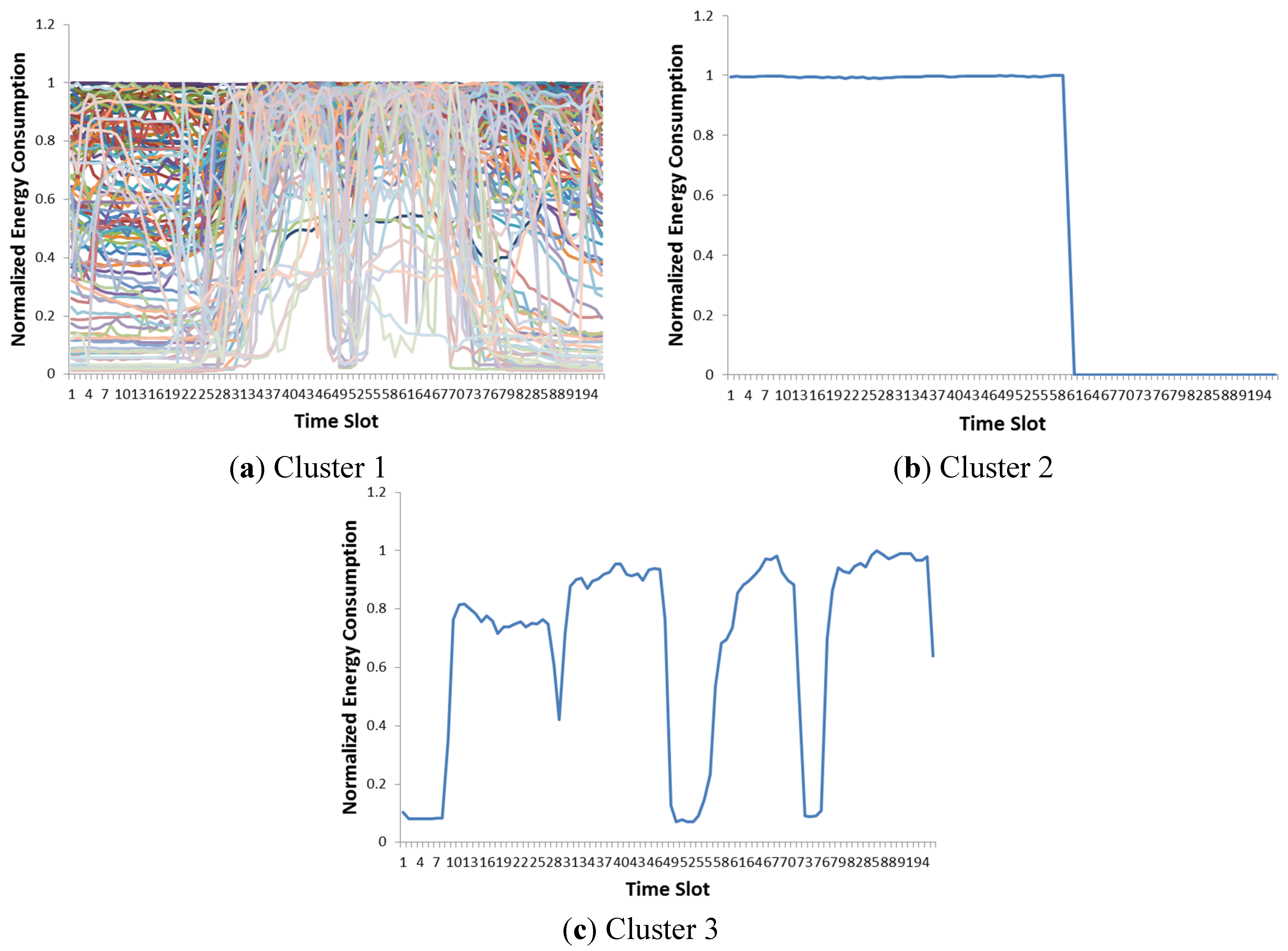
Figure 1 shows an example of customer clusters that we performed with an agglomerative hierarchical clustering method, which is known to produce outstanding clustering results [
7]. The resulting clusters of the hierarchical clustering method consist of a single dominant cluster and many small ones. Despite a promising general cluster performance index from literature [
7], this is definitely not the desired result, as a demand response strategy cannot be designed with these clusters. With various numbers of clusters, unacceptable clusters are still generated. This simple experiment shows the limitation of previous works. Since the previous approaches did not consider the requirements of real applications, cluster results might be meaningless groups of scattered points in a hyperplane. The data used in this analysis are the energy consumption patterns in southern Gyeonggi Province in Korea which are also used in the experiment section.
Figure 1.
Hierarchical clustering result with the single linkage method (number of clusters, k = 3). Hierarchical clustering provides a dominant cluster and other small clusters. (a)–(c) Clusters 1–3.
Figure 1.
Hierarchical clustering result with the single linkage method (number of clusters, k = 3). Hierarchical clustering provides a dominant cluster and other small clusters. (a)–(c) Clusters 1–3.
In this paper, we attempt to develop a clustering method that is applicable to real applications reflecting expert knowledge. More specifically, we propose a good distance measure between customers that fits the customer clustering, especially in demand response applications, based on expert knowledge. This new distance measure, which considers the time-shift characteristic of customers, will be explained and verified in the following sections. Furthermore, we also propose a genetic programming (GP) framework that automatically identifies the clustering principle of the experts. Specifically, we try to derive the ideal distance measure between two customers from expert knowledge using GP.
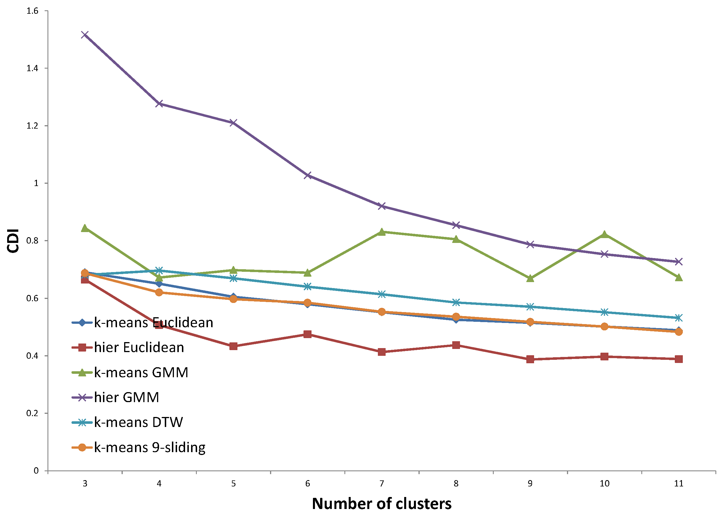
For validation of the clustering results, we do not use traditional performance indexes, such as CDI (Clustering Dispersion Indicator) [
22], VRC (Variance Ratio Criterion) [
23], WCBCR (Ratio of Within Cluster sum of squares to Between Cluster variation) [
20], SI (Scatter Index) [
24], MIA (Mean Index Adequacy) [
22], or DBI (Davies-Bouldin Index) [
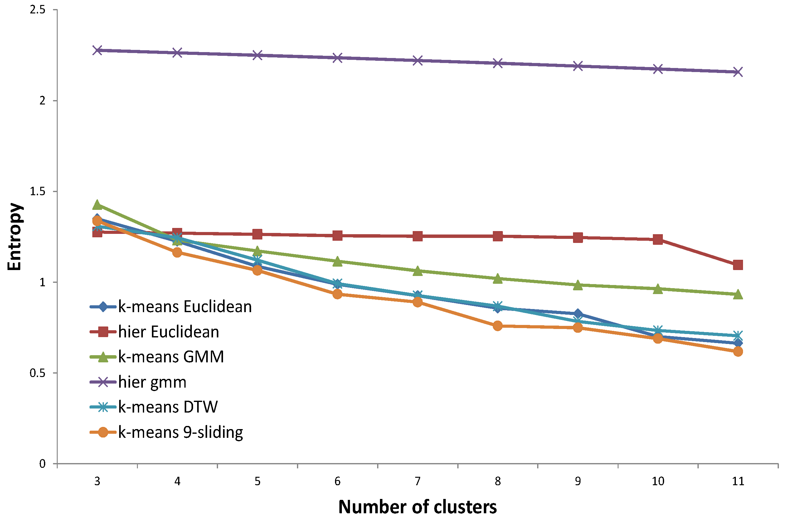
25]. Although these indexes are widely accepted in clustering, they are not proficient in specific applications such as electricity load profile clustering. They do not consider domain knowledge and only focus on the internal structure of nodes. For these reasons, we focus on an external validity index such as entropy, which compares the clustering answer with pre-assigned, ground-truth clusters. Regarding ground-truth clusters, we set up two types of pre-determined clustering answers determined by domain experts and based on the assumption of virtual customers, respectively. The concept of virtual customers will be described in
Section 3.
The contributions of this paper can be summarized as follows.
1. We propose the formation of clusters that are similar to those defined by the experts. The clustering result preferred by experts can be quite different from that generated by most of the clustering methods. To our knowledge, this is the first study to focus on real domain expert knowledge. Furthermore, the problem of inapplicable clustering, shown in
Figure 1, which was the motivation for our study, is presented.
2. The k-sliding distance, which is a new distance measure, is proposed and validated for electricity customer clustering. This distance is designed based on the time-shift characteristic of loads and is designed to produce an improved clustering result, especially in demand response applications. Furthermore, the k-sliding distance can be utilized with any clustering method because it is a distance measure between nodes rather than a clustering method.
3. We propose a GP framework that is formulated to automatically derive the clustering principle of experts. Specifically, we provide an improved distance measure between two customers from expert knowledge using GP. The results with extensive input features show strong support for the proposed k-sliding distance, at least in a demand response application.
The rest of this paper is organized as follows. In
Section 2, a novel
k-sliding distance is proposed. We verified the performance of the
k-sliding distance with extensive experiments in
Section 3. The clustering principle of the demand response experts is analyzed using the GP framework and is validated by experiments in
Section 4 and
Section 5, respectively. The conclusion is presented in
Section 6.
2. k-Sliding Distance
The proposal of this new distance is based on the time-series pattern of electricity consumption data. Most of the previous studies considered these data as a set of independent variables, which is not valid in real applications. Although 96 independent input dimensions in each customer could be a basic approach for clustering, this is not sufficient because they are interrelated in the time domain. The DTW (Dynamic Time Warping) distance, which is specially designed for time-series data, is an attractive candidate and a simple result of electricity customer clustering with the DTW distance is presented by Iglesias and Kastner [
16]. The result, however, only provided the possibility of applying the time-series analysis to electricity customer clustering.
Real electricity applications, especially the demand response application in this paper, have unique viewpoints in defining similarity.
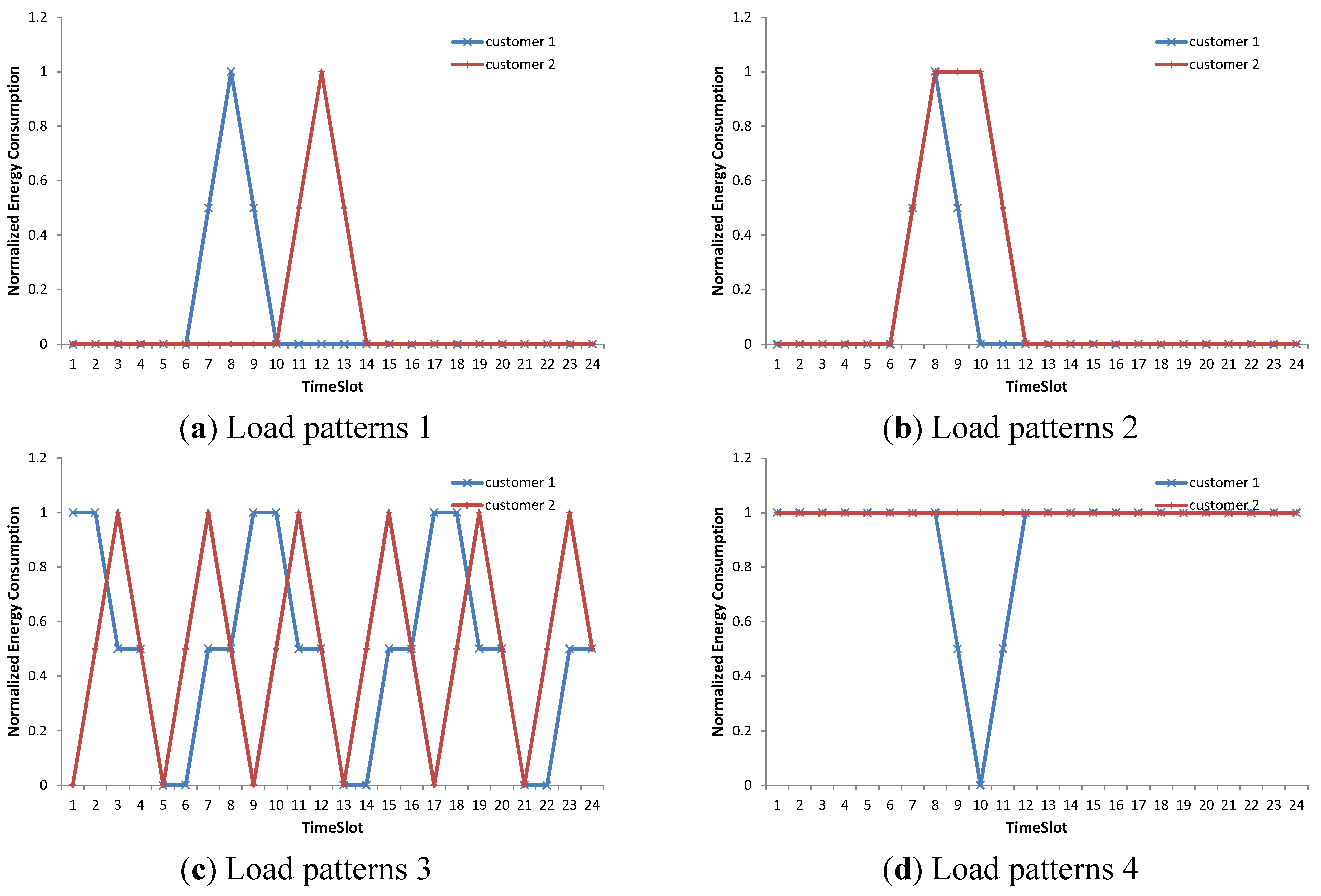
Figure 2, for example, shows a few representative samples that must be considered. In
Figure 2a–c, there are two customers that are assumed to be similar in our demand response application. In
Figure 2a, a small delay in the time dimension can be ignored. Additionally, in
Figure 2b, a small difference in usage duration can be accepted. Two customers, who show similar severe fluctuations, as shown in
Figure 2c, are also expected to be very similar. In contrast, the two customers in
Figure 2d are not similar. Customer #1 can reduce its electricity usage because a sharp drop exists in the pattern. Customer #2 is assumed to be in a different category because it has flat energy usage.
Figure 2.
Representative samples for calculation of similarity. Two customers in (a–c) are considered as they are similar. Customers in (d) are not similar. (a)–(d) Load patterns 1–4.
Figure 2.
Representative samples for calculation of similarity. Two customers in (a–c) are considered as they are similar. Customers in (d) are not similar. (a)–(d) Load patterns 1–4.
It is certain that the Euclidean distance based on the 96 independent dimensions cannot distinguish these characteristics because it does not consider time-related features. For example, by definition, it provides a long distance in the case shown in
Figure 2c.
The k-sliding distance, which we propose here, is an alternative distance measure between two time-series nodes. The definition of the k-sliding distance is presented in Equation (1).
where
is the proposed distance between nodes
i and
j.
is the distance in dimension
d between nodes
i and
j.
The distance between node i and node j is basically the squared sum of the distance in each dimension, which is calculated using Equation (2).
where
k is the sliding limit.
is the energy usage of node
i in dimension
d.
The underlying concept of this distance measure is that time can be shifted to some extent,
i.e.,
k time slots. For example, a peak in electricity usage is allowed to float in the
k time window without any loss of similarity. This is especially important in a demand response application because its focus is on the peak time and load reducibility. We first consider customer
i as a pivot on which to slide the usage pattern of customer
j. The distance in dimension
d is defined as the minimum distance in the
k-sliding window. Because there are two possible pivots, we now have two measured distances in each dimension. The final
k-sliding distance in dimension
d is defined as the maximum of the two measured distances. The reason why we use the maximum of the two distances can be clearly seen in
Figure 2d. If we use customer #2 as the pivot in the 10th time slot, the distance can be zero. If we use customer #1 as the pivot in the 10th time slot, the distance is 1. In the example, we use the larger value as the distance because an asymmetric distance at a certain dimension indicates low similarity.
The difference between the
k-sliding distance and the DTW distance is stated here in order to understand the concept of the
k-sliding distance. The DTW distance only focuses on the well-shaped, time-warping scenario,
i.e., cases
Figure 2a,b. In contrast, the
k-sliding distance can handle complex, mixed scenarios as well as time-warping scenarios. It only focuses on the nearby similar usage values without considering any time-dependent sequences. Simply, the
k-sliding distance looks for nearby points, while the DTW distance looks for matching time sequences.
Table 1 shows the distance measured in the above examples. The Euclidean distance is not acceptable, because it does not consider any time-related aspects. The DTW distance can produce a desirable result only with time-warping scenarios such as those in
Figure 2a,b. In more complex scenarios, such as that in
Figure 2c, DTW generates undesirable results. On the other hand, the
k-sliding distance provides a small value in the cases of
Figure 2a–c and provides a large value in
Figure 2d, which is the expected result.
The k-sliding distance is not a clustering method but a distance measure, like the Mahalanobis distance. Any existing methods such as k-means and hierarchical clustering can be used with the proposed k-sliding distance. Furthermore, the proposed distance can be applied to any consecutive series data, as well as pure power consumption values. For example, the change rate of electricity consumption (i.e., slope of graph) extracted from original data can also be considered as input for the k-sliding distance. Therefore, the proposed distance measure can be easily applicable to other features and can be easily applied to other clustering algorithms.
Table 1.
Measured distances in the example scenarios.
Table 1.
Measured distances in the example scenarios.
| Distance Type | Figure 2a | Figure 2b | Figure 2c | Figure 2d |
|---|
| Euclidean distance | 3 | 1.5 | 6 | 1.5 |
| DTW (Dynamic Time Warping) distance | 0 | 0 | 3 | 3 |
| 4-sliding distance | 0 | 0 | 0.25 | 1.5 |
4. Finding Clustering Principle Using Genetic Programming
In
Section 2 and
Section 3, we proposed and verified a new distance measure that is suitable for demand response applications. Next, we want to know the clustering principles of experts based on the collected data. The principles of clustering can be translated to the definition of the distance measure between two nodes because experts utilize their own combined distance measure. This distance must include many characteristics such as average usage, peak time, and fluctuations. If we know the way to formulate these clustering principles, we can utilize the framework for any application in a smart grid.
More specifically, in this section, we design a GP framework that derives a distance measure from an expert or a group of experts in a demand response application. Although we focus on demand response in this study, this framework can also be applied to other applications. The goal of GP is to produce the distance measure between two nodes that optimizes entropy. The GP technique looks for a tree that represents a distance equation. The tree will automatically evolve to determine the best entropy value with the help of crossover and mutation.
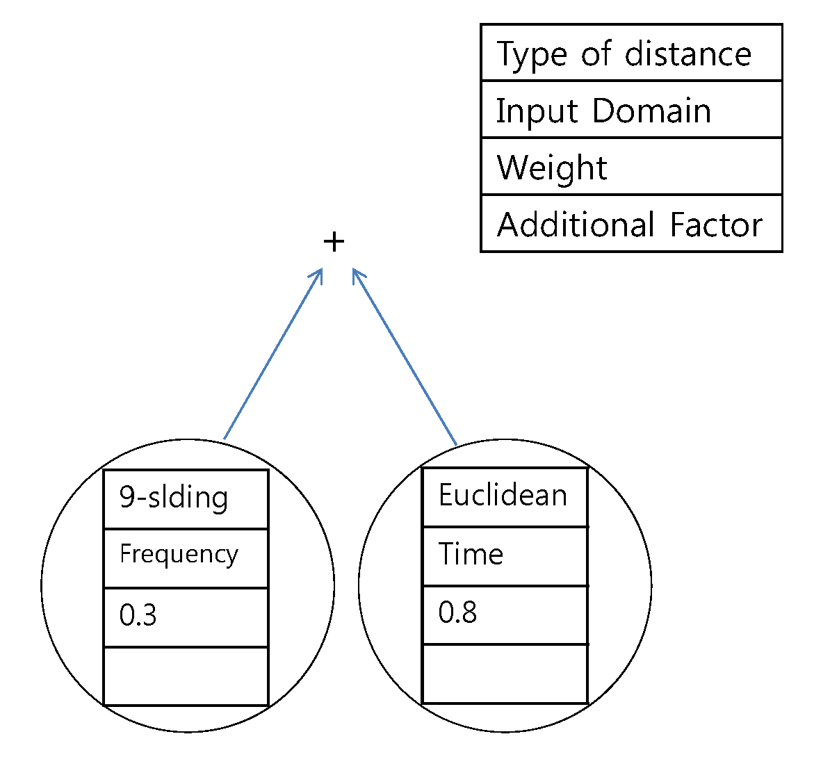
The example tree that is used in this paper is provided in
Figure 14. A leaf node consists of distance options and weights. Examples of distances are the proposed
k-sliding distance and the Euclidean distance. A non-leaf node consists of a binary operator such as summation, subtraction, maximum, and minimum. The generated distance measure shown in
Figure 14 is the sum of the
k-sliding distance in the frequency domain with a weight of 0.3 and the Euclidean distance in the time domain with a weight of 0.8. A total population of 100 and 50 generations are considered in the GP. The depth of the tree was limited to three in order to avoid over-fitting and in order to easily analyze the results. Tournament selection is used as the selection method, and the parameters related to crossover and mutation are applied in an empirical manner. The
k-means algorithm is used for clustering.
Figure 14.
Example tree of genetic programming. The presented distance measure is the sum of the k-sliding distance in the frequency domain with a weight of 0.3 and the Euclidean distance in the time domain with a weight of 0.8.
Figure 14.
Example tree of genetic programming. The presented distance measure is the sum of the k-sliding distance in the frequency domain with a weight of 0.3 and the Euclidean distance in the time domain with a weight of 0.8.
The design of the GP framework is based on the idea that the optimal distance does not consist of a single component. The distance considered by the experts might be the combination of many distances. In order to include various possible distances, we considered input domains such as time, frequency, and slope, as well as distance options such as Euclidean, Pearson correlation, and
k-sliding. Weights and a few additional factors are also included. The parameters of each node in GP are described in
Table 2.
Table 2.
Parameters of nodes in genetic programming.
Table 2.
Parameters of nodes in genetic programming.
| Node Type | Parameters |
|---|
| Leaf (Distance between two customers) | Distance Option | Distance between statistical values, (average, standard deviation), Euclidean distance, DTW distance, Pearson correlation coefficient distance, k-sliding distance |
| Input Domain | Time domain, Frequency domain, Slope domain |
| Weight | 0~1 |
| Additional Factors | Unity operator: sin, cos, square, 1/x, square root, Peak parameter: peak-weight, peak-penalty |
| Non-Leaf | Summation, Subtraction, Maximum, Minimum, Average, Multiplication |
5. Assessment of Distance According to Genetic Programming
Unlike ordinary clustering, both training and test data are needed because the result of the GP must be verified by another test set. This is because GP inherently uses the result in the training phase.
We used two scenarios for verification of the GP framework. The first one is determination of the principle of each expert. In this scenario, both test and training data are generated by the same expert. In other words, the answers of expert #1 for the southern region are input into the GP as training data, and the resulting tree is used as the distance in the k-means clustering for the northern region. As a result, the entropy for the northern region is analyzed. There are four training data sets available, those of two provinces and two experts.
The second scenario is designed to find a common principle of both experts. In this scenario, the answers from both experts #1 and #2 for the southern region are input into the GP as a training set. The resulting tree is used as the distance in the northern region. A scenario using the northern region as a training set is also possible.
Figure 15,
Figure 16,
Figure 17 and
Figure 18, each tree resulting from the first scenario is presented. The first common observation is that none of the trees include the Euclidean distance. This result indicates that people do not see the load pattern in the hyper dimension as does a computer.
Figure 15.
Proposed tree for the southern region using the data of expert #1.
Figure 15.
Proposed tree for the southern region using the data of expert #1.
Figure 16.
Proposed tree for the southern region using the data of expert #2.
Figure 16.
Proposed tree for the southern region using the data of expert #2.
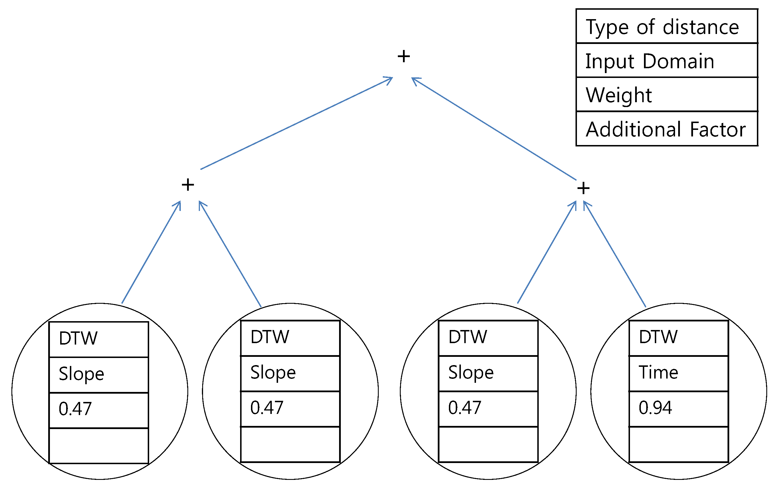
Figure 17.
Proposed tree for the northern region using the data of expert #1.
Figure 17.
Proposed tree for the northern region using the data of expert #1.
Figure 18.
Proposed tree for the northern region using the data of expert #2.
Figure 18.
Proposed tree for the northern region using the data of expert #2.
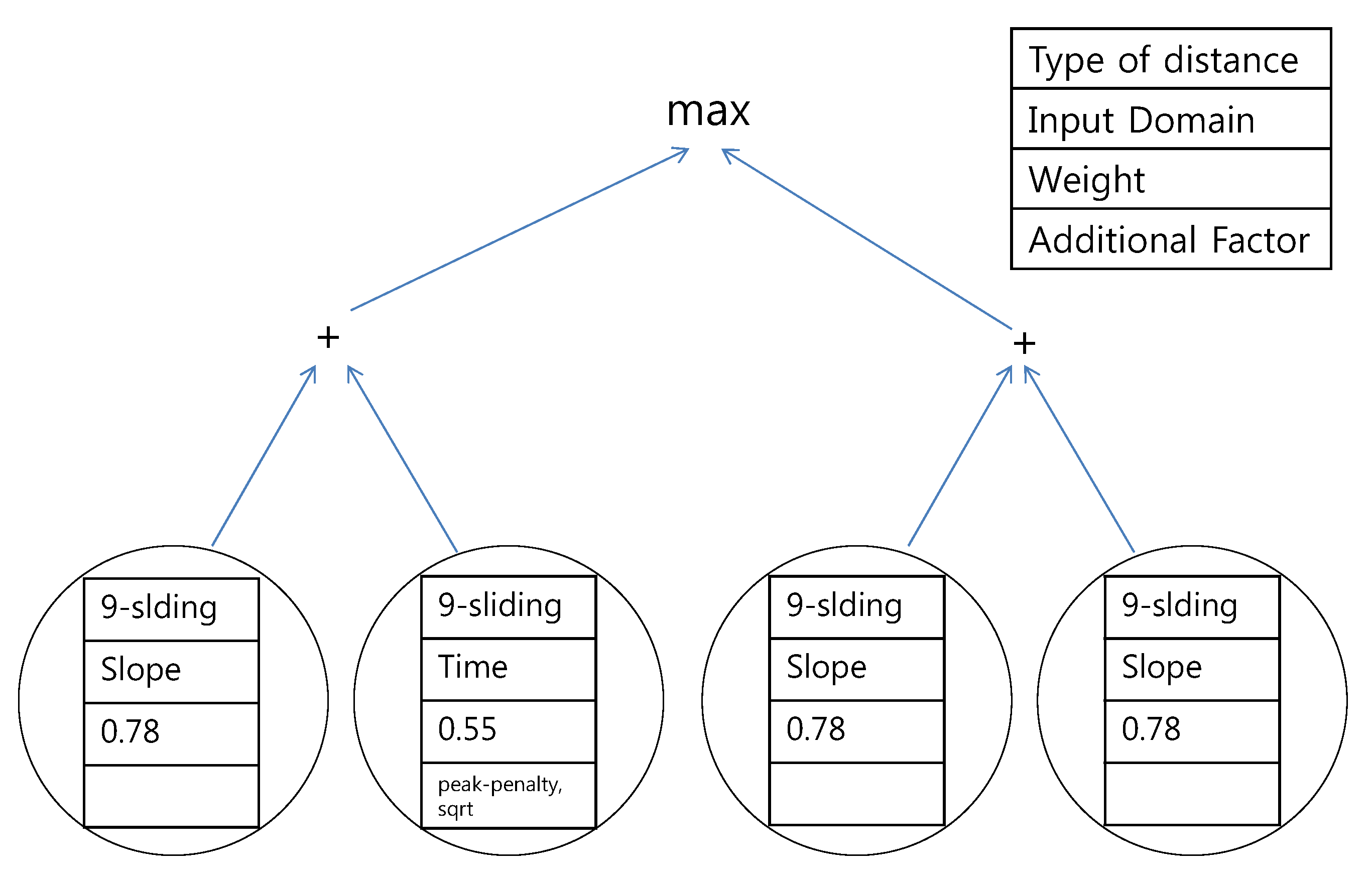
The second observation is that the results are mostly composed of the
k-sliding distance. In most cases (
Figure 15,
Figure 17 and
Figure 18),
k-sliding was the main concern in the tree structure. Exceptionally, DTW is suggested in
Figure 16. The explanation for this is that expert #2 specifically focused on the DTW distance in the southern region.
Another important observation is that the frequency domain input is not utilized at all. The data in time domain was mostly selected by GP. The slope domain, which denotes the sequence of usage differences, also plays a role in the distance selection according to our experiment. From the results, we conclude that the k-sliding distance in the time domain and slope domain is actually meaningful to an expert’s decision.
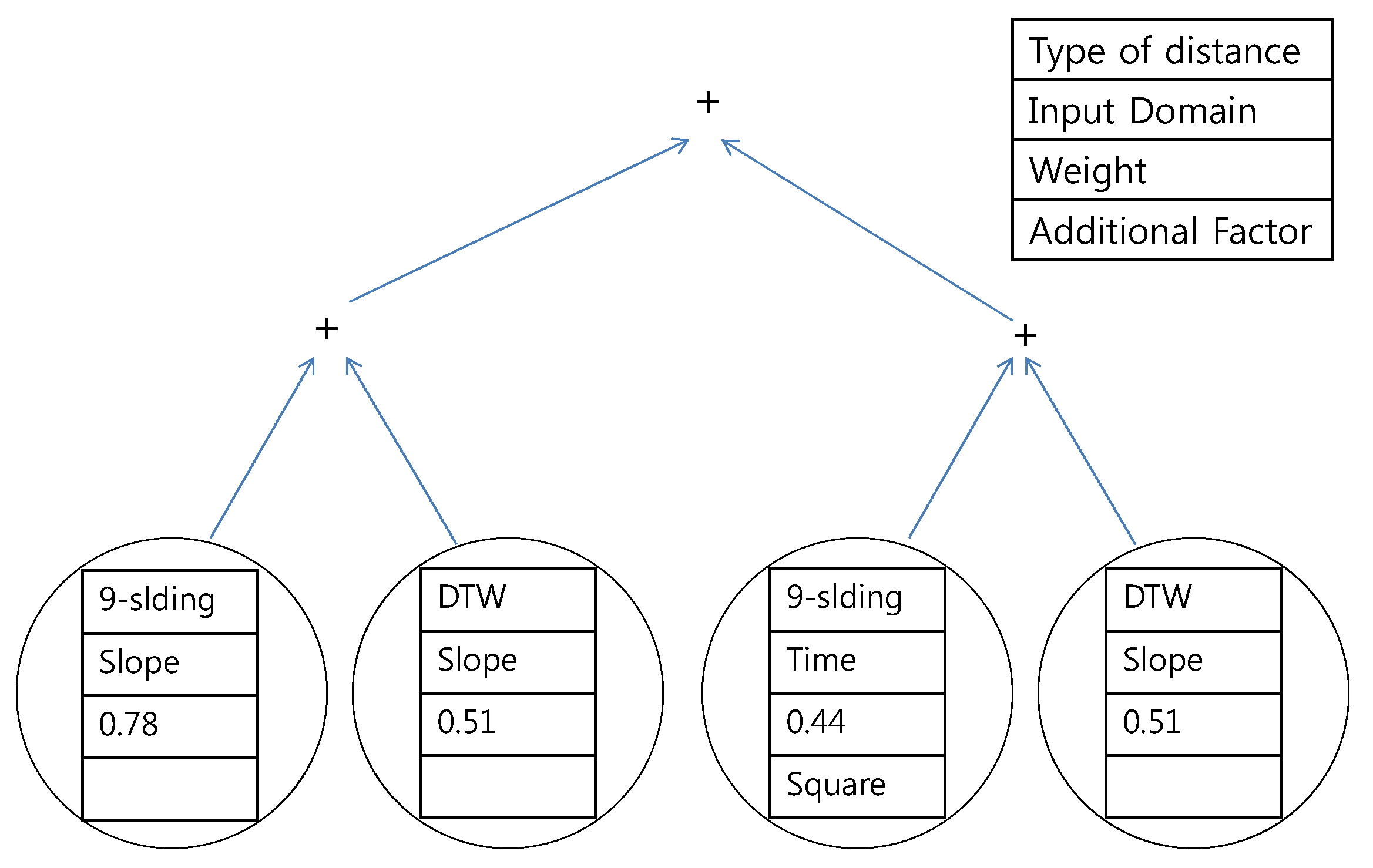
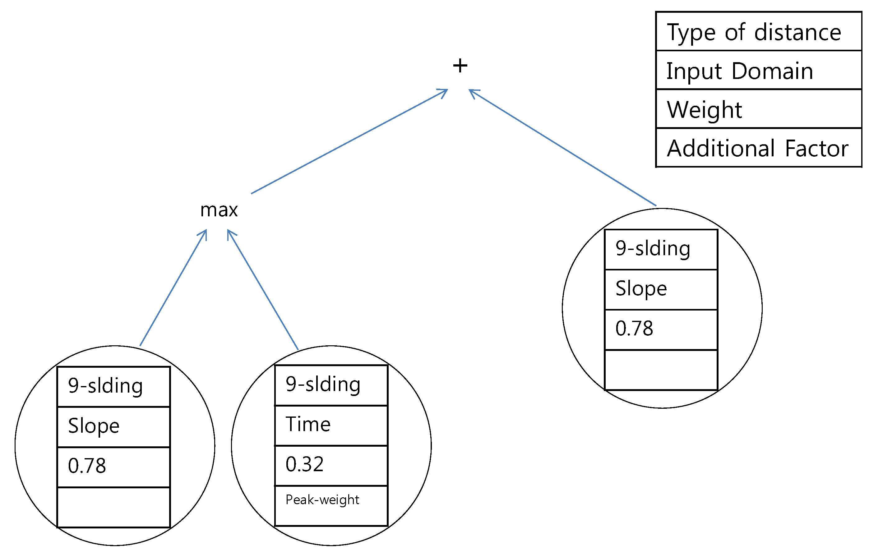
The trees resulting from the second scenario, which looks for the common principles of both experts, are presented in
Figure 19 and
Figure 20. The results are similar to those of the first scenario except that all of the distances are composed of the
k-sliding distance. A combination of the
k-sliding distance in the time domain and the slope domain is generated as the most suitable distance.
Figure 19.
Proposed tree for the southern region using the data of experts #1 and #2.
Figure 19.
Proposed tree for the southern region using the data of experts #1 and #2.
Figure 20.
Proposed tree for the northern region using the data of experts #1 and #2.
Figure 20.
Proposed tree for the northern region using the data of experts #1 and #2.
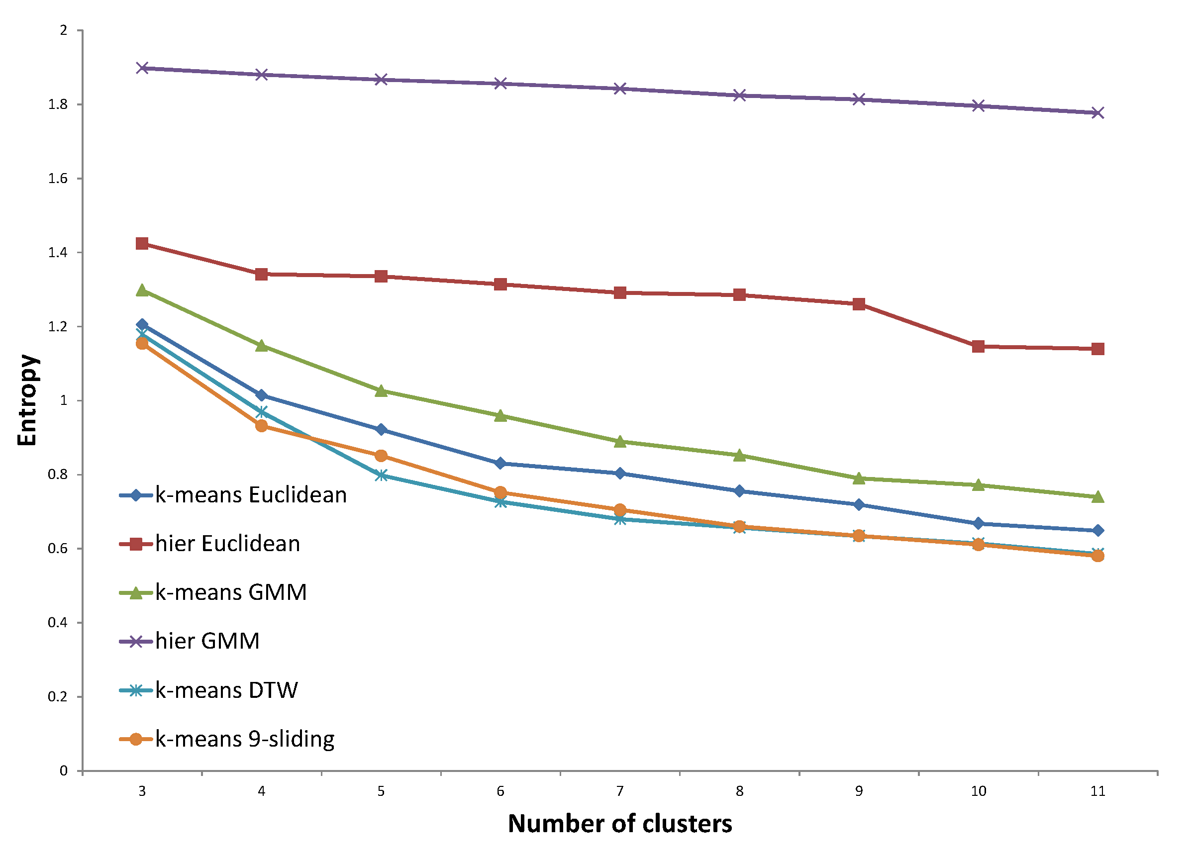
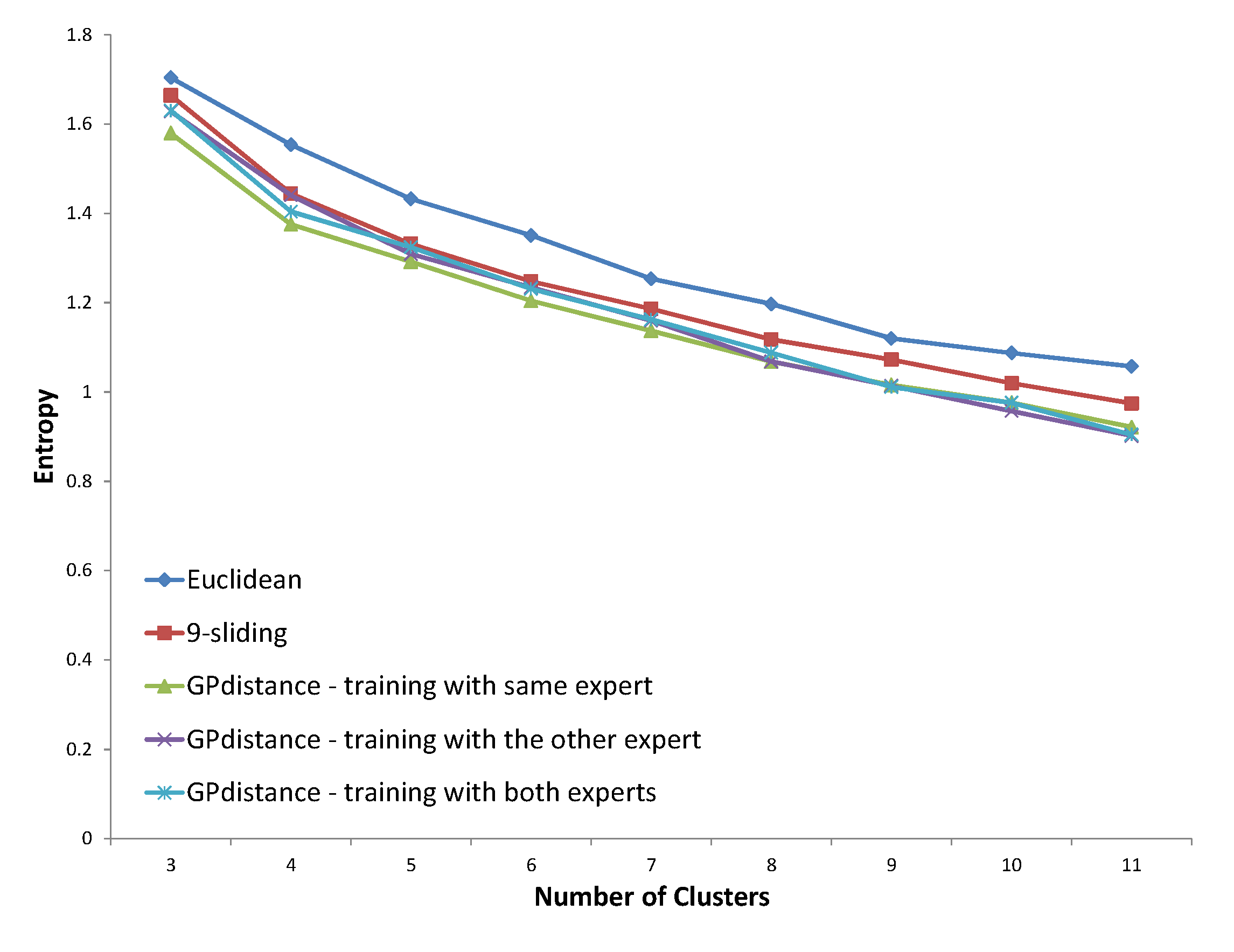
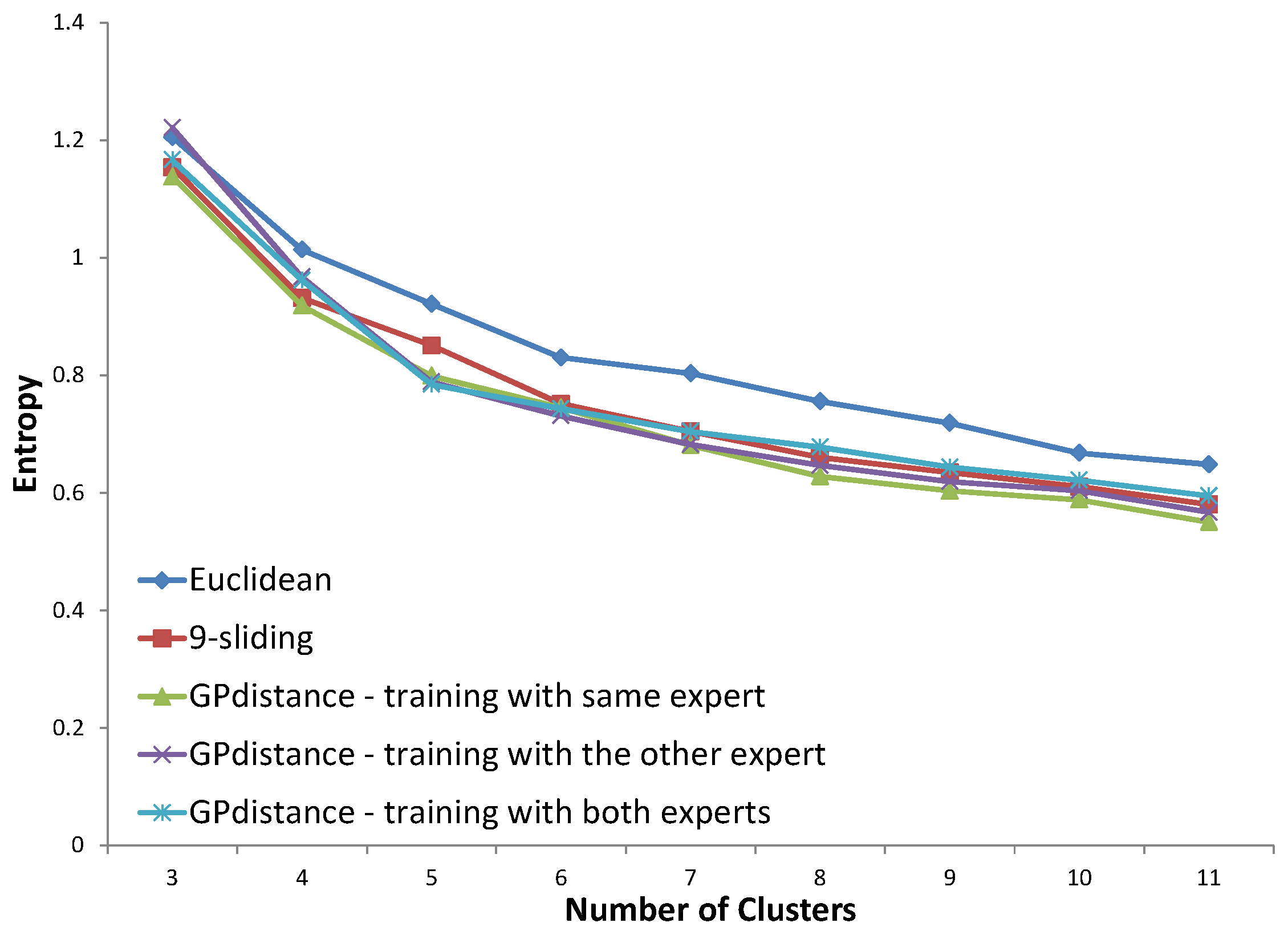
Five distance options are presented in each figure. The Euclidean distance and k-sliding distance are presented as baselines. Three cases are available for GP verification. The first one is the distance that is trained with the same expert’s answer. The second case considers the distance trained with the other expert’s answer. The distance trained with both experts’ answers is considered in the third case. The distance proposed by the same expert’s decision will illustrate the principle of an expert’s clustering decision, and that proposed by both experts’ decisions will illustrate the principle of the expert group. The optimized entropy in the process of GP is not presented here because we need to verify the result on a test set, even though the optimized entropy was much smaller than all other results of the test data.
In
Figure 21, all three distances proposed by the GP provided improved results compared to that of baselines. Specifically, the distance proposed by the same expert’s decision shows consistently lower entropy values. In
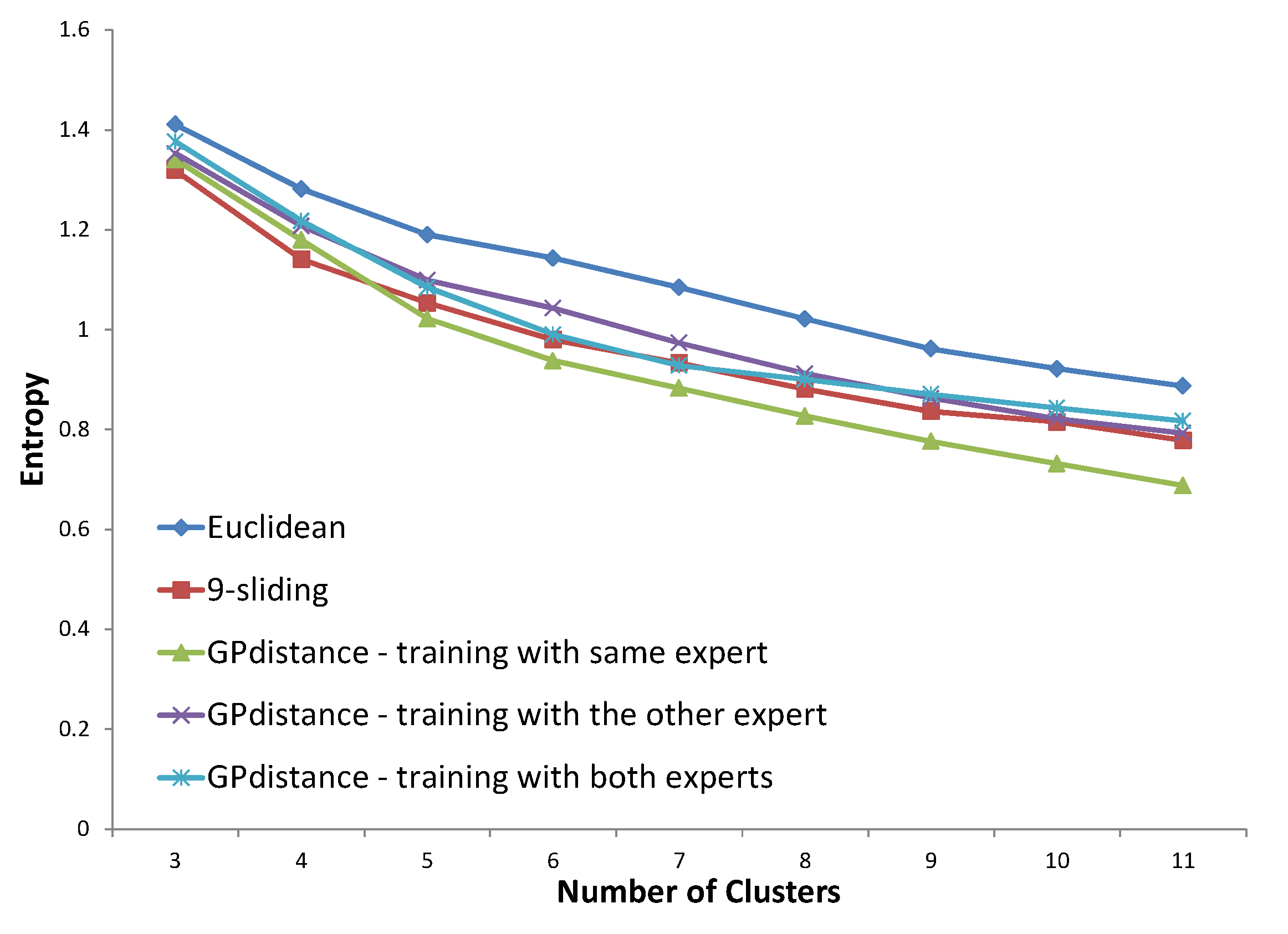
Figure 22, the distance trained with the same expert constantly shows improved entropy results compared to those of the baselines. The distance trained with the other expert shows slightly improved results, while the distance with both experts provides similar results compared to those of the
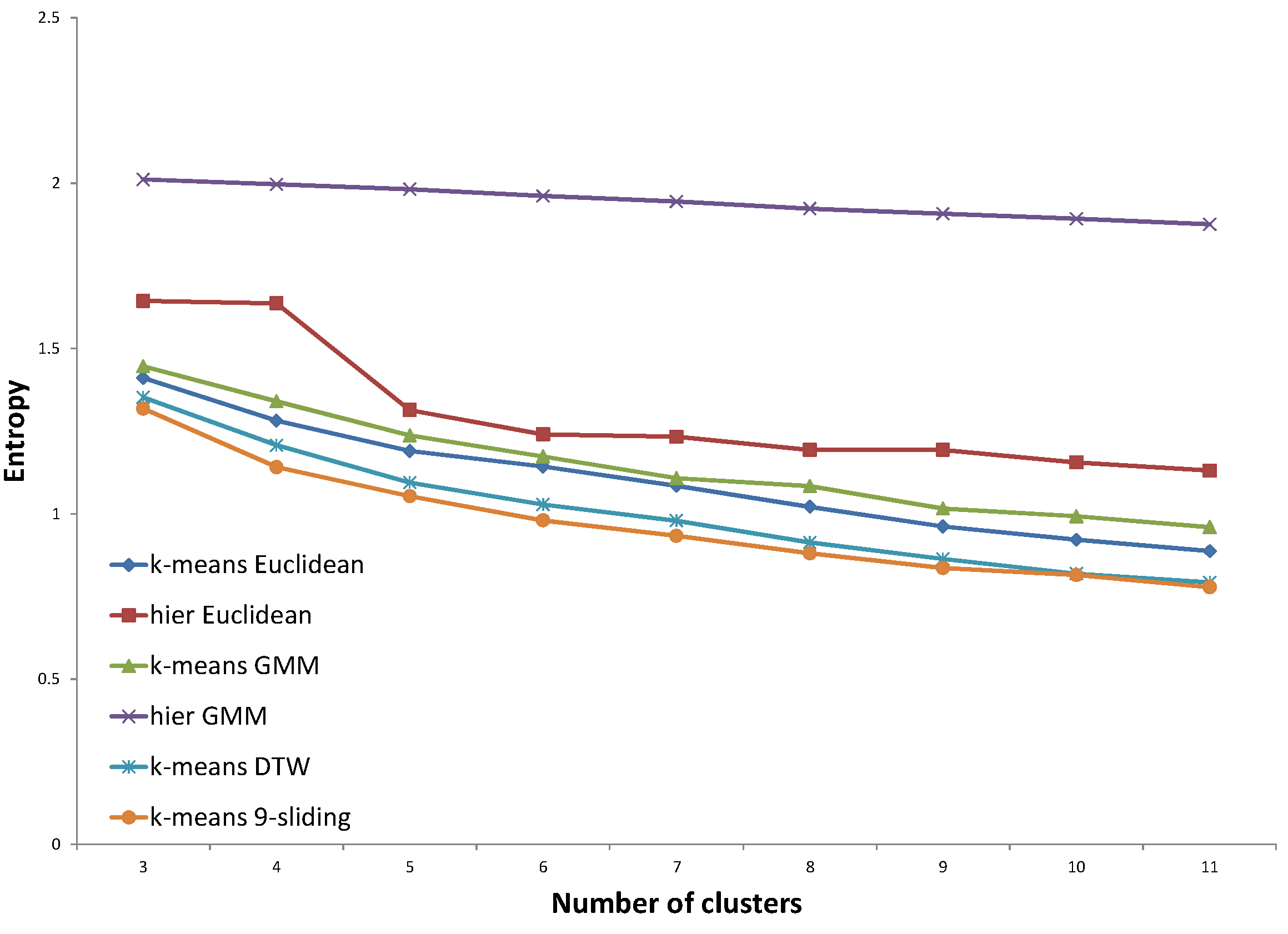
k-sliding distance. In
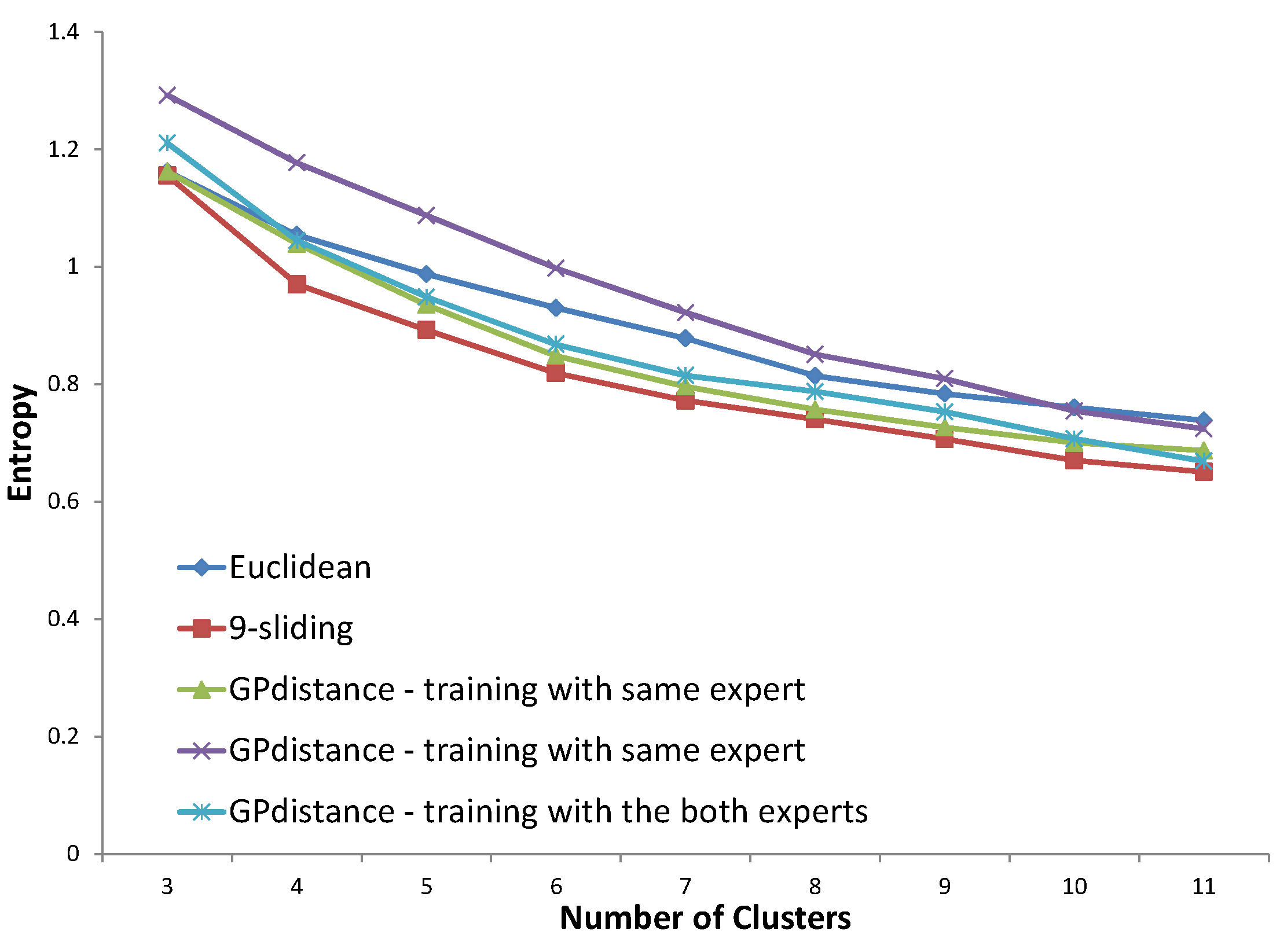
Figure 23, the distance trained with the same expert clearly provides an improved entropy performance, demonstrating 16.1% and 4.7% improvement compared to the Euclidean distance and
k-sliding distance, respectively. The distances with the other expert and both experts, however, provided slightly degraded performances compared to those of the
k-sliding distance.
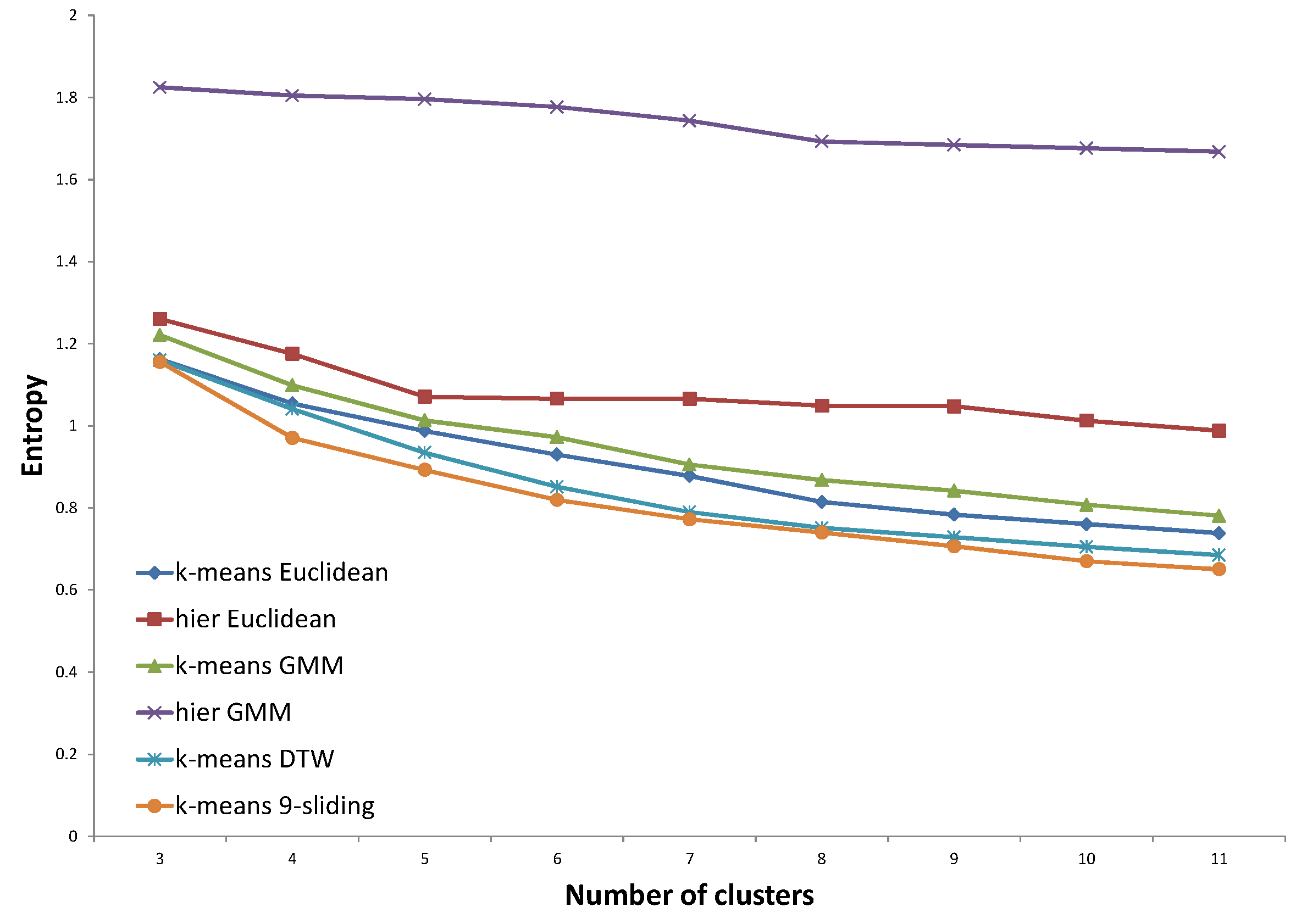
In
Figure 24, for the northern region using the data of expert #2, all three distances determined by GP provided a degraded performance compared to that of
k-sliding. Even the distance trained by the same expert’s answer does not show an improved performance. This exceptional case stems from the fact that the generated distance consists of only DTW distances, according to the tree presented in
Figure 16. The result could be considered to be over-fitting for a special case. This could also happen if the expert’s clustering principle drifts according to the input data set. Either way, from this result, we conjecture that expert #2 has a relatively fluctuating principle compared to expert #1.
Figure 21.
Entropy results for the southern region using the data of expert #1.
Figure 21.
Entropy results for the southern region using the data of expert #1.
Figure 22.
Entropy results for the southern region using the data of expert #2.
Figure 22.
Entropy results for the southern region using the data of expert #2.
Figure 23.
Entropy result for northern region using the data of expert #1.
Figure 23.
Entropy result for northern region using the data of expert #1.
Figure 24.
Entropy results for the northern region using the data of expert #2.
Figure 24.
Entropy results for the northern region using the data of expert #2.
Despite the exceptional results shown in
Figure 24, the average improvement in GP distance trained with the same expert was 11.2% compared to the Euclidean distance and 2.2% compared to the
k-sliding distance. When we required the use of at least seven clusters, the improvement increased to 13.3% and 3.4% compared to the Euclidean distance and
k-sliding distance, respectively. This means that too few clusters cause an erroneous result because the number of clusters determined by experts is approximately 10. Based on the results, we conclude that the GP can clearly identify the clustering principle of an expert.
The average improvement in GP distance that is trained with both experts’ answers was 8.7% and −1.5% compared to the Euclidean distance and
k-sliding distance, respectively. The clustering principle of the two joint experts was also found because it provides an improved result compared to the Euclidean distance. The entropy, however, is not improved compared to the
k-sliding distance. There are two possible reasons for this result. The first is that the generated distance mainly consists of the
k-sliding distance (
Figure 19 and
Figure 20). Because the component of the proposed distance is the
k-sliding distance, a considerably improved result cannot be expected when we compare it to the
k-sliding distance. The second reason is that the two experts have slightly different clustering principles according to their individual knowledge. This is verified by the fact that the distance trained with the other expert’s answer usually does not provide decreased entropy (
Figure 22,
Figure 23 and
Figure 24).
From the results, we conclude that the clustering principle can be derived from a single expert. This, however, does not imply that the clustering principle of a group of experts cannot be derived. Actually, the results show that a clustering principle actually exists for a certain expert. We expect that a more sophisticated derivation of the clustering principle can be determined for a group of experts, even though the result was not improved compared to that of the proposed k-sliding distance in our experiment due to a small number of experts.
In summary, in all cases involving two provinces and two experts, the principle found with the GP was mainly composed of the k-sliding distance and DTW distance in the time domain and slope domain. The result of the GP showed the possibility of finding clustering principles because it showed an improved result compared to the Euclidean distance in all of the cases and compared to the proposed k-sliding distance in most of the cases.


