

The Electrical Conductivity of Ionic Liquids: Numerical and Analytical Machine Learning Approaches


Condensed Matter Physics Laboratory, Department of Physics, University of Thessaly, 35100 Lamia, Greece
*
Author to whom correspondence should be addressed.
Fluids 2022, 7(10), 321; https://doi.org/10.3390/fluids7100321
Submission received: 3 September 2022
/
Revised: 27 September 2022
/
Accepted: 28 September 2022
/
Published: 5 October 2022
(This article belongs to the Special Issue Machine Learning and Artificial Intelligence in Fluid Mechanics)
Abstract
:In this paper, we incorporate experimental measurements from high-quality databases to construct a machine learning model that is capable of reproducing and predicting the properties of ionic liquids, such as electrical conductivity. Empirical relations traditionally determine the electrical conductivity with the temperature as the main component, and investigations only focus on specific ionic liquids every time. In addition to this, our proposed method takes into account environmental conditions, such as temperature and pressure, and supports generalization by further considering the liquid atomic weight in the prediction procedure. The electrical conductivity parameter is extracted through both numerical machine learning methods and symbolic regression, which provides an analytical equation with the aid of genetic programming techniques. The suggested platform is capable of providing either a fast, numerical prediction mechanism or an analytical expression, both purely data-driven, that can be generalized and exploited in similar property prediction projects, overcoming expensive experimental procedures and computationally intensive molecular simulations.
1. Introduction
The investigation of complex materials has raised ever-growing interest among researchers in the area of fluid mechanics. Following an in-depth understanding of the internal atomic/molecular structure and the physics behind the imposed interaction mechanisms, advanced simulation techniques and experimental procedures are incorporated in order to extract the fluid properties and open the road to advances in the manufacturing and controlling of novel devices. The numerical modeling of such processes has always been an efficient, fast, and accurate choice for addressing these objectives, posing as the alternative to complex, time-consuming, and costly experiments. Among the proposed computational methods, machine learning (ML) techniques have now become a standard, showing remarkable efficiency, reduced processing time, and accuracy [1,2].
The existence of a certain number of data in a reliable database is a prerequisite for the adoption of ML. Data-driven approaches have been exploited to deal with complex physical processes, which are not described by analytical expressions and are mostly difficult to measure [3]. In most studies, the research data are obtained via limited experimental conditions. For fluid and material research, experimental results may not be sufficient to meet the ML demands, limiting its further development. Even when the research data are enriched with simulation results, and therefore sufficient, there may also be inherent processing difficulties because of the large number of input features to extract the desired prediction [4]. Therefore, high-quality training data production [5], along with ML adoption complimentary to simulation and experiments [6], can progress material discovery and investigation.
In material science and engineering, the field of application is enormous. Imaging data from microscopic studies and advanced informatic tools have been exploited for material characterization [7], and images from molecular dynamic (MD) simulations have been used to predict ice nucleation from ambient water [8]. The construction of potential energy surfaces (PESs), which had traditionally been a demanding ab initio simulation task, has been boosted by the Gaussian process regression (GPR) methods [9,10]. ML has also been successfully incorporated for the prediction of behavior from data in the fields of biological, biomedical, and behavioral sciences [11]. Fluid research has much to profit from reduced order models, turbulence modeling, fluid property extraction, and potential map creation with ab initio accuracy [12,13].
All these applications are only a small percentage of the true potential data science and ML have to offer. The new research directions focus on integrating physics-oriented parameters and domain knowledge with the proposed ML models. Physics-informed techniques have been suggested, integrating the knowledge of fundamental physics inside an algorithmic procedure [14]. Moreover, as a step toward explainable and generalizable ML, the method of symbolic regression (SR) has evolved, providing not only accurate predictions but also, more significantly, mathematical expressions that describe the phenomena under investigation, beyond classical regression methods [15,16].
In this paper, ML is approached from the perspective of ionic liquids (IL), a class of solvents that have lately attracted increasing attention due to their unique properties. Their important feature is that the melting point is so low that they remain liquid at ambient temperature, while common salts are usually solid at ambient temperature and melt at several hundred degrees Celsius [17]. Their other characteristic properties include negligible vapor pressure, high thermal and chemical stability, high ion conductivity, and nonflammability [18]. IL properties might as well be tuned for a specific application by the proper manipulation of anions and cations, from catalysis and electrochemistry to liquid crystal development, fuel production, and as electrolytes in lithium batteries, supercapacitors, and fuel cells [19]. ILs may serve as unique solvents in electrochemical processes where the use of water is forbidden [20], such as in electroplating and the electrodeposition of metals. Moreover, they are capable of dissolving organic compounds of great biological and ecological importance, such as enzymes, proteins, and cellulose [21].
The experimental measurements of ILs’ physical quantities, such as conductivity, viscosity, and density, as a function of temperature or pressure, are usually performed with optofluidic and microscopic techniques [22,23], and empirical relations have been drawn to guide the experiments [24]. On the other hand, research efforts on property calculation have been mainly based on trial-and-error methods to bind anions and cations to constitute an IL of desired properties. Computational property estimation can bring research to the next level through the incorporation of novel ML methods [25]. Recent studies refer to ML techniques for ILS property prediction, such as viscosity and electrical conductivity [26], CO2 capture capability [27], density, heat capacity, and thermal conductivity [28], among others, trying to depict the relationship between property and molecular structure, and environmental conditions.
Next, we present ML data-driven methods to extract the electrical conductivity, σ, of ionic liquids, both in numerical and analytical form. The incorporated data and pre-processing methods are presented, the ML techniques are described, and the validity of the predictions is discussed. We conclude that the proposed ML-based method is able to reproduce the electrical conductivity values for complex ILs, taking into account the environmental conditions (temperature and pressure) and the molecular weight of the IL of interest. To our knowledge, there has not been another numerical or analytical method able to extract IL properties from these three input parameters, and it can provide a fast and efficient choice to replace/complement timely and costly experiments, especially when the experimental conditions are extreme.
2. Materials and Methods
2.1. The Electrical Conductivity of Ionic Liquids
The physical properties of ILs, such as viscosity, conductivity, and density, are vital for the characterization of salt as being appropriate for a given application or not [29]. The electrical conductivity of ILs is primarily important for the understanding of their behavior and the applications that may profit from tuning their value. ILs can remain at a liquid state for a wide range of temperatures, and many electrochemical applications would incorporate them as solvents. Thus, it becomes clear that there is a need to define the possible parameters that affect electrical conductivity. In most of the studies in the literature, the temperature is the only parameter taken into account and is usually analyzed through the Vogel–Fulcher–Tammann (VFT) curves on the measured data [30,31]. The empirical VFT equation is given by
which is also examined in its linear form as
where the maximum conductivity is , and the activation energy for conduction is = , where is the Boltzmann constant, both of which are derived from fitting the experimental measurements [32], and T0 is the Vogel temperature.
Another empirical relation connects σ with the molecular volume , i.e., the sum of ionic volumes of the constituent ions as [33].
where c and d are the empirical constants of the best fit on the experimental data, while approaches that replace experimental measurements with computational models have been also proposed [34].
2.2. Electrical Conductivity Data
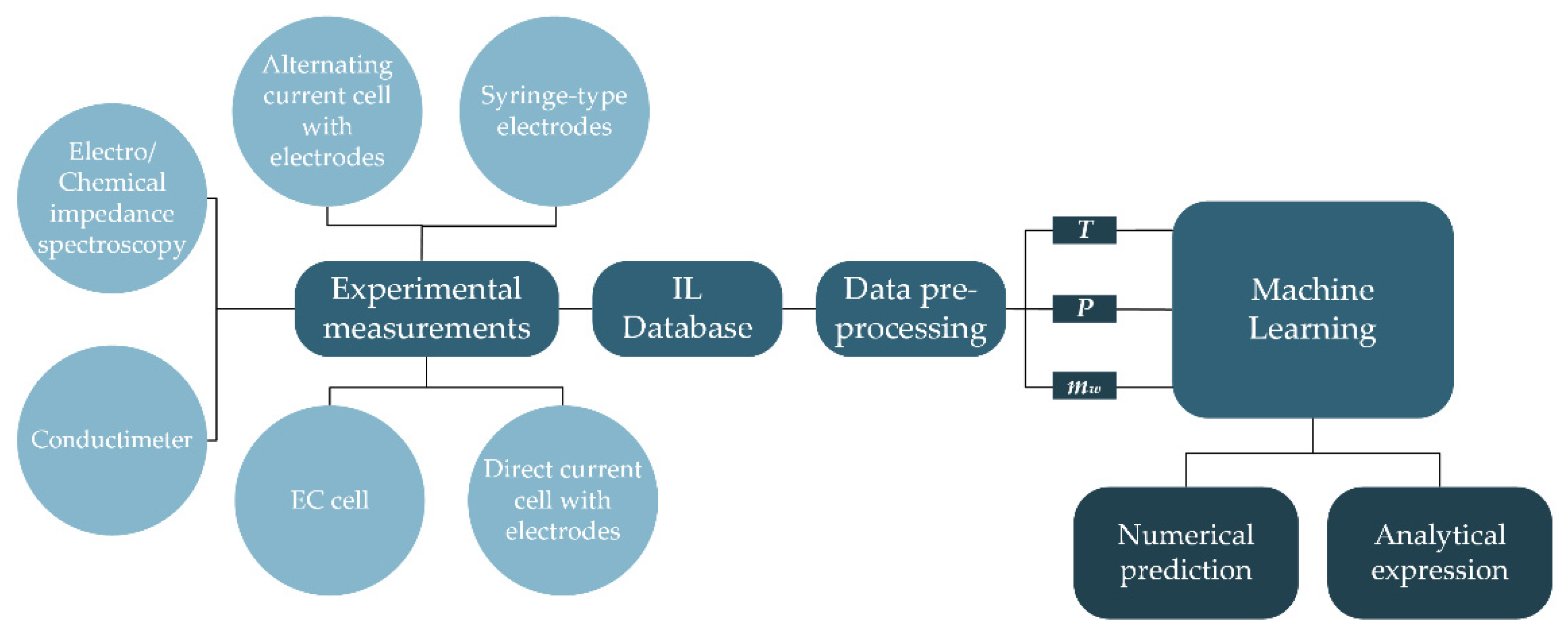
For the computational model adopted in this paper, we followed the steps shown in the flowchart in Figure 1. The modeling started with database creation. High-quality experimental data (2274 points) from the NIST IL-Thermo database [35,36] were gathered for pure ionic liquids, with electrical conductivity being the property of interest. The parameters that affect electrical conductivity, as shown from the experiments, are the temperature, T, the pressure, P, and the liquid molecular weight, Mw. Table S1 (see Supplementary Material File S1) presents all the details for data origin and characteristics, while the IL database is provided in Supplementary Material File S2. The details on the incorporated experimental methods can be found in the respective references [32,37,38,39,40,41,42,43,44,45,46,47,48,49,50,51,52,53,54,55,56,57,58,59,60].
2.3. Pre-Processing
It is common practice before entering the ML procedure, that data are normalized to restrict the input value range.
A correlation check was also performed in order to ensure that the input variables are not correlated to each other, and Figure 2 presents the correlation matrix. It is shown that no kind of correlation existed between the inputs, while the output was mostly correlated to temperature, T.
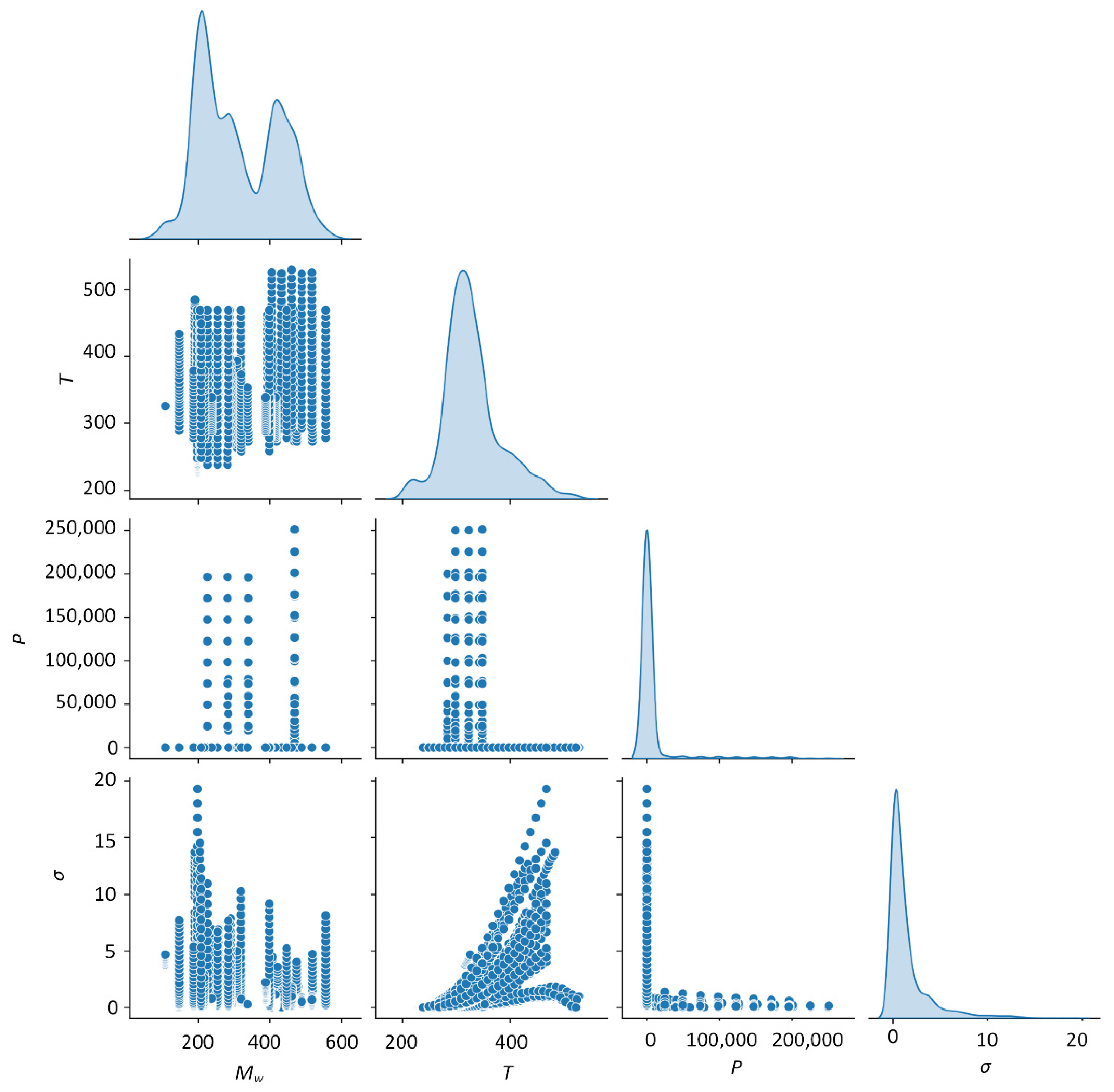
The statistical information for the input data can be obtained from the pair plot diagram in Figure 3. The distribution of the three input parameters, T, P, and Mw, and the output, σ, is shown. The investigated ionic liquid is distinguished by the value of the molecular weight, which, in this paper, ranged from . The temperature and pressure conditions were , and , respectively. The output was in the range of .
2.4. Machine Learning
A supervised machine learning algorithm accepts a number of input data, is trained by a percentage of the data, and enters a computational process to extract the predicted values for the model’s output(s) [61]. Data quality and quantity are important factors here. When representative data (uniformly distributed) existed, and their number was adequate to train the algorithm, the predicted output was obtained, as long as the incorporated algorithm was able to capture their behavior. The verification of the result was made by the remaining part of the input dataset (testing set). The training/testing set percentage on the total data points was taken here as 80/20.
Here, we incorporated six different numerical ML algorithms, namely the multiple linear regression (MLR), k-nearest neighbor (KNN), decision tree (DT), random forest (RF), gradient boosting regressor (GBR), and multi-layer perceptron (MLP) models, to propose the one that provided the best fit to our experimental data. These were implemented with aid of the respective functions from the sci-kit learn Python package [62]. Moreover, the symbolic regression (SR) algorithm was constructed and adjusted from a Julia package [63], in order to provide an analytical expression exclusively extracted from the data and generalizable to electrical conductivity predictions for all input cases, even those outside the data range.
2.4.1. Multiple Linear Regression
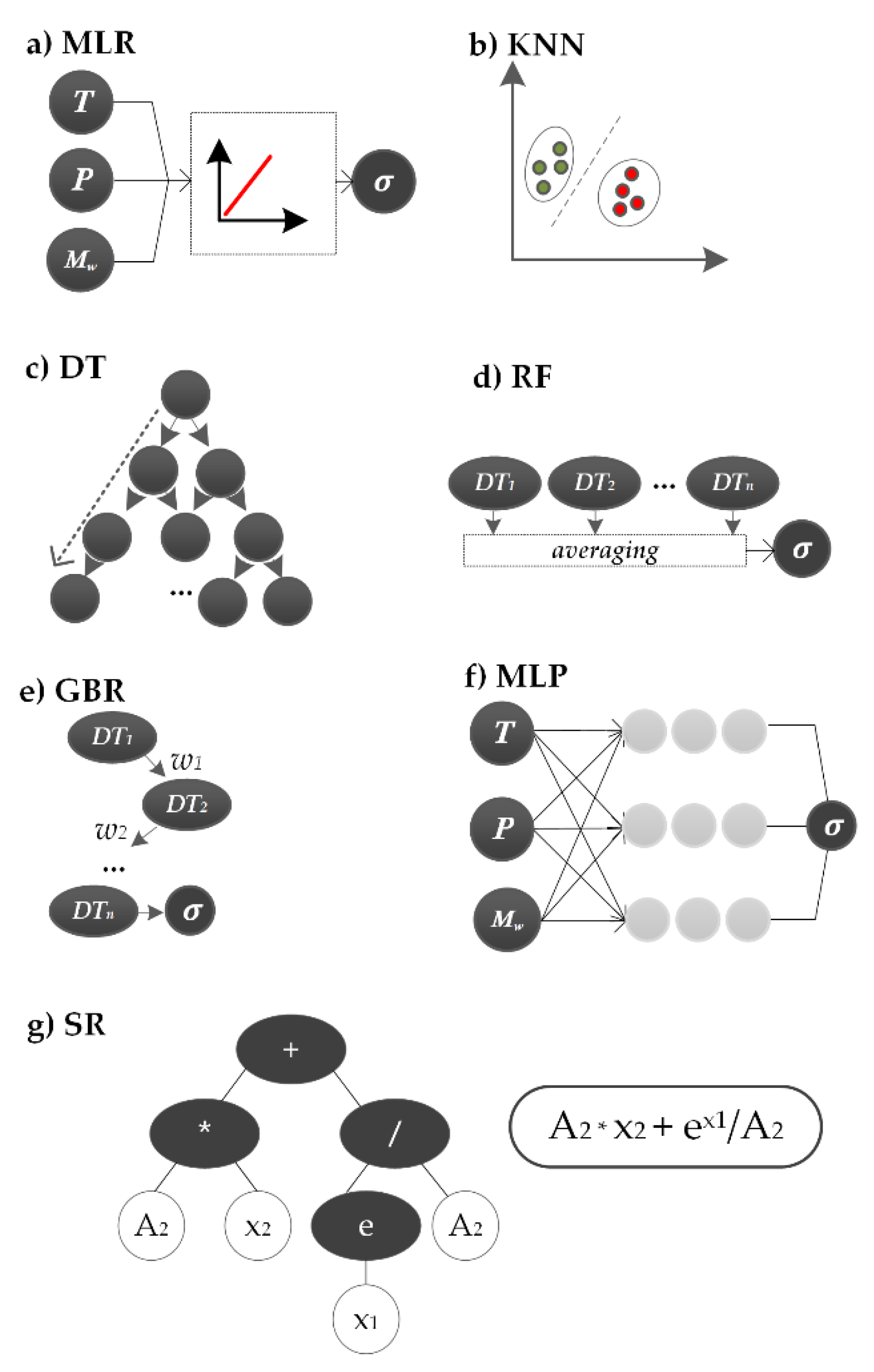
Regression analysis refers to either a univariate method to analyze the relationship between a dependent variable and one independent variable or a model with one dependent variable and more than one independent variable, in which case it is called multiple linear regression (MLR) [64]. In MLR (Figure 4a), we consider n independent input variables, linearly combined to extract the dependent variable as
where are the weights imposed on the three respective inputs , and is a bias term.
2.4.2. k-Nearest Neighbors
The k-nearest neighbor (k-NN) algorithm selects k training points over a local region of a data point x and labels neighboring points on the basis of the Euclidean distance (Figure 4b). Each sample is a pair including an input vector and the desired output. After grouping the calculated distances from the lowest to the highest, the most prevalent outcome from the first k rows is the predicted result [65]. This algorithm is oftentimes accurate; however, there are cases where it may result in slow execution speed and large memory requirements [66].
2.4.3. Decision Trees
The decision tree (DT) algorithm functions in the sense of a tree flowchart, with nodes, branches, and leaves. Each node represents a test on a feature, and each branch represents the result of that test [67]. The DT mo’el’s response is predicted by following the decisions from the start to the end node (the leaf), as shown by the dotted line in Figure 4c. The feature space is recursively partitioned based on the splitting attribute. Each final region is assigned a value to estimate the target output. The DT algorithm is considered easy to apply, although it might need contribution from other statistical methods to prevent overfitting [68].
2.4.4. Random Forest
A random forest (RF) algorithm consists of various DTs working in parallel (Figure 4d). Each tree outputs a different prediction, and their average is taken as the final prediction. Higher accuracy is usually obtained when the number of trees in the forest increase. In the literature, it has been shown that the random forest (RF) algorithm is much simpler to implement, than complex neural network structures, and has been the most accurate choice for fluid applications, such as slip length estimation [69] and the extraction of fluid transport properties [12,70]. All the trees’ outputs are averaged (b is the trees’ number) by
providing an even more accurate result than the single-tree structure, hence less prone to overfitting.
2.4.5. Gradient Boosting Regressor
The gradient boosting regressor (GBR) algorithm is another implementation of a decision tree algorithm that combines various simple functions (learners) that constitute an ensemble function. Initial learners may be weak, but when combined, they may form strong learners. GBR follows three main steps sequentially: It optimizes the loss function, spots the weaker learner, and improves it by adding more trees to increase accuracy [71]. As shown in Figure 4e, the sequential DTs were incorporated, and the output of each one was weighted to enter the next DT. The weights were selected in a way to minimize the induced errors [72].
2.4.6. Multi-Layer Perceptron
The traditional perceptron, when presented in multiple layers, i.e., the input, the output, and a number of internal hidden layers, constitute the multi-layer perceptron (MLP) algorithm. The number of hidden layers is usually determined by trial and error, although there have also been various methods proposed, such as genetic programming [73]. Here, we considered three hidden layers, each one with 20 nodes, with Adam stochastic solver [74] and a learning rate equal to 0.5 (Figure 4f). The data flow between neurons depends on the activation functions applied in every internal node and a weight function imposed on every input. These weights are adjusted so that the predicted output resembles the expected output with minimum error. The training of the MLP was performed iteratively, with backward computation capability.
2.4.7. Symbolic Regression
SR can also be represented by tree structures (Figure 4g); however, here, the tree nodes are mathematical operators, and leaf nodes correspond to input variables/constants [75]. The algorithm begins by considering a random parent tree structure, calculates the mean squared error (MSE) of the specific implementation, and follows an iterative procedure, in which a node or a branch of nodes is substituted until the minimum MSE is achieved, with low complexity. Complexity refers to the number of leaves and nodes used in the proposed SR tree. The Julia-based SR algorithm by Cranmer et al. [63], which we have widely incorporated in similar works [16,76], accepts a set of mathematical operators and the input variables and creates an equation pool, from which it selects the best candidates that adhere to the Pareto front, i.e., those that present the minimum MSE values and small complexity, along with physical correspondence to the problem.
Although more computationally intensive and demanding, SR is capable of providing an analytical expression at hand, which, if it fits the dataset under investigation, is superior to other ML techniques, since it can be easily applied for a wide range of inputs. However, care has to be taken so that this expression remains simple and is bound to physical laws [76].
2.4.8. Metrics of Accuracy
A number of popular metrics were applied to every algorithmic result to determine which one best satisfies the accuracy criteria. These were the coefficient of determination, R2, the mean absolute error (MAE), the mean squared error (MSE), and the average absolute deviation (AAD) [77], as shown in Equations (7)–(10):
with the mean value of the expected output:
where and .
3. Results and Discussion
3.1. Partial Dependence
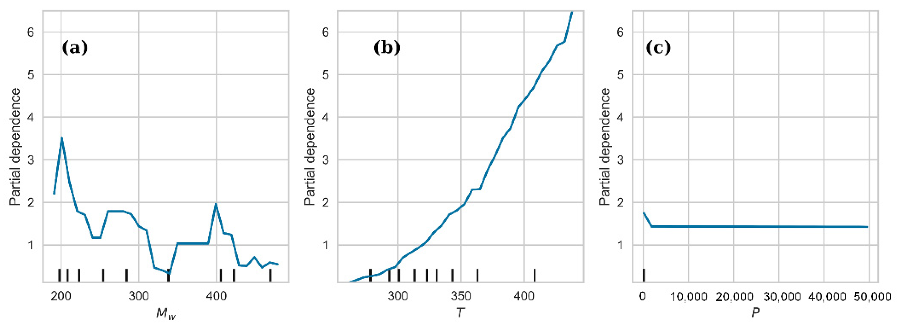
To analyze the effect of each input parameter on the acquired electrical conductivity value, σ, a partial dependence plot was constructed (Figure 5). The partial dependence plot calculates the average marginal effect on the σ prediction when only one input variable changes its value, and, in parallel, the remaining inputs remain constant. The estimation of the partial dependence (normalized value) is shown on the vertical axis and the respective input on the horizontal axis. In Figure 5a, it is observed that the molecular weight significantly affected σ, especially on smaller values around 200–230. The effect of temperature was prominent, especially for the values above 270 K (Figure 5b). On the other hand, pressure had only a slight, inversely linear effect on σ for small pressure values, since partial dependence decreased as the pressure increased (Figure 5c). Furthermore, it seems that σ was practically unaffected by P for the values above 100 kPa.
3.2. Machine Learning Results
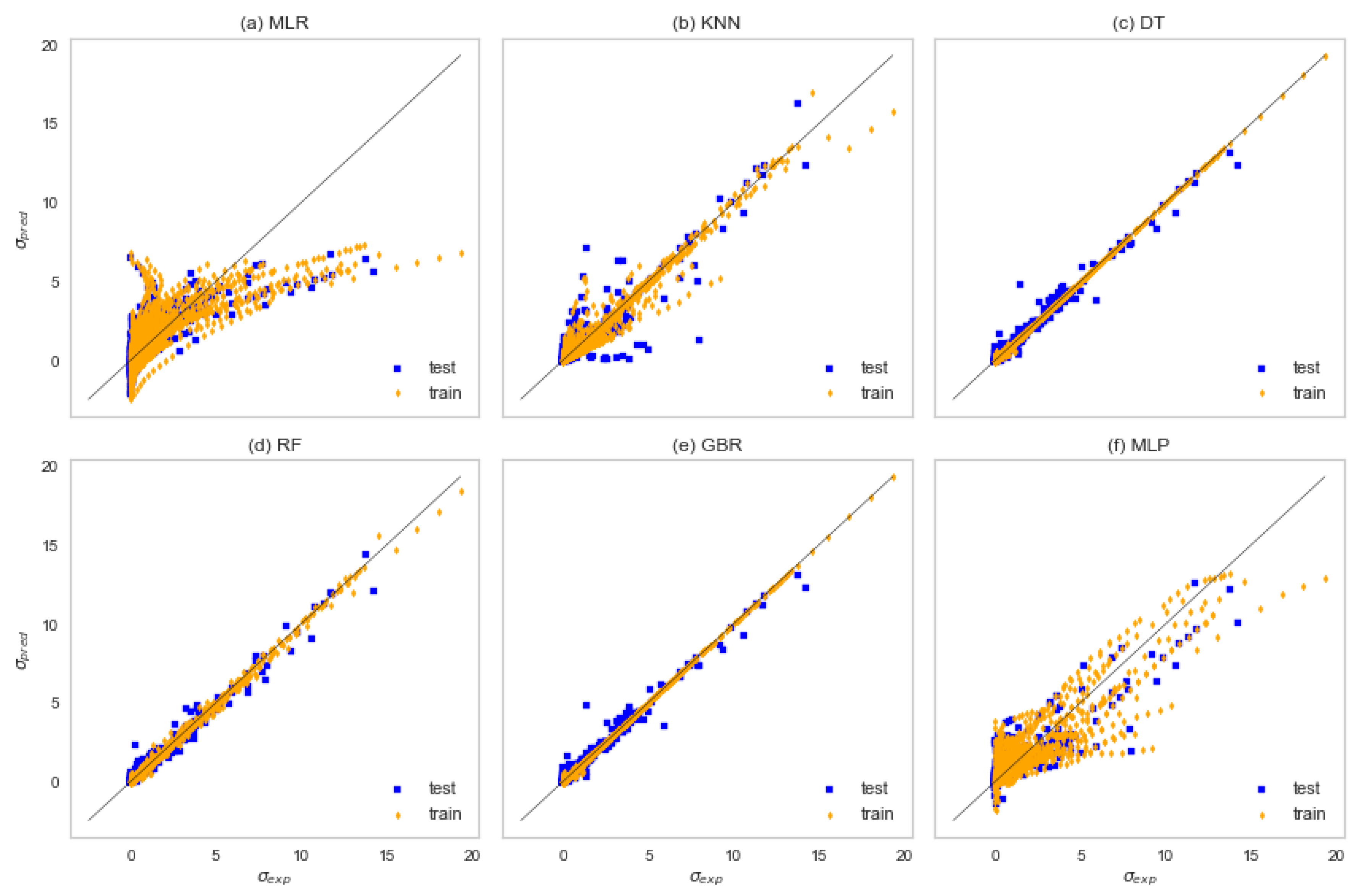
The results from the application of the numerical ML algorithms on the electrical conductivity dataset are gathered in Figure 6a–f, in identity plots that estimate the model’s accuracy by fitting the experimental and predicted data on the 45° diagonal line. The prediction is more accurate when the data points are set close to the line [78].
The linear regression method (MLR) in Figure 6a presented a rather poor fit for the ionic liquid data. This is somehow expected if we take into account the empirical relations from Equations (1)–(3), where the electrical conductivity value seems to have logarithmic dependence on the temperature or molecular volume. Thus, we expected that nonlinear ML methods would achieve better results. The KNN algorithm in Figure 6b showed better performance than MLR. Nevertheless, the three tree-based algorithms that follow in Figure 6c-e, i.e., DT, RF, and GBR, respectively, fit well on the experimental data, as it seems that their tree structure was better suited to the problem. The neural network (NN) architecture in Figure 6f did not achieve adequate prediction capability for the specific implementation (three hidden layers of 20 nodes each). We also tested different architectures with trial-and-error procedures but did not manage to obtain better results. However, NNs are a distinct field of investigation, and further investigation is needed to find the optimal architecture, which is beyond the scope of this paper. Conclusively, it was shown that most of the algorithms investigated here (except for MLR) achieved acceptable prediction performance on the available dataset.
The accuracy metrics for the fittings shown in Figure 6, such as R2, MSE, MAE, and AAD, are shown in Table 1. The table values confirmed our observations that the three-based algorithms achieved the best fit on the data, as the coefficient of the determination reached values close to unity (R2 = 0.99), while a minimum number of errors were expressed by MAE and MSE, compared with the remaining algorithms. However, the AAD values differed significantly. The AAD value expresses the average sum of the errors derived from the distance of the predicted data around the experimental base data. From Table 1, it is evident that the GBR method is superior to RF, followed by DT.
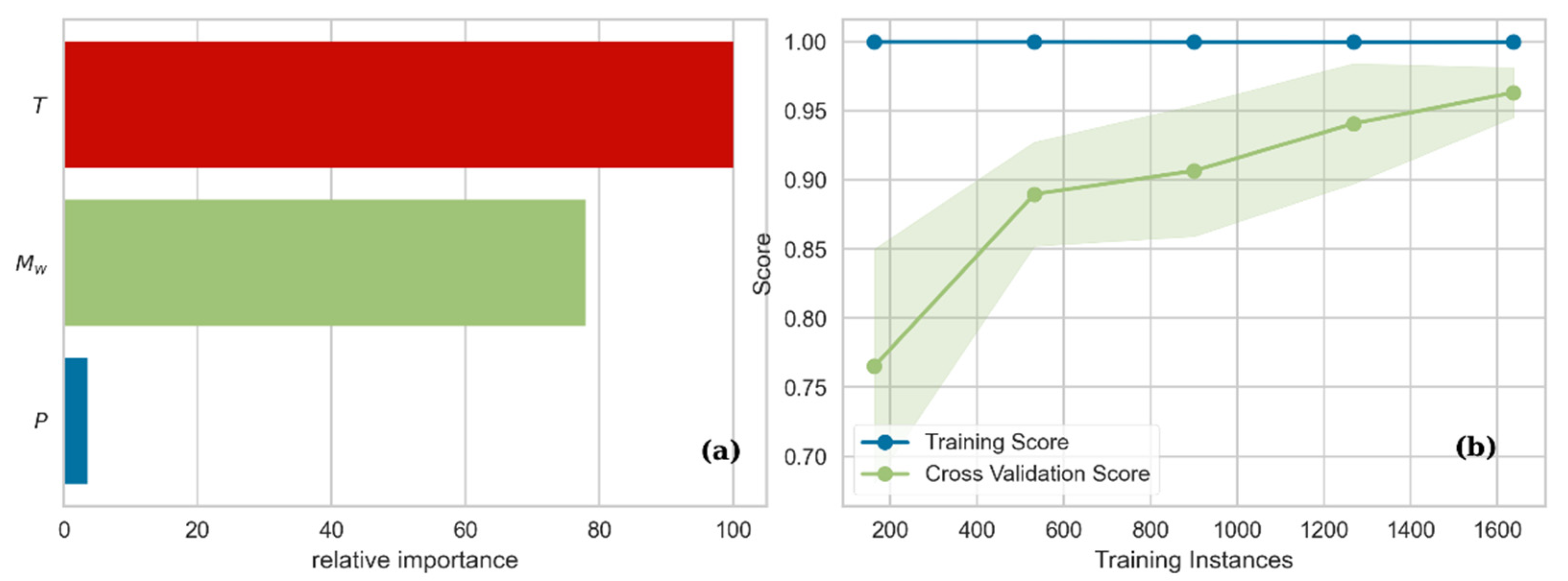
Let us now turn our attention to finding the most important input feature that controls the internal mechanism of the algorithmic decisions for the GBR. The feature importance plot in Figure 7a presents an estimation of the importance of each input variable on the prediction of the electrical conductivity value. Temperature, T, was found to be the most important parameter that guided the decisions between the DTs and the branches of the GBR architecture. This is in agreement with the widely used empirical Equations (1)–(2), where T is the only parameter that affects electrical conductivity. The next important feature was the molecular weight, Mw, as it was the main parameter in the proposed model that differentiated between the various types of incorporated ILs. Pressure, P, had only a small effect on the final result. As is also shown in the partial dependence plot of Figure 5, P affected σ only for small values (around P = 100 kPa), and no effect was observed above this limit.
Another important outcome to aid in the interpretation of the ML model is the learning curve diagram in Figure 7b, which reveals if the proposed algorithm was efficiently trained on the dataset. This is connected to the ability of the algorithm to make new predictions. Here, we observe that the cross-validation score increased as the number of training data points increased, reaching the highest value after about 1500 data points. This is evidence that the dataset used in this model (2274 data points) is capable of providing accurate predictions that could be generalized in research cases inside and outside the range of the parameters that constitute the dataset.
3.3. Obtaining an Analytical Expression
Symbolic regression is capable of providing analytical expressions to fit the dataset under investigation, without a priori knowledge of the system. This means that the SR algorithm starts with the random construction of expressions and iteratively searches for the best candidate equation. The proposed equations are of various complexity levels, and the choice of a simple or a more complicated one depends on the application and the desired accuracy. Here, we present three possible expressions that describe the electrical conductivity, σ, of ionic liquids, with input variables T, Mw, and P. Table 2 presents the mathematical expressions, along with calculated metrics.
The SR algorithm proposed three different classes of solutions, namely an exponential form (σ1), a nonlinear fractional form (σ2), and a combined fractional/square root form (σ3). These forms appeared at most in the output expression pool. We have to note here that the SR output included a total of 20 equations, with increasing complexity Comp. = 1–20, per iteration run, for 40 parallel runs (for more details refer to [76]), i.e., 800 candidate expressions.
We observe that Equation captured the exponential behavior shown in empirical Equation 1; however, one could not directly compare the two equations since Equation considered and P apart from T. Nonetheless, this is a simple equation that captures the ionic liquid physical behavior, with satisfying error metrics, but its disadvantage is the high AAD value, denoting increased distance from the real experimental values. The increased complexity of Equations and yielded better error metrics, with Equation reaching R2 = 0.883 and Equation having the smallest AAD = 149,183.5.
4. Conclusions
Ionic liquid research is a field of investigation mainly based on experimental measurements, and fundamental information is hard to obtain. The need for incorporating novel computational techniques has opened the road to ML techniques that can assist in this direction.
We incorporated various ML algorithms in this paper that showed a good fit on the employed ionic liquid dataset for the electrical conductivity prediction. The best fit was obtained for the GBR algorithm, for which its tree-based procedure and the ensemble approach to processing the data successfully captured the electrical conductivity behavior. Notwithstanding the fact that numerical ML algorithms performed well on their predictions, the SR-based investigation also presented in this paper approached the problem analytically, providing mathematical expressions that can be used without further implications, thus overcoming the black-box nature of numerical ML algorithms.
We believe that by further enriching the dataset with the values deriving from either experiments or carefully established molecular simulations, ML data-driven techniques can become part of the property calculations of ionic liquids. It is of importance to suggest novel evolutional processes, reliable pre- and post-processing techniques, and physics-oriented justification to establish an integrated computational platform that can be used by scientists and engineers who wish to harness the vast volume of data involved in their field.
Supplementary Materials
The following supporting information can be downloaded at: https://www.mdpi.com/10.3390/fluids7100321/s1, Table S1: The database of ILs incorporated for our model, with 2274 data points; Table S2: Ionic Liquids Database.
Author Contributions
Conceptualization, C.T.; funding acquisition, F.S.; methodology, F.S.; software, F.S.; supervision, T.E.K.; visualization, F.S.; writing—original draft preparation, F.S. and T.E.K.; writing—review and editing, T.E.K. and C.T. All authors have read and agreed to the published version of the manuscript.
Funding
F.S. acknowledges support from the project CAMINOS (No. 5600.03.08.03), which is implemented in the context of a grant by the Center of Research Innovation and Excellence of U. Th., funded by the Special Account for Research Grants of U. Th.
Institutional Review Board Statement
Not applicable.
Informed Consent Statement
Not applicable.
Data Availability Statement
All data are extracted from NIST Ionic Liquid Database (ILThermo) available online: https://ilthermo.boulder.nist.gov/ (accessed on 4 August 2022) and provided in Supplementary Material File S2.
Acknowledgments
We acknowledge computational time granted from the National Infrastructures for Research and Technology S.A. (GRNET S.A.) in the National HPC facility—ARIS.
Conflicts of Interest
The authors declare no conflict of interest.
References
- Ward, L.; Wolverton, C. Atomistic calculations and materials informatics: A review. Curr. Opin. Solid State Mater. Sci. 2017, 21, 167–176. [Google Scholar] [CrossRef]
- Frank, M.; Drikakis, D.; Charissis, V. Machine-Learning Methods for Computational Science and Engineering. Computation 2020, 8, 15. [Google Scholar] [CrossRef] [Green Version]
- Ramprasad, R.; Batra, R.; Pilania, G.; Mannodi-Kanakkithodi, A.; Kim, C. Machine learning in materials informatics: Recent applications and prospects. npj Comput. Mater. 2017, 3, 54. [Google Scholar] [CrossRef] [Green Version]
- Gao, C.; Min, X.; Fang, M.; Tao, T.; Zheng, X.; Liu, Y.; Wu, X.; Huang, Z. Innovative Materials Science via Machine Learning. Adv. Funct. Mater. 2022, 32, 2108044. [Google Scholar] [CrossRef]
- Craven, G.T.; Lubbers, N.; Barros, K.; Tretiak, S. Machine learning approaches for structural and thermodynamic properties of a Lennard-Jones fluid. J. Chem. Phys. 2020, 153, 104502. [Google Scholar] [CrossRef]
- Sun, W.; Zheng, Y.; Yang, K.; Zhang, Q.; Shah, A.A.; Wu, Z.; Sun, Y.; Feng, L.; Chen, D.; Xiao, Z.; et al. Machine learning-assisted molecular design and efficiency prediction for high-performance organic photovoltaic materials. Sci. Adv. 2019, 5, eaay4275. [Google Scholar] [CrossRef] [Green Version]
- Voyles, P.M. Informatics and data science in materials microscopy. Curr. Opin. Solid State Mater. Sci. 2017, 21, 141–158. [Google Scholar] [CrossRef]
- Davies, M.B.; Fitzner, M.; Michaelides, A. Accurate prediction of ice nucleation from room temperature water. Proc. Natl. Acad. Sci. USA 2022, 119, e2205347119. [Google Scholar] [CrossRef]
- Deringer, V.L.; Bartók, A.P.; Bernstein, N.; Wilkins, D.M.; Ceriotti, M.; Csányi, G. Gaussian Process Regression for Materials and Molecules. Chem. Rev. 2021, 121, 10073–10141. [Google Scholar] [CrossRef]
- Boussaidi, M.A.; Ren, O.; Voytsekhovsky, D.; Manzhos, S. Random Sampling High Dimensional Model Representation Gaussian Process Regression (RS-HDMR-GPR) for Multivariate Function Representation: Application to Molecular Potential Energy Surfaces. J. Phys. Chem. A 2020, 124, 7598–7607. [Google Scholar] [CrossRef]
- Alber, M.; Buganza Tepole, A.; Cannon, W.R.; De, S.; Dura-Bernal, S.; Garikipati, K.; Karniadakis, G.; Lytton, W.W.; Perdikaris, P.; Petzold, L.; et al. Integrating machine learning and multiscale modeling—Perspectives, challenges, and opportunities in the biological, biomedical, and behavioral sciences. npj Digit. Med. 2019, 2, 115. [Google Scholar] [CrossRef] [PubMed] [Green Version]
- Sofos, F.; Stavrogiannis, C.; Exarchou-Kouveli, K.K.; Akabua, D.; Charilas, G.; Karakasidis, T.E. Current Trends in Fluid Research in the Era of Artificial Intelligence: A Review. Fluids 2022, 7, 116. [Google Scholar] [CrossRef]
- Schran, C.; Thiemann, F.L.; Rowe, P.; Müller, E.A.; Marsalek, O.; Michaelides, A. Machine learning potentials for complex aqueous systems made simple. Proc. Natl. Acad. Sci. USA 2021, 118, e2110077118. [Google Scholar] [CrossRef]
- Karniadakis, G.E.; Kevrekidis, I.G.; Lu, L.; Perdikaris, P.; Wang, S.; Yang, L. Physics-informed machine learning. Nat. Rev. Phys. 2021, 3, 422–440. [Google Scholar] [CrossRef]
- Alam, T.M.; Allers, J.P.; Leverant, C.J.; Harvey, J.A. Symbolic regression development of empirical equations for diffusion in Lennard-Jones fluids. J. Chem. Phys. 2022, 157, 014503. [Google Scholar] [CrossRef] [PubMed]
- Papastamatiou, K.; Sofos, F.; Karakasidis, T.E. Machine learning symbolic equations for diffusion with physics-based descriptions. AIP Adv. 2022, 12, 025004. [Google Scholar] [CrossRef]
- Marsh, K.N.; Boxall, J.A.; Lichtenthaler, R. Room temperature ionic liquids and their mixtures—A review. Fluid Phase Equilibria 2004, 219, 93–98. [Google Scholar] [CrossRef]
- Gao, T.; Itliong, J.; Kumar, S.P.; Hjorth, Z.; Nakamura, I. Polarization of ionic liquid and polymer and its implications for polymerized ionic liquids: An overview towards a new theory and simulation. J. Polym. Sci. 2021, 59, 2434–2457. [Google Scholar] [CrossRef]
- Mousavi, S.P.; Atashrouz, S.; Nait Amar, M.; Hemmati-Sarapardeh, A.; Mohaddespour, A.; Mosavi, A. Viscosity of Ionic Liquids: Application of the Eyring’s Theory and a Committee Machine Intelligent System. Molecules 2021, 26, 156. [Google Scholar] [CrossRef]
- Earle, M.J.; Esperança, J.M.S.S.; Gilea, M.A.; Canongia Lopes, J.N.; Rebelo, L.P.N.; Magee, J.W.; Seddon, K.R.; Widegren, J.A. The distillation and volatility of ionic liquids. Nature 2006, 439, 831–834. [Google Scholar] [CrossRef]
- Armand, M.; Endres, F.; MacFarlane, D.R.; Ohno, H.; Scrosati, B. Ionic-liquid materials for the electrochemical challenges of the future. Nat. Mater. 2009, 8, 621–629. [Google Scholar] [CrossRef] [PubMed]
- Koutsoumpos, S.; Giannios, P.; Stavrakas, I.; Moutzouris, K. The derivative method of critical-angle refractometry for attenuating media. J. Opt. 2020, 22, 075601. [Google Scholar] [CrossRef]
- Tsuda, T.; Kawakami, K.; Mochizuki, E.; Kuwabata, S. Ionic liquid-based transmission electron microscopy for herpes simplex virus type 1. Biophys. Rev. 2018, 10, 927–929. [Google Scholar] [CrossRef] [PubMed]
- Xu, L.; Cui, X.; Zhang, Y.; Feng, T.; Lin, R.; Li, X.; Jie, H. Measurement and correlation of electrical conductivity of ionic liquid [EMIM][DCA] in propylene carbonate and γ-butyrolactone. Electrochim. Acta 2015, 174, 900–907. [Google Scholar] [CrossRef]
- Koutsoukos, S.; Philippi, F.; Malaret, F.; Welton, T. A review on machine learning algorithms for the ionic liquid chemical space. Chem. Sci. 2021, 12, 6820–6843. [Google Scholar] [CrossRef]
- Duong, D.V.; Tran, H.-V.; Pathirannahalage, S.K.; Brown, S.J.; Hassett, M.; Yalcin, D.; Meftahi, N.; Christofferson, A.J.; Greaves, T.L.; Le, T.C. Machine learning investigation of viscosity and ionic conductivity of protic ionic liquids in water mixtures. J. Chem. Phys. 2022, 156, 154503. [Google Scholar] [CrossRef] [PubMed]
- Daryayehsalameh, B.; Nabavi, M.; Vaferi, B. Modeling of CO2 capture ability of [Bmim][BF4] ionic liquid using connectionist smart paradigms. Environ. Technol. Innov. 2021, 22, 101484. [Google Scholar] [CrossRef]
- Beckner, W.; Ashraf, C.; Lee, J.; Beck, D.A.C.; Pfaendtner, J. Continuous Molecular Representations of Ionic Liquids. J. Phys. Chem. B 2020, 124, 8347–8357. [Google Scholar] [CrossRef]
- Bulut, S.; Eiden, P.; Beichel, W.; Slattery, J.M.; Beyersdorff, T.F.; Schubert, T.J.S.; Krossing, I. Temperature Dependence of the Viscosity and Conductivity of Mildly Functionalized and Non-Functionalized [Tf2N]−Ionic Liquids. ChemPhysChem 2011, 12, 2296–2310. [Google Scholar] [CrossRef]
- Leys, J.; Wübbenhorst, M.; Preethy Menon, C.; Rajesh, R.; Thoen, J.; Glorieux, C.; Nockemann, P.; Thijs, B.; Binnemans, K.; Longuemart, S. Temperature dependence of the electrical conductivity of imidazolium ionic liquids. J. Chem. Phys. 2008, 128, 064509. [Google Scholar] [CrossRef]
- Rodil, E.; Arce, A.; Arce, A.; Soto, A. Measurements of the density, refractive index, electrical conductivity, thermal conductivity and dynamic viscosity for tributylmethylphosphonium and methylsulfate based ionic liquids. Thermochim. Acta 2018, 664, 81–90. [Google Scholar] [CrossRef]
- Bandrés, I.; Montaño, D.F.; Gascón, I.; Cea, P.; Lafuente, C. Study of the conductivity behavior of pyridinium-based ionic liquids. Electrochim. Acta 2010, 55, 2252–2257. [Google Scholar] [CrossRef]
- Slattery, J.M.; Daguenet, C.; Dyson, P.J.; Schubert, T.J.S.; Krossing, I. How to Predict the Physical Properties of Ionic Liquids: A Volume-Based Approach. Angew. Chem. Int. Ed. 2007, 46, 5384–5388. [Google Scholar] [CrossRef] [PubMed]
- Beichel, W.; Preiss, U.P.; Verevkin, S.P.; Koslowski, T.; Krossing, I. Empirical description and prediction of ionic liquids’ properties with augmented volume-based thermodynamics. J. Mol. Liq. 2014, 192, 3–8. [Google Scholar] [CrossRef]
- Ionic Liquids Database-ILThermo. NIST Standard Reference Database #147. Available online: https://ilthermo.boulder.nist.gov/ (accessed on 4 August 2022).
- Dong, Q.; Muzny, C.D.; Kazakov, A.; Diky, V.; Magee, J.W.; Widegren, J.A.; Chirico, R.D.; Marsh, K.N.; Frenkel, M. ILThermo: A Free-Access Web Database for Thermodynamic Properties of Ionic Liquids. J. Chem. Eng. Data 2007, 52, 1151–1159. [Google Scholar] [CrossRef]
- Zec, N.; Bešter-Rogač, M.; Vraneš, M.; Gadžurić, S. Physicochemical properties of (1-butyl-1-methylpyrrolydinium dicyanamide+γ-butyrolactone) binary mixtures. J. Chem. Thermodyn. 2015, 91, 327–335. [Google Scholar] [CrossRef]
- Vila, J.; Fernández-Castro, B.; Rilo, E.; Carrete, J.; Domínguez-Pérez, M.; Rodríguez, J.R.; García, M.; Varela, L.M.; Cabeza, O. Liquid–solid–liquid phase transition hysteresis loops in the ionic conductivity of ten imidazolium-based ionic liquids. Fluid Phase Equilibria 2012, 320, 1–10. [Google Scholar] [CrossRef]
- Harris, K.R.; Kanakubo, M.; Kodama, D.; Makino, T.; Mizuguchi, Y.; Watanabe, M.; Watanabe, T. Temperature and Density Dependence of the Transport Properties of the Ionic Liquid Triethylpentylphosphonium Bis(trifluoromethanesulfonyl)amide, [P222,5][Tf2N]. J. Chem. Eng. Data 2018, 63, 2015–2027. [Google Scholar] [CrossRef]
- Harris, K.R.; Kanakubo, M.; Tsuchihashi, N.; Ibuki, K.; Ueno, M. Effect of Pressure on the Transport Properties of Ionic Liquids: 1-Alkyl-3-methylimidazolium Salts. J. Phys. Chem. B 2008, 112, 9830–9840. [Google Scholar] [CrossRef]
- Vranes, M.; Dozic, S.; Djeric, V.; Gadzuric, S. Physicochemical Characterization of 1-Butyl-3-methylimidazolium and 1-Butyl-1-methylpyrrolidinium Bis(trifluoromethylsulfonyl)imide. J. Chem. Eng. Data 2012, 57, 1072–1077. [Google Scholar] [CrossRef]
- Kanakubo, M.; Harris, K.R.; Tsuchihashi, N.; Ibuki, K.; Ueno, M. Temperature and pressure dependence of the electrical conductivity of the ionic liquids 1-methyl-3-octylimidazolium hexafluorophosphate and 1-methyl-3-octylimidazolium tetrafluoroborate. Fluid Phase Equilibria 2007, 261, 414–420. [Google Scholar] [CrossRef]
- Kanakubo, M.; Harris, K.R.; Tsuchihashi, N.; Ibuki, K.; Ueno, M. Effect of Pressure on Transport Properties of the Ionic Liquid 1-Butyl-3-methylimidazolium Hexafluorophosphate. J. Phys. Chem. B 2007, 111, 2062–2069. [Google Scholar] [CrossRef] [PubMed]
- Oleinikova, A.; Bonetti, M. Critical Behavior of the Electrical Conductivity of Concentrated Electrolytes: Ethylammonium Nitrate in n-Octanol Binary Mixture. J. Solut. Chem. 2002, 31, 397–413. [Google Scholar] [CrossRef]
- Kanakubo, M.; Harris, K.R. Density of 1-Butyl-3-methylimidazolium Bis(trifluoromethanesulfonyl)amide and 1-Hexyl-3-methylimidazolium Bis(trifluoromethanesulfonyl)amide over an Extended Pressure Range up to 250 MPa. J. Chem. Eng. Data 2015, 60, 1408–1418. [Google Scholar] [CrossRef]
- Vila, J.; Ginés, P.; Pico, J.M.; Franjo, C.; Jiménez, E.; Varela, L.M.; Cabeza, O. Temperature dependence of the electrical conductivity in EMIM-based ionic liquids: Evidence of Vogel–Tamman–Fulcher behavior. Fluid Phase Equilibria 2006, 242, 141–146. [Google Scholar] [CrossRef]
- Machanová, K.; Boisset, A.; Sedláková, Z.; Anouti, M.; Bendová, M.; Jacquemin, J. Thermophysical Properties of Ammonium-Based Bis{(trifluoromethyl)sulfonyl}imide Ionic Liquids: Volumetric and Transport Properties. Chem. Eng. Data 2012, 57, 2227–2235. [Google Scholar] [CrossRef] [Green Version]
- Rad-Moghadam, K.; Hassani, S.A.R.M.; Roudsari, S.T. N-methyl-2-pyrrolidonium chlorosulfonate: An efficient ionic-liquid catalyst and mild sulfonating agent for one-pot synthesis of δ-sultones. J. Mol. Liq. 2016, 218, 275–280. [Google Scholar] [CrossRef]
- Fleshman, A.M.; Mauro, N.A. Temperature-dependent structure and transport of ionic liquids with short-and intermediate-chain length pyrrolidinium cations. J. Mol. Liq. 2019, 279, 23–31. [Google Scholar] [CrossRef]
- Nazet, A.; Sokolov, S.; Sonnleitner, T.; Makino, T.; Kanakubo, M.; Buchner, R. Densities, Viscosities, and Conductivities of the Imidazolium Ionic Liquids [Emim][Ac], [Emim][FAP], [Bmim][BETI], [Bmim][FSI], [Hmim][TFSI], and [Omim][TFSI]. J. Chem. Eng. Data 2015, 60, 2400–2411. [Google Scholar] [CrossRef]
- Abdurrokhman, I.; Elamin, K.; Danyliv, O.; Hasani, M.; Swenson, J.; Martinelli, A. Protic Ionic Liquids Based on the Alkyl-Imidazolium Cation: Effect of the Alkyl Chain Length on Structure and Dynamics. J. Phys. Chem. B 2019, 123, 4044–4054. [Google Scholar] [CrossRef]
- Bandrés, I.; Carmen López, M.; Castro, M.; Barberá, J.; Lafuente, C. Thermophysical properties of 1-propylpyridinium tetrafluoroborate. J. Chem. Thermodyn. 2012, 44, 148–153. [Google Scholar] [CrossRef] [Green Version]
- García-Mardones, M.; Bandrés, I.; López, M.C.; Gascón, I.; Lafuente, C. Experimental and Theoretical Study of Two Pyridinium-Based Ionic Liquids. J Solut. Chem. 2012, 41, 1836–1852. [Google Scholar] [CrossRef]
- Yamamoto, T.; Matsumoto, K.; Hagiwara, R.; Nohira, T. Physicochemical and Electrochemical Properties of K[N(SO2F)2]–[N-Methyl-N-propylpyrrolidinium][N(SO2F)2] Ionic Liquids for Potassium-Ion Batteries. J. Phys. Chem. C 2017, 121, 18450–18458. [Google Scholar] [CrossRef]
- Cabeza, O.; Vila, J.; Rilo, E.; Domínguez-Pérez, M.; Otero-Cernadas, L.; López-Lago, E.; Méndez-Morales, T.; Varela, L.M. Physical properties of aqueous mixtures of the ionic 1-ethl-3-methyl imidazolium octyl sulfate: A new ionic rigid gel. J. Chem. Thermodyn. 2014, 75, 52–57. [Google Scholar] [CrossRef]
- Stoppa, A.; Zech, O.; Kunz, W.; Buchner, R. The Conductivity of Imidazolium-Based Ionic Liquids from (−35 to 195) °C. A. Variation of Cation’s Alkyl Chain. J. Chem. Eng. Data 2010, 55, 1768–1773. [Google Scholar] [CrossRef]
- Zech, O.; Stoppa, A.; Buchner, R.; Kunz, W. The Conductivity of Imidazolium-Based Ionic Liquids from (248 to 468) K. B. Variation of the Anion. J. Chem. Eng. Data 2010, 55, 1774–1778. [Google Scholar] [CrossRef]
- Nazet, A.; Sokolov, S.; Sonnleitner, T.; Friesen, S.; Buchner, R. Densities, Refractive Indices, Viscosities, and Conductivities of Non-Imidazolium Ionic Liquids [Et3S][TFSI], [Et2MeS][TFSI], [BuPy][TFSI], [N8881][TFA], and [P14][DCA]. J. Chem. Eng. Data 2017, 62, 2549–2561. [Google Scholar] [CrossRef]
- Benito, J.; García-Mardones, M.; Pérez-Gregorio, V.; Gascón, I.; Lafuente, C. Physicochemical Study of n-Ethylpyridinium bis(trifluoromethylsulfonyl)imide Ionic Liquid. J Solut. Chem. 2014, 43, 696–710. [Google Scholar] [CrossRef]
- Kasprzak, D.; Stępniak, I.; Galiński, M. Electrodes and hydrogel electrolytes based on cellulose: Fabrication and characterization as EDLC components. J. Solid State Electrochem. 2018, 22, 3035–3047. [Google Scholar] [CrossRef] [Green Version]
- Brunton, S.L.; Noack, B.R.; Koumoutsakos, P. Machine Learning for Fluid Mechanics. Annu. Rev. Fluid Mech. 2020, 52, 477–508. [Google Scholar] [CrossRef]
- Pedregosa, F.; Varoquaux, G.; Gramfort, A.; Michel, V.; Thirion, B.; Grisel, O.; Blondel, M.; Prettenhofer, P.; Weiss, R.; Dubourg, V.; et al. Scikit-learn: Machine Learning in Python. J. Mach. Learn. Res. 2011, 12, 2825–2830. [Google Scholar]
- Cranmer, M.; Sanchez Gonzalez, A.; Battaglia, P.; Xu, R.; Cranmer, K.; Spergel, D.; Ho, S. Discovering symbolic models from deep learning with inductive biases. In Proceedings of the 34th Conference on Neural Information Processing Systems (NeurIPS 2020), Vancouver, BC, Canada, 6–12 December 2020; Larochelle, H., Ranzato, M., Hadsell, R., Balcan, M.F., Lin, H., Eds.; Curran Associates, Inc.: New York, NY, USA, 2020; Volume 33, pp. 17429–17442. [Google Scholar]
- Uyanık, G.K.; Güler, N. A Study on Multiple Linear Regression Analysis. Procedia-Soc. Behav. Sci. 2013, 106, 234–240. [Google Scholar] [CrossRef] [Green Version]
- Rahman, J.; Ahmed, K.S.; Khan, N.I.; Islam, K.; Mangalathu, S. Data-driven shear strength prediction of steel fiber reinforced concrete beams using machine learning approach. Eng. Struct. 2021, 233, 111743. [Google Scholar] [CrossRef]
- Song, Y.; Liang, J.; Lu, J.; Zhao, X. An efficient instance selection algorithm for k nearest neighbor regression. Neurocomputing 2017, 251, 26–34. [Google Scholar] [CrossRef]
- Loh, W.-Y. Classification and regression trees. WIREs Data Min. Knowl. Discov. 2011, 1, 14–23. [Google Scholar] [CrossRef]
- Schmidt, J.; Marques, M.R.G.; Botti, S.; Marques, M.A.L. Recent advances and applications of machine learning in solid-state materials science. npj Comput. Mater. 2019, 5, 83. [Google Scholar] [CrossRef] [Green Version]
- Sofos, F.; Karakasidis, T.E. Nanoscale slip length prediction with machine learning tools. Sci. Rep. 2021, 11, 12520. [Google Scholar] [CrossRef]
- Allers, J.P.; Harvey, J.A.; Garzon, F.H.; Alam, T.M. Machine learning prediction of self-diffusion in Lennard-Jones fluids. J. Chem. Phys. 2020, 153, 034102. [Google Scholar] [CrossRef]
- Sandhu, A.K.; Batth, R.S. Software reuse analytics using integrated random forest and gradient boosting machine learning algorithm. Softw Pract. Exp. 2021, 51, 735–747. [Google Scholar] [CrossRef]
- Jerome, H. Friedman Greedy function approximation: A gradient boosting machine. Ann. Stat. 2001, 29, 1189–1232. [Google Scholar] [CrossRef]
- Stathakis, D. How Many Hidden Layers and Nodes? Int. J. Remote Sens. 2009, 30, 2133–2147. [Google Scholar] [CrossRef]
- Kingma, D.P.; Ba, J. Adam: A Method for Stochastic Optimization. arXiv 2015, 6908. [Google Scholar] [CrossRef]
- Wang, Y.; Wagner, N.; Rondinelli, J.M. Symbolic regression in materials science. MRS Commun. 2019, 9, 793–805. [Google Scholar] [CrossRef] [Green Version]
- Sofos, F.; Charakopoulos, A.; Papastamatiou, K.; Karakasidis, T.E. A combined clustering/symbolic regression framework for fluid property prediction. Phys. Fluids 2022, 34, 062004. [Google Scholar] [CrossRef]
- Agrawal, A.; Deshpande, P.D.; Cecen, A.; Basavarsu, G.P.; Choudhary, A.N.; Kalidindi, S.R. Exploration of data science techniques to predict fatigue strength of steel from composition and processing parameters. Integr. Mater. Manuf. Innov. 2014, 3, 90–108. [Google Scholar] [CrossRef] [Green Version]
- Bengfort, B.; Bilbro, R. Yellowbrick: Visualizing the Scikit-Learn Model Selection Process. J. Open Source Softw. 2019, 4, 1075. [Google Scholar] [CrossRef]
Figure 1.
Machine learning model for electrical conductivity prediction, providing both numerical and analytical output.
Figure 1.
Machine learning model for electrical conductivity prediction, providing both numerical and analytical output.

Figure 2.
Correlation matrix for the three inputs and the output, σ.

Figure 3.
A pair plot diagram, showing input and output parameter distribution. The diagonal bar plots display the distribution of each parameter, while the remaining figures are scatter plots between all input pairs.
Figure 3.
A pair plot diagram, showing input and output parameter distribution. The diagonal bar plots display the distribution of each parameter, while the remaining figures are scatter plots between all input pairs.

Figure 4.
Graphical implementation of ML algorithms incorporated in this paper: (a) multiple linear regression; (b) k-nearest neighbors; (c) decision tree, (d) random forest; (e) gradient boosting regressor; (f) multi-layer perceptron; (g) symbolic regression.
Figure 4.
Graphical implementation of ML algorithms incorporated in this paper: (a) multiple linear regression; (b) k-nearest neighbors; (c) decision tree, (d) random forest; (e) gradient boosting regressor; (f) multi-layer perceptron; (g) symbolic regression.

Figure 5.
Partial dependence plot, where each input is investigated on the effect on electrical conductivity (σ). (a) molecular weight; (b) temperature; (c) pressure.
Figure 5.
Partial dependence plot, where each input is investigated on the effect on electrical conductivity (σ). (a) molecular weight; (b) temperature; (c) pressure.

Figure 6.
Experimental vs. predicted values for electrical conductivity with six different ML algorithms: (a) MLR; (b) KNN; (c) DT; (d) RI (e) GBR; (f) MLP. The 45o straight line denotes perfect match.
Figure 6.
Experimental vs. predicted values for electrical conductivity with six different ML algorithms: (a) MLR; (b) KNN; (c) DT; (d) RI (e) GBR; (f) MLP. The 45o straight line denotes perfect match.

Figure 7.
Interpretation output diagrams from the application of GBR algorithm on the prediction of electrical conductivity: (a) feature importance plot; (b) learning curve diagram.
Figure 7.
Interpretation output diagrams from the application of GBR algorithm on the prediction of electrical conductivity: (a) feature importance plot; (b) learning curve diagram.


Table 1.
Accuracy metrics and comparison of 6 ML algorithms for the ionic liquids’ dataset.
| Algorithm | R2 | MAE | MSE | AAD |
|---|---|---|---|---|
| MLR | 0.69701 | 1.02 | 2.287 | 663720.1 |
| KNN | 0.91344 | 0.381 | 0.755 | 1265.019 |
| DT | 0.98916 | 0.138 | 0.098 | 536.7186 |
| RF | 0.98919 | 0.16 | 0.097 | 1635.613 |
| GBR | 0.98886 | 0.137 | 0.1 | 271.6886 |
| MLP | 0.86707 | 0.706 | 1.107 | 35444.57 |
Table 2.
The three SR-extracted equations for electrical conductivity and their respective accuracy metrics. Comp. is the equation complexity.
Table 2.
The three SR-extracted equations for electrical conductivity and their respective accuracy metrics. Comp. is the equation complexity.
| Equation | Comp. | R2 | MAE | MSE | AAD |
|---|---|---|---|---|---|
| 6 | 0.760 | 1.234 | 2.846 | 2,660,488.8 | |
| 19 | 0.857 | 0.727 | 1.392 | 149,183.5 | |
| 20 | 0.883 | 0.728 | 1.160 | 3,551,375.7 |
Publisher’s Note: MDPI stays neutral with regard to jurisdictional claims in published maps and institutional affiliations. |
© 2022 by the authors. Licensee MDPI, Basel, Switzerland. This article is an open access article distributed under the terms and conditions of the Creative Commons Attribution (CC BY) license (https://creativecommons.org/licenses/by/4.0/).
Share and Cite
MDPI and ACS Style
Karakasidis, T.E.; Sofos, F.; Tsonos, C. The Electrical Conductivity of Ionic Liquids: Numerical and Analytical Machine Learning Approaches. Fluids 2022, 7, 321. https://doi.org/10.3390/fluids7100321
AMA Style
Karakasidis TE, Sofos F, Tsonos C. The Electrical Conductivity of Ionic Liquids: Numerical and Analytical Machine Learning Approaches. Fluids. 2022; 7(10):321. https://doi.org/10.3390/fluids7100321
Chicago/Turabian StyleKarakasidis, Theodoros E., Filippos Sofos, and Christos Tsonos. 2022. "The Electrical Conductivity of Ionic Liquids: Numerical and Analytical Machine Learning Approaches" Fluids 7, no. 10: 321. https://doi.org/10.3390/fluids7100321