
Prediction and Optimization of Pile Bearing Capacity Considering Effects of Time


1
Department of Civil Engineering, Isfahan University of Technology, Isfahan 8415683111, Iran
2
School of Civil and Environmental Engineering, University of Technology Sydney, Ultimo, NSW 2007, Australia
3
Peter the Great St. Petersburg Polytechnic University, 195251 St. Petersburg, Russia
*
Author to whom correspondence should be addressed.
Mathematics 2022, 10(19), 3563; https://doi.org/10.3390/math10193563
Submission received: 16 July 2022
/
Revised: 10 September 2022
/
Accepted: 13 September 2022
/
Published: 29 September 2022
(This article belongs to the Special Issue Modeling and Simulation in Engineering, 2nd Edition)
Abstract
:Prediction of pile bearing capacity has been considered an unsolved problem for years. This study presents a practical solution for the preparation and maximization of pile bearing capacity, considering the effects of time after the end of pile driving. The prediction phase proposes an intelligent equation using a genetic programming (GP) model. Thus, pile geometry, soil properties, initial pile capacity, and time after the end of driving were considered predictors to predict pile bearing capacity. The developed GP equation provided an acceptable level of accuracy in estimating pile bearing capacity. In the optimization phase, the developed GP equation was used as input in two powerful optimization algorithms, namely, the artificial bee colony (ABC) and the grey wolf optimization (GWO), in order to obtain the highest bearing capacity of the pile, which corresponds to the optimum values for input parameters. Among these two algorithms, GWO obtained a higher value for pile capacity compared to the ABC algorithm. The introduced models and their modeling procedure in this study can be used to predict the ultimate capacity of piles in such projects.
Keywords:
pile bearing capacity; genetic programming; artificial bee colony; gray wolf optimization; optimization purposesMSC:
68Txx1. Introduction
Pile foundations are structural elements that are mainly used when the surface soil is weak and there is an urgent need to transfer the structural load to the further layers of the soil, or when soil settlement is an essential concern in the designing process. In terms of the pile’s role in load transmission, calculating the precise ultimate bearing capacity of pile foundations is an important topic for geotechnical engineers. Besides this, some scholars have indicated that pile bearing capacity can be considered as a time-dependent parameter, exhibiting an increasing trend after a specific period [1,2,3]. Pile setup is a geotechnical phenomenon referring to a time-dependent increase in the ultimate bearing capacity of pile foundations. It is assumed that pile setup occurs due to the dissipation of the excess pore water pressure (EPWP) generated as a result of pile installation [4].
Furthermore, it is widely accepted that this phenomenon develops by incorporating three main stages, including the non-uniform dissipation of EPWP, the uniform dissipation of EPWP, and aging [5]. Results of different studies indicate that setup considerably affects the side resistance, while when it comes to the tip resistance, it has exhibited less change or a decrease owing to relaxation [1,6,7,8,9,10]. Predicting the time-dependent bearing capacity of pile foundations has always been an interesting topic for researchers. Moreover, considering the pile setup, the design process of piles can be more economical.
Many studies have been presented in which analytical or numerical models were developed to forecast the pile setup [11,12,13]. One of the most well-known investigations in this area is a study conducted by Skov and Denver [14] to find an equation to estimate the pile setup. The setup equation was revised using different geotechnical properties to achieve this goal. Finally, a semi-empirical equation was proposed by them introducing a practical variable called setup parameter (A). This pioneering study was a starting point for other researchers. For example, Haque and Abu-Farsakh [6] published a paper in which the application of a nonlinear multivariable regression model in the prediction of pile setup was investigated. Although the studies conducted using this group of techniques were able to create an effective equation, pile setup is a complex issue considering the complicated soil–pile interaction. Therefore, analytical methods and regression analysis do not seem to be powerful enough for prediction purposes [15].
In recent years, several studies have presented the successful usage of intelligent algorithms to simulate complex problems in civil and geotechnical engineering [16,17,18,19,20,21,22,23,24,25,26,27,28,29]. Several scholars have highlighted the applicability of these techniques in predicting pile-related issues, e.g., pile capacity, settlement, lateral deflection [30,31,32,33]. In a study conducted by Lee and Lee [34], the application of artificial neural networks (ANNs) in the prediction of pile bearing capacity was investigated. The results of the model and in situ pile load tests were utilized to verify the developed model. Finally, it was concluded that the error back-propagation neural network used in this study had good performance since the maximum error in the prediction process did not exceed 25%. Shahin [35] utilized intelligent computing to model the axial capacity of pile foundations. For this purpose, an ANN technique was employed to predict the axial capacity of driven piles and drilled shafts using a total of 174 data points. Furthermore, a comparison was made between CPT-based methods and the ANN to evaluate their performances in the prediction area. The results indicated that ANN with a correlation coefficient of 0.85 and 0.97 for driven and drilled shaft validation datasets showed acceptable performance. Samui [36] investigated the application of the support vector machine as a powerful machine learning technique to estimate the pile bearing capacity. Three inputs, including penetration depth ratio, mean normal stress, and the number of bowls, were considered for this aim. Eventually, using evaluation criteria such as coefficient of correlation, the developed model predicted the pile bearing capacity with sufficient accuracy. In another study, Momeni et al. [37] used the results from 50 dynamic load tests to predict the bearing capacity of piles using an ANN-based predictive model optimized with a genetic algorithm. The final data indicated that the developed model, with a correlation coefficient of 0.99, successfully predicted the target very close to its actual value.
Other studies tried to improve the performance of the base intelligent models using optimization algorithms. For instance, Dehghanbanadaki et al. [38] used the gray wolf optimization (GWO) algorithm to enhance the performance of the adaptive neuro-fuzzy inference system (ANFIS) for estimating the ultimate bearing capacity of single driven piles. The results showed that the actual values of pile bearing capacity had been successfully estimated using the GWO-ANFIS model, and their results improved upon the ANFIS model. In another study implemented by Armaghani et al. [33], a combination of ANFIS and group data handling methods optimized with a competitive imperialism algorithm (ICA) was utilized to forecast the pile bearing capacity. Based on the data and the evaluation criteria, the proposed model could be considered a powerful technique regarding pile foundations’ design process.
Previous works did not include a time component in their input parameters, and their input parameters were mostly pile geometry-related. However, this study includes a separate input directly related to time, which is the main difference between this study and those published previously. Another contribution in this study is related to the optimization phase. An intelligent equation has been developed to predict pile capacity using the genetic programming (GP) technique. Then, the proposed GP equation is used in two optimization techniques, namely artificial bee colony (ABC) and GWO to maximize pile capacity. A database containing information about 256 data samples has been considered to achieve these goals. The models mentioned above and their results are discussed and compared to introduce a new procedure for predicting pile capacity.
The rest of this paper is organized as follows:
Section 2 describes the methodology background of the used models in predicting and optimizing pile capacity. Section 3 gives the needed information regarding the database used for modeling. Section 4 discusses the process of prediction models to develop a GP model and its evaluation. The optimization process regarding two algorithms, i.e., ABC and GWO, is given in Section 5. Section 6 discusses both the prediction and optimization phases. Section 7 and Section 8 describe limitations, future works, and concluding remarks of this study.
2. Methodology Background
2.1. Genetic Programming
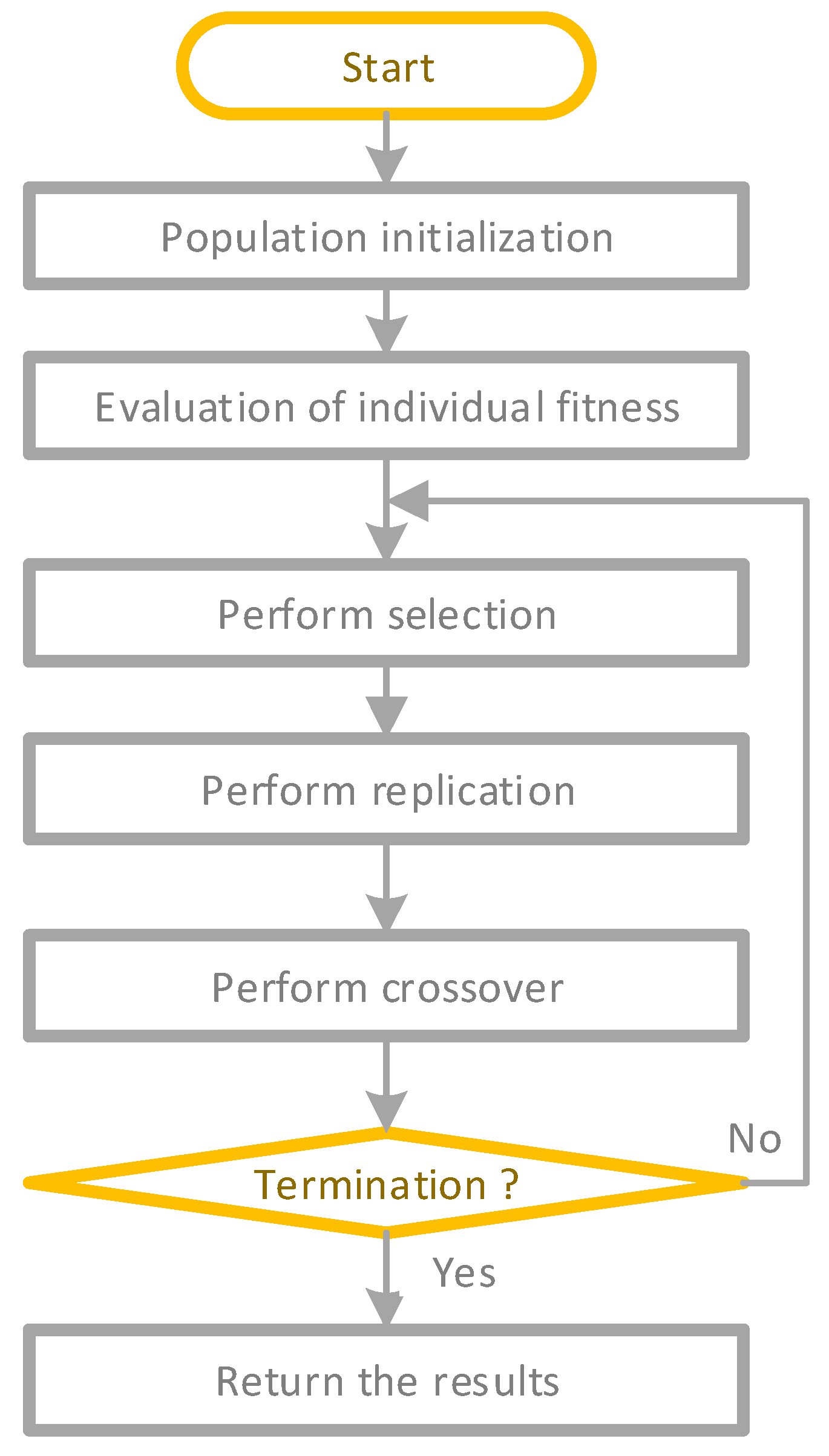
Genetic programming (GP) is an evolutionary computing algorithm [39], which simulates natural selection and biological evolution and automatically generates the best computer program based on the problem in the search space [40]. In GP, the individual represents the candidate’s solution to the problem. In the process of evolution, GP evaluates individual fitness, simulates the survival principle of survival of the fittest, and guides the population to carry out genetic operations (replication, crossover, and mutation) to renew the population. The goal of the GP algorithm is to gradually make some individuals in the population have better performance through several generations of evolution.
Figure 1 shows the flow chart to develop GP. First, a predetermined number of individuals are created as an initial population by randomly combining different elements of the function set and terminator set according to the program structure. Fitness values are then given to every individual. The fitness value reflects the ability of the individual to solve problems where the higher the value, the better the individual’s performance. After that, individuals are selected based on fitness values, and those with higher fitness are more likely to be selected. Genetic evolution of selected individuals is used to generate the next generation’s population. Individuals in the new population are repeatedly evaluated, selected, replicated, crossed, and mutated to complete genetic evolution. This stops when the maximum number of evolutions is reached or a certain condition is met. The best solution to the problem is the individual with the best fitness value.
2.2. Gray Wolf Optimization
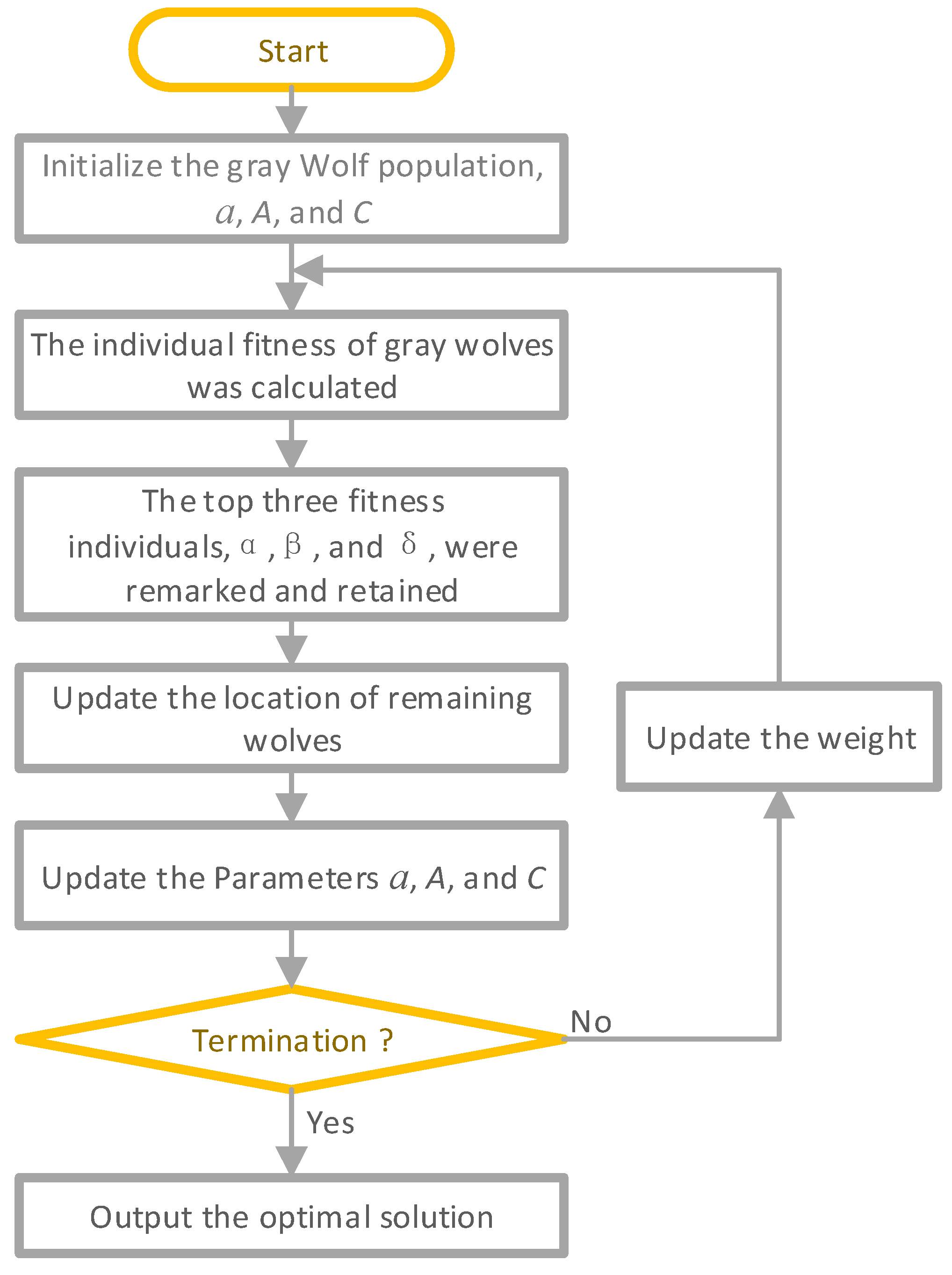
Gray wolf optimization (GWO) is a swarm-based optimization algorithm inspired by the predation behavior of wolves [41]. Compared with other traditional intelligent swarm algorithms, GWO has the advantages of fewer parameters, easy implementation, great convergence speed, and global search ability, so it has been widely used in many fields [42]. Through observation, it is found that wolves hunt mainly in three parts: first tracking, chasing, and approaching prey; then surrounding and harassing prey from all directions until it stops moving; and finally, attacking the prey. Figure 2 shows the process of GWO, a is based on a linear decrease iteration convergence factor, and A is the value in the interval [−2a, 2a], by setting the |a| < 1 or > 1 to implement the prey. C can be arbitrarily set in the interval [0,2], indicating the weight of prey affected by the position of the gray wolf. α, β and δ represent the potential superior solution of the optimization objective, where α is the optimal solution, β is the suboptimal solution, and δ is the third optimal solution.
2.3. Artificial Bee Colony
An artificial bee colony (ABC) is an intelligent optimization model that mimics the honey harvesting operation of bees [43]. Food supplies, hired bees, and non-hired bees are the three components of the system [44]. Three kinds of artificial bees are used in the ABC algorithm: lead bees, scouts, and followers. The lead and scout bees seek the optimum solution sequentially, while the scout bees watch to see whether they fall into the local optimal. A random search for alternative food sources occurs if they fall within the local ideal. As the mass of nectar in a food source corresponds to a solution’s mass, each food source represents one potential answer. The ABC may locate the best food source or the best solution via a cyclic search. The ABC flowchart is shown in Figure 3.
3. Database Establishment
3.1. Case Study and Input Parameters
Mahshahr in Khuzestan Province, near the Persian Gulf, located in southwest Iran, was selected for developing petrochemical industries over the past three decades. Different types of precast piles were constructed in various projects built or under construction in this area. The original soil of this region was clay to silty clay with an average plasticity index range of 8 to 20 and SPT counts (2 to 15) down to at least 30 m. In order to determine the pile bearing capacity precisely and to optimize the required pile embedment depths, various “test piles” were driven at different points on the sites. Pile Dynamics Analyzer (PDA) equipment was used to perform a dynamic load test (DLT) on all test piles at End-of-Driving (EOD) and Beginning-of-Restrike (BOR) conditions. The DLT program was performed in three phases to verify the variations in the pile capacities with time. The first phase of the DLT was carried out simultaneously as driving the test piles (EOD time). The next phase of tests was performed at different times after the initial driving of piles. In addition, some axial static load tests (SLTs) were carried out, loading the piles to their ultimate capacities. Test results show that a significant “soil setup” has occurred.
A database containing information about 256 data samples was utilized to develop the pile bearing capacity models. There are five independent variables to predict the target variable: pile setup. Independent variables cover a range of information about pile and soil properties i.e., pile diameter (PD, m), length of pile (LOP, m), initial bearing capacity (IC, kPa), time after EOD (T, days), and undrained shear strength (Su, kPa). The dependent variable in this database is the ultimate capacity (UC) of the pile (kPa) measured through the site and other mentioned parameters.
3.2. Statistical Information on the Data
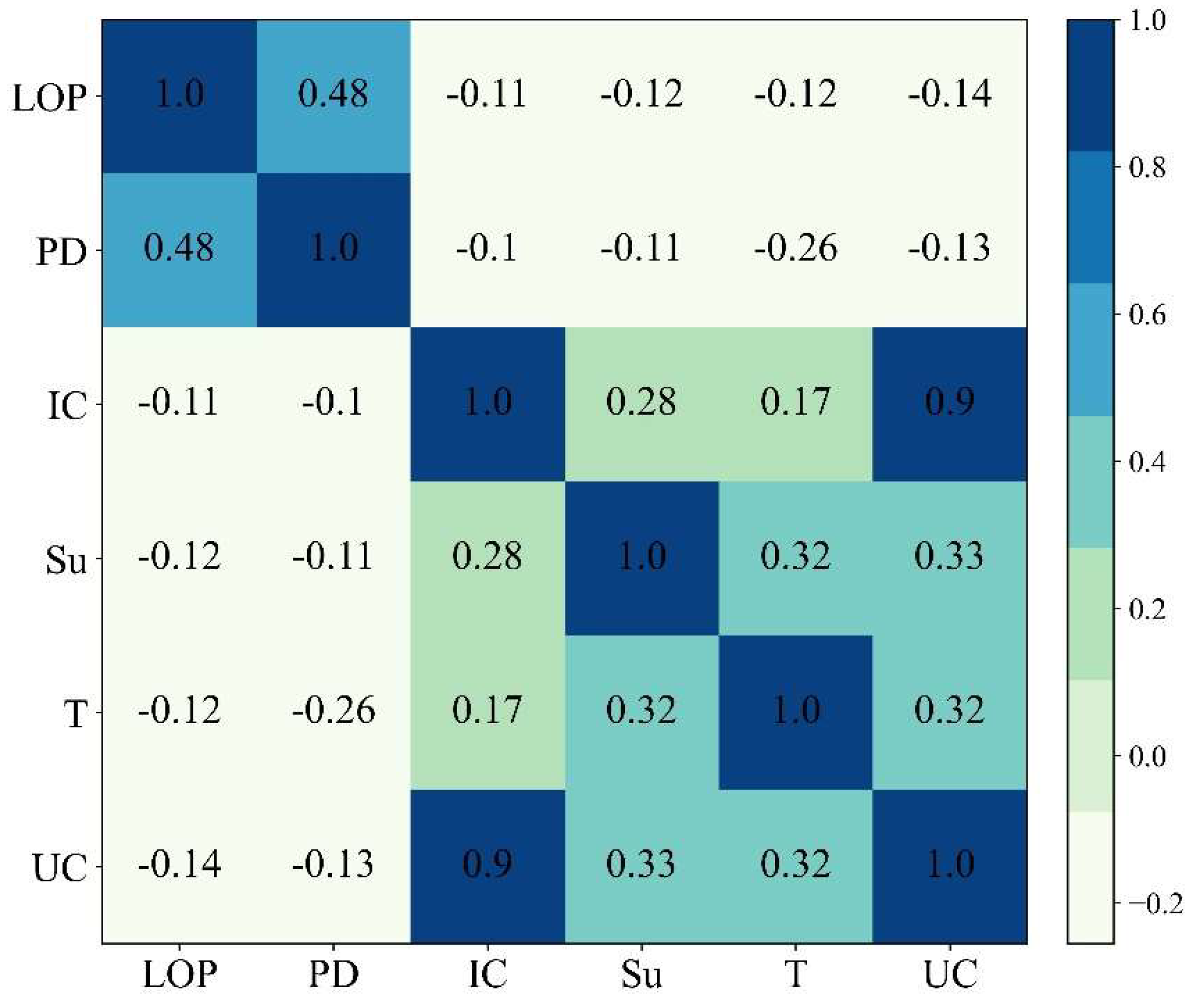
Five relevant factors, including LOP, PD, IC, Su, and T, were measured to build a database for developing the intelligent model to forecast UC. The database is composed of 256 datasets. Statistical analysis was applied to analyze the collected database. Figure 4 presents the boxplots of input and output variables. The box plots are not symmetrical, the database is not a normal distribution, and many data points exceed the upper and lower tentacles of the boxplots. Because the data distribution is unknown, these outliers cannot be eliminated. As shown in Figure 5, Pearson correlation coefficients in Equation (1) between any two variables are calculated [45], and the deeper the color, the stronger the positive correlation, whereas the lighter the color, the stronger the negative correlation. It can be seen that UC has a negative correlation with LOP and PD in five input variables.
where and are variables, and are their mean values, and n is the total number of data points.
4. Prediction of Pile Capacity
4.1. GP Modeling Procedure
In this study, UC correlates with LOP, PD, IC, Su, and T; therefore, UC = f (LOP, IC, PD, Su, and T). GP was implemented to find a function for predicting UC to explore the relationship between UC and the other five input parameters. In this way, an intelligent equation that is easy to implement can be established for predicting pile capacity. The steps to generating the UC prediction formula by GP are as follows:
- (1)
- A training set and a testing set were created by randomly dividing the database. Then, 80 percent of the database (204 datasets) was dedicated to the training set, while the remaining 20 percent was devoted to testing (52 datasets). The initial population is randomly generated from the database and function sets. The function sets include +, −, ×, ÷, , sin, cos, and tan.
- (2)
- The testing set is adapted to fit the prediction equation. After the genetic operation, i.e., selection, crossover, and variation, the preliminary prediction formula is obtained [46].
- (3)
- The fitness function of the population is defined, and it is employed to evaluate the fitness of each formula in the population. Root mean square error (RMSE) as the fitness function was used in this study. The fitness value is calculated according to Equation (2), where M means the number of training or testing sets, and represents the predicted value of the formula generated by GP.
- (4)
- Repeat steps (2–3) until the training time reaches the termination rule.
- (5)
- At the end of GP, the final optimal formula is evaluated from the goodness of fit coefficient between the predicted UC obtained by the formula and the real UC. is calculated according to Equation (3).where represents mean values of the UC.
4.2. Results
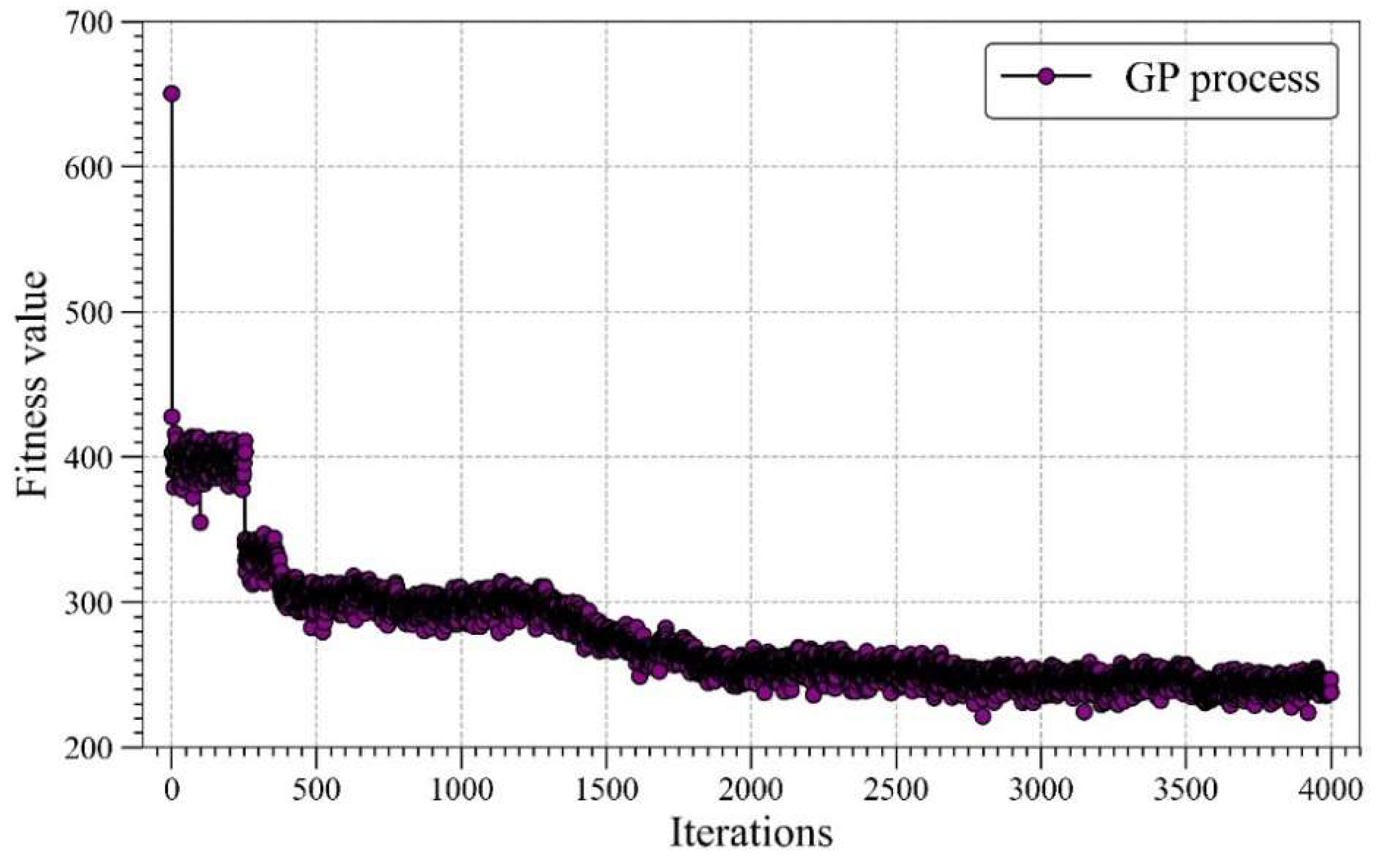
The number of iterations is set to 4000, and Figure 6 exhibits the convergence of fitness values during iterations. When the iteration reaches 2000, the fitness value does not descend. Accordingly, the result returned at the end of the iteration is considered the optimal solution. Figure 7 presents the tree structure of optimal results. The tree structure can be simplified to Equation (4). Equation (4) is the final equation developed by GP to estimate the UC.
For evaluating the performance of the developed equation, , RMSE, mean absolute error (MAE), variance account for (VAF), and A-20 index were introduced to evaluate the performance of Equation (4) in training and testing sets [46,47,48,49]. Equations (5)–(7) display the calculation equations for MAE, VAF, and A-20 index, respectively. When the MAE gets closer to 0, the model has better accuracy. When the VAF reaches 100, the predicted UC is perfectly equated to the actual. When the predicted UC is equal to the actual UC, the A-20 index is 1.
where means the variance, and is the number of samples with a ratio of the predicted value to the actual value in the range (0.8–1.2).
Figure 8 shows the predicted results and five regression indicators in training and testing tests. When the predicted UC equals the true UC, the corresponding point falls on the red line in the figure. The points falling between the two purple dotted lines indicate that the ratio of the predicted UC to the real UC is between 0.8 and 1.2. The A-20 index indicates that some of the predicted values are different from the actual values.
5. Optimizing Pile Capacity Using Metaheuristic Algorithms
5.1. Gray Wolf Optimization
In the last section, the performance of the developed equation is evaluated. Some optimization techniques have been introduced to maximize Equation (4) to improve the UC. GWO was implemented to find the maximum UC. To perform GWO, an open-source Python library, Mealpy, was applied [50]. The main parameters of GWO used the default parameters in Mealpy. To see more about how to implement GWO in Python, the reference [50] used in this study is useful.
Before optimization modeling, the range of parameters needs to be determined. As shown in Table 1, the input range of five parameters was selected as the optimization range. The maximum UC is found in the range. The swarm is set to 50, 100, 150, and 250 [22]. Figure 9 shows the fitness variation during GWO. When the swarm is 50, the found UC is the maximum. When LOP is 38.59, PD is 0.247, IC is 2273, Su is 157.46, T is 153.18, the maximum UC is 6098.488.
5.2. Artificial Bee Colony Algorithm
ABC was also implemented to compare optimization techniques to find the maximum UC in Equation (4). The default parameters suggested in Mealpy [50] were also considered in this study to construct an ABC optimization model. The optimization range used the parameters range in Table 1. The swarm is set to 50, 100, 150, and 250. Figure 10 shows the fitness variation during the process of ABC. When the swarm is set to 100, 150, and 200, the found UC is the maximum. When LOP is 38.47, PD is 0.240, IC is 2276, Su is 157.46, and T is 170.16, the maximum UC is 6043.64. It is apparent that GWO performs better than ABC in finding the maximum UC.
6. Discussion
GP was adopted to develop the equation for predicting the UC, and the developed equation received of 0.897 in the training set and of 0.844 in the testing set. Five regressions revealed that the developed equation can better forecast the UC than previous methods. To analyze the strength of GP for predicting UC, some other widely used machine learning models were also developed to build intelligent models for predicting UC. These widely used models include random forest (RF), gradient boosting machine (GBM), adaptive boosting machine (AdaBoost), ANN, support vector machine (SVM), k-nearest neighbor (KNN), and decision tree (DT). These models were developed according to the default parameters in Scikit-learn [51].
These models were developed using the training set, and the testing set was used to evaluate their performance. An easy way to compare the results of several modeling approaches is to use a Taylor diagram. The Taylor diagram cleverly combines the correlation coefficient, the centered RMSE, and the standard deviation into a polar diagram as a result of these inputs. A cosine connection [52] may be seen in Equation (8) between the correlation coefficient, the center RMSE, and the standard deviation.
In Equation (8), is the centered RMSE between measured and predicted parameters, is the variance of predicted parameters, is the variance of measured parameters, and is the correlation coefficient between measured and predicted parameters.
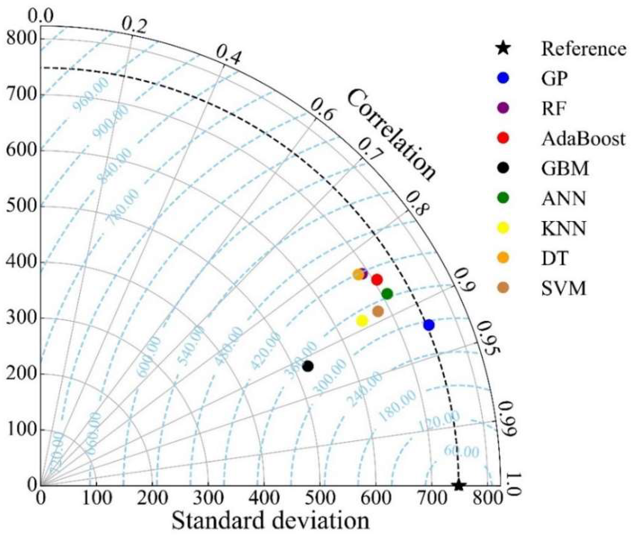
The Taylor diagrams for the training and testing sets are shown in Figure 11 and Figure 12, respectively. The closer the model is to the reference point, the smaller the centered RMSE of the model, the higher the correlation coefficient between the prediction results and the actual results, and the better performance of the model. According to this graph, a model’s performance improves as it gets closer to its associated “Reference” point. It can be found that GP has outstanding performance during the training and testing stages.
Additionally, GWO and ABC were implemented to find the maximum UC. Table 2 shows the optimized parameters. The GWO performs better than ABC. The maximum UC found by GWO is 6089.488, which is an increase of 54% compared to the maximum UC in this database. The maximum UC found by ABC is 6043.64, which is an increase of 52.6% compared to the maximum UC in this database. It is apparent that using the optimized parameters can improve UC.
7. Limitations and Future Works
According to the previous research on this subject, it is essential to consider that other variables may have a profound impact on the prediction process of pile setup, such as coefficient of consolidation, or over consolidation ratio, which have not been considered in this study due to the lack of appropriate data sets. In addition, to make these types of studies more informative for civil engineers, previous empirical equations or developed theories in the area of pile capacity can be considered and used in the portion of data preparation. In this way, a civil engineer or a geotechnical engineer has enough knowledge regarding data preparation. A combination of these theories together with AI models makes these types of studies different and more applicable than an application of AI methodologies. The proposed techniques in both the prediction and optimization phases of this study were constructed based on the entire database described in Section 3 and are valid in the range of this database. The results may be different if out-of-range inputs are used.
8. Conclusions
A different view regarding the common pile capacity studies was considered in this study. To evaluate the effect of the soil setup on the pile bearing capacity over time, an intelligent equation using a GP model was proposed. To develop the prediction models, a comprehensive database obtained from some geotechnical projects carried out in Mahshahr, Iran, was used. In addition, a new section, namely optimization, has been proposed for maximizing the bearing capacity. The following conclusions and remarks can be drawn from this study:
- The proposed GP equation is easy to implement and is of interest to civil and geotechnical engineers. An intelligent equation proposed by GP showed an acceptable level of accuracy in predicting pile capacity. Results with values of 0.897 in the training stage and 0.844 in the testing stage indicate that this GP model is capable enough to be implemented for predicting pile capacity.
- In the optimization phase, two powerful algorithms, namely GWO and ABC, were applied to maximize pile capacity. Obtaining the highest capacity of the pile is considered the ultimate objective of such projects. Although both algorithms are powerful in maximizing pile capacity, GWO performed better. Increase percentages of 52.6 and 54 were obtained by ABC and GWO, respectively, in their pile capacity results.
- For the best optimization algorithm (i.e., GWO), values of 38.59 m, 0.247 m, 2273 kPa, 157.46 kPa, 153.18 days, and 6098.488 kPa were obtained for LOP, PD, IC, Su, T, and UC, respectively. The proposed models and obtained results of this study can be used in designing pile capacity before implementing relevant projects.
Author Contributions
M.K.: conceptualization, methodology, investigation, writing—original draft preparation, writing—review and editing. D.J.A.: conceptualization, methodology, investigation, formal analysis, writing—original draft preparation, writing—review and editing, supervision. M.M.S.S.: writing—original draft preparation, writing—review and editing, supervision, funding acquisition. All authors have read and agreed to the published version of the manuscript.
Funding
The research is partially funded by the Ministry of Science and Higher Education of the Russian Federation under the strategic academic leadership program ‘Priority 2030’ (Agreement 075-15-2021-1333 dated 30 September 2021).
Data Availability Statement
Data is available upon request.
Conflicts of Interest
The authors declare no conflict of interest.
References
- Titi, H.H.; Wije Wathugala, G. Numerical procedure for predicting pile capacity—Setup/freeze. Transp. Res. Rec. 1999, 1663, 25–32. [Google Scholar] [CrossRef]
- Roy, M.; Blanchet, R.; Tavenas, F.; Rochelle, P. La Behaviour of a sensitive clay during pile driving. Can. Geotech. J. 1981, 18, 67–85. [Google Scholar] [CrossRef]
- Fakharian, K.; Khanmohammadi, M. Comparison of pile bearing capacity from CPT and dynamic load tests in clay considering soil setup. In Frontiers in Offshore Geotechnics III; CRC Press: Boca Raton, FL, USA, 2015; pp. 539–544. [Google Scholar]
- Khanmohammadi, M.; Fakharian, K. Evaluation of performance of piled-raft foundations on soft clay: A case study. Geomech. Eng. 2018, 14, 43–50. [Google Scholar]
- Komurka, V.E.; Wagner, A.B.; Edil, T.B. Estimating Soil/Pile Set-Up; Wisconsin Highway Research Program: Madison, WI, USA, 2003. [Google Scholar]
- Abu-Farsakh, M.Y.; Haque, M.N. Estimation and Incorporation of Pile Setup into LRFD Design Methodology. In Proceedings of the Transportation Research Board 97th Annual Meeting, Washington, DC, USA, 7–11 January 2018. [Google Scholar]
- Abu-Farsakh, M.Y.; Haque, M.N.; Tavera, E.; Zhang, Z. Evaluation of pile setup from osterberg cell load tests and its cost–benefit analysis. Transp. Res. Rec. 2017, 2656, 61–70. [Google Scholar] [CrossRef]
- Haque, M.N.; Steward, E.J. Evaluation of pile setup phenomenon for driven piles in Alabama. In Geo-Congress 2020: Foundations, Soil Improvement, and Erosion; American Society of Civil Engineers: Reston, VA, USA, 2020; pp. 200–208. [Google Scholar]
- Lanyi-Bennett, S.A.; Deng, L. Effects of inter-helix spacing and short-term soil setup on the behaviour of axially loaded helical piles in cohesive soil. Soils Found. 2019, 59, 337–350. [Google Scholar] [CrossRef]
- Khanmohammadi, M.; Fakharian, K. Numerical modelling of pile installation and set-up effects on pile shaft capacity. Int. J. Geotech. Eng. 2017, 13, 484–498. [Google Scholar] [CrossRef]
- Fakharian, K.; Khanmohammadi, M. Effect of OCR and Pile Diameter on Load Movement Response of Piles Embedded in Clay over Time. Int. J. Geomech. 2022, 22, 04022091. [Google Scholar] [CrossRef]
- Bogard, J.D.; Matlock, H. Application of model pile tests to axial pile design. In Proceedings of the Offshore Technology Conference, Houston, TX, USA, 7–10 May 1990. [Google Scholar]
- Yan, W.M.; Yuen, K. V Prediction of pile set-up in clays and sands. In IOP Conference Series: Materials Science and Engineering; IOP Publishing: Bristol, UK, 2010; Volume 10, p. 12104. [Google Scholar]
- Skov, R.; Denver, H. Time-dependence of bearing capacity of piles. In Proceedings of the Third International Conference on the Application of Stress-Wave Theory to Piles, Ottawa, ON, Canada, 25–27 May 1988; pp. 25–27. [Google Scholar]
- Gardner, M.W.; Dorling, S.R. Artificial neural networks (the multilayer perceptron)—A review of applications in the atmospheric sciences. Atmos. Environ. 1998, 32, 2627–2636. [Google Scholar] [CrossRef]
- Parsajoo, M.; Armaghani, D.J.; Mohammed, A.S.; Khari, M.; Jahandari, S. Tensile strength prediction of rock material using non-destructive tests: A comparative intelligent study. Transp. Geotech. 2021, 31, 100652. [Google Scholar] [CrossRef]
- Hasanipanah, M.; Monjezi, M.; Shahnazar, A.; Armaghani, D.J.; Farazmand, A. Feasibility of indirect determination of blast induced ground vibration based on support vector machine. Measurement 2015, 75, 289–297. [Google Scholar] [CrossRef]
- Li, D.; Liu, Z.; Armaghani, D.J.; Xiao, P.; Zhou, J. Novel Ensemble Tree Solution for Rockburst Prediction Using Deep Forest. Mathematics 2022, 10, 787. [Google Scholar] [CrossRef]
- Koopialipoor, M.; Asteris, P.G.; Mohammed, A.S.; Alexakis, D.E.; Mamou, A.; Armaghani, D.J. Introducing stacking machine learning approaches for the prediction of rock deformation. Transp. Geotech. 2022, 34, 100756. [Google Scholar] [CrossRef]
- De-Prado-Gil, J.; Zaid, O.; Palencia, C.; Martínez-García, R. Prediction of Splitting Tensile Strength of Self-Compacting Recycled Aggregate Concrete Using Novel Deep Learning Methods. Mathematics 2022, 10, 2245. [Google Scholar] [CrossRef]
- Barkhordari, M.; Armaghani, D.; Asteris, P. Structural Damage Identification Using Ensemble Deep Convolutional Neural Network Models. Comput. Model. Eng. Sci. 2022, 134, 2. [Google Scholar] [CrossRef]
- Zhou, J.; Qiu, Y.; Khandelwal, M.; Zhu, S.; Zhang, X. Developing a hybrid model of Jaya algorithm-based extreme gradient boosting machine to estimate blast-induced ground vibrations. Int. J. Rock Mech. Min. Sci. 2021, 145, 104856. [Google Scholar] [CrossRef]
- Zhou, J.; Li, X.; Mitri, H.S. Classification of rockburst in underground projects: Comparison of ten supervised learning methods. J. Comput. Civ. Eng. 2016, 30, 4016003. [Google Scholar] [CrossRef]
- Zhou, J.; Chen, C.; Wang, M.; Khandelwal, M. Proposing a novel comprehensive evaluation model for the coal burst liability in underground coal mines considering uncertainty factors. Int. J. Min. Sci. Technol. 2021, 31, 799–812. [Google Scholar] [CrossRef]
- Zhou, J.; Shen, X.; Qiu, Y.; Li, E.; Rao, D.; Shi, X. Improving the efficiency of microseismic source locating using a heuristic algorithm-based virtual field optimization method. Geomech. Geophys. Geo-Energy Geo-Resour. 2021, 7, 89. [Google Scholar] [CrossRef]
- Liu, Z.; Armaghani, D.J.; Fakharian, P.; Li, D.; Ulrikh, D.V.; Orekhova, N.N.; Khedher, K.M. Rock Strength Estimation Using Several Tree-Based ML Techniques. Comput. Model. Eng. Sci. 2022, 133, 3. [Google Scholar] [CrossRef]
- Yang, H.; Wang, Z.; Song, K. A new hybrid grey wolf optimizer-feature weighted-multiple kernel-support vector regression technique to predict TBM performance. Eng. Comput. 2020, 38, 2469–2485. [Google Scholar] [CrossRef]
- Yang, H.; Song, K.; Zhou, J. Automated Recognition Model of Geomechanical Information Based on Operational Data of Tunneling Boring Machines. Rock Mech. Rock Eng. 2022, 55, 1499–1516. [Google Scholar] [CrossRef]
- Kardani, N.; Bardhan, A.; Samui, P.; Nazem, M.; Asteris, P.G.; Zhou, A. Predicting the thermal conductivity of soils using integrated approach of ANN and PSO with adaptive and time-varying acceleration coefficients. Int. J. Therm. Sci. 2022, 173, 107427. [Google Scholar] [CrossRef]
- Baziar, M.H.; Saeedi Azizkandi, A.; Kashkooli, A. Prediction of pile settlement based on cone penetration test results: An ANN approach. KSCE J. Civ. Eng. 2015, 19, 98–106. [Google Scholar] [CrossRef]
- Alkroosh, I.; Nikraz, H. Predicting pile dynamic capacity via application of an evolutionary algorithm. Soils Found. 2014, 54, 233–242. [Google Scholar] [CrossRef]
- Khari, M.; Armaghani, D.J.; Dehghanbanadaki, A. Prediction of Lateral Deflection of Small-Scale Piles Using Hybrid PSO–ANN Model. Arab. J. Sci. Eng. 2020, 45, 3499–3509. [Google Scholar] [CrossRef]
- Armaghani, D.J.; Harandizadeh, H.; Momeni, E.; Maizir, H.; Zhou, J. An optimized system of GMDH-ANFIS predictive model by ICA for estimating pile bearing capacity. Artif. Intell. Rev. 2021, 55, 2313–2350. [Google Scholar] [CrossRef]
- Lee, I.-M.; Lee, J.-H. Prediction of pile bearing capacity using artificial neural networks. Comput. Geotech. 1996, 18, 189–200. [Google Scholar] [CrossRef]
- Shahin, M.A. Intelligent computing for modeling axial capacity of pile foundations. Can. Geotech. J. 2010, 47, 230–243. [Google Scholar] [CrossRef]
- Samui, P. Prediction of pile bearing capacity using support vector machine. Int. J. Geotech. Eng. 2011, 5, 95–102. [Google Scholar] [CrossRef]
- Momeni, E.; Nazir, R.; Armaghani, D.J.; Maizir, H. Prediction of pile bearing capacity using a hybrid genetic algorithm-based ANN. Measurement 2014, 57, 122–131. [Google Scholar] [CrossRef]
- Dehghanbanadaki, A.; Khari, M.; Amiri, S.T.; Armaghani, D.J. Estimation of ultimate bearing capacity of driven piles in c-φ soil using MLP-GWO and ANFIS-GWO models: A comparative study. Soft Comput. 2021, 25, 4103–4119. [Google Scholar] [CrossRef]
- Koza, J.R.; Poli, R. Genetic programming. In Search Methodologies; Springer: Berlin/Heidelberg, Germany, 2005; pp. 127–164. [Google Scholar]
- Koza, J.R.; Koza, J.R. Genetic Programming: On the Programming of Computers by Means of Natural Selection; MIT Press: Cambridge, MA, USA, 1992; Volume 1, ISBN 0262111705. [Google Scholar]
- Mirjalili, S.; Mirjalili, S.M.; Lewis, A. Grey wolf optimizer. Adv. Eng. Softw. 2014, 69, 46–61. [Google Scholar] [CrossRef]
- Faris, H.; Aljarah, I.; Al-Betar, M.A.; Mirjalili, S. Grey wolf optimizer: A review of recent variants and applications. Neural Comput. Appl. 2018, 30, 413–435. [Google Scholar] [CrossRef]
- Karaboga, D. An Idea Based on Honey Bee Swarm for Numerical Optimization; Technical Report-tr06; Erciyes University, Engineering Faculty, Computer Engineering Department: Kayseri, Turkey, 2005. [Google Scholar]
- Karaboga, D. Artificial bee colony algorithm. Scholarpedia 2010, 5, 6915. [Google Scholar] [CrossRef]
- Schober, P.; Boer, C.; Schwarte, L.A. Correlation coefficients: Appropriate use and interpretation. Anesth. Analg. 2018, 126, 1763–1768. [Google Scholar] [CrossRef]
- Armaghani, D.J.; Asteris, P.G. A comparative study of ANN and ANFIS models for the prediction of cement-based mortar materials compressive strength. Neural Comput. Appl. 2020, 33, 4501–4532. [Google Scholar] [CrossRef]
- Zeng, J.; Asteris, P.G.; Mamou, A.P.; Mohammed, A.S.; Golias, E.A.; Armaghani, D.J.; Faizi, K.; Hasanipanah, M. The Effectiveness of Ensemble-Neural Network Techniques to Predict Peak Uplift Resistance of Buried Pipes in Reinforced Sand. Appl. Sci. 2021, 11, 908. [Google Scholar] [CrossRef]
- Mahmood, W.; Mohammed, A.S.; Asteris, P.G.; Kurda, R.; Armaghani, D.J. Modeling Flexural and Compressive Strengths Behaviour of Cement-Grouted Sands Modified with Water Reducer Polymer. Appl. Sci. 2022, 12, 1016. [Google Scholar] [CrossRef]
- Murlidhar, B.R.; Nguyen, H.; Rostami, J.; Bui, X.; Armaghani, D.J.; Ragam, P.; Mohamad, E.T. Prediction of flyrock distance induced by mine blasting using a novel Harris Hawks optimization-based multi-layer perceptron neural network. J. Rock Mech. Geotech. Eng. 2021, 13, 1413–1427. [Google Scholar] [CrossRef]
- Van Thieu, N. A collection of the State-of-the-Art Meta-Heuristics Algorithms in Python: Mealpy; Zenodo: Genève, Switzerland, 2020. [Google Scholar]
- Pedregosa, F.; Varoquaux, G.; Gramfort, A.; Michel, V.; Thirion, B.; Grisel, O.; Blondel, M.; Prettenhofer, P.; Weiss, R.; Dubourg, V. Scikit-learn: Machine learning in Python. J. Mach. Learn. Res. 2011, 12, 2825–2830. [Google Scholar]
- Taylor, K.E. Taylor Diagram Primer; PCMDI: Livermore, CA, USA, 2005. [Google Scholar]
Figure 1.
The flowchart of GP.

Figure 2.
The process of GWO.

Figure 3.
The process of ABC.

Figure 4.
Six input parameters and their box plots.

Figure 5.
The heatmap of inputs and their correlations.

Figure 6.
The value of fitness function during iterations.

Figure 7.
Tree structure representation of optimal results (X0 = LOP; X1 = PD; X2 = IC; X3 = Su; X4 = T).
Figure 7.
Tree structure representation of optimal results (X0 = LOP; X1 = PD; X2 = IC; X3 = Su; X4 = T).

Figure 8.
The performance of equation developed by GP in training and testing sets.

Figure 9.
The fitness variation in GWO.

Figure 10.
The fitness variation in ABC.

Figure 11.
Taylor diagram of training set (RF: random forest, ANN: artificial neural network, DT: decision tree, SVM: support vector machine, KNN: k-nearest neighbors, GBM: gradient boosting machine, AdaBoost: adaptive boosting machine).
Figure 11.
Taylor diagram of training set (RF: random forest, ANN: artificial neural network, DT: decision tree, SVM: support vector machine, KNN: k-nearest neighbors, GBM: gradient boosting machine, AdaBoost: adaptive boosting machine).

Figure 12.
Taylor diagram of the test set (RF: random forest, ANN: artificial neural network, DT: decision tree, SVM: support vector machine, KNN: k-nearest neighbors, GBM: gradient boosting machine, AdaBoost: adaptive boosting machine).
Figure 12.
Taylor diagram of the test set (RF: random forest, ANN: artificial neural network, DT: decision tree, SVM: support vector machine, KNN: k-nearest neighbors, GBM: gradient boosting machine, AdaBoost: adaptive boosting machine).


Table 1.
The input parameters range.
| Parameters | Range |
|---|---|
| LOP | 12.009–64.008 |
| PD | 0.236–1.067 |
| IC | 57.3–2276 |
| Su | 26.97–191.52 |
| T | 0.008–154 |
Table 2.
Optimized values of input parameters for the maximum UC.
| Parameter | Actual Value | Optimized Value | |
|---|---|---|---|
| GWO | ABC | ||
| LOP | 24.0 | 38.59 | 38.47 |
| PD | 0.457 | 0.247 | 0.240 |
| IC | 1642.7 | 2273 | 2276 |
| Su | 172.0 | 157.46 | 157.46 |
| T | 6.0 | 153.18 | 170.16 |
| Maximum UC | 3960.0 | 6098.488 | 6043.64 |
Publisher’s Note: MDPI stays neutral with regard to jurisdictional claims in published maps and institutional affiliations. |
© 2022 by the authors. Licensee MDPI, Basel, Switzerland. This article is an open access article distributed under the terms and conditions of the Creative Commons Attribution (CC BY) license (https://creativecommons.org/licenses/by/4.0/).
Share and Cite
MDPI and ACS Style
Khanmohammadi, M.; Armaghani, D.J.; Sabri Sabri, M.M. Prediction and Optimization of Pile Bearing Capacity Considering Effects of Time. Mathematics 2022, 10, 3563. https://doi.org/10.3390/math10193563
AMA Style
Khanmohammadi M, Armaghani DJ, Sabri Sabri MM. Prediction and Optimization of Pile Bearing Capacity Considering Effects of Time. Mathematics. 2022; 10(19):3563. https://doi.org/10.3390/math10193563
Chicago/Turabian StyleKhanmohammadi, Mohammadreza, Danial Jahed Armaghani, and Mohanad Muayad Sabri Sabri. 2022. "Prediction and Optimization of Pile Bearing Capacity Considering Effects of Time" Mathematics 10, no. 19: 3563. https://doi.org/10.3390/math10193563
Note that from the first issue of 2016, this journal uses article numbers instead of page numbers. See further details here.