Article

Modeling the Nonlinearity of Sea Level Oscillations in the Malaysian Coastal Areas Using Machine Learning Algorithms

1
Department of Civil Engineering, College of Engineering, Universiti Tenaga Nasional (UNITEN), Kajang 43000, Selangor Darul Ehsan, Malaysia
2
Institute for Energy Infrastructure (IEI), Universiti Tenaga Nasional (UNITEN), Kajang 43000, Selangor Darul Ehsan, Malaysia
3
Institute of Sustainable Energy (ISE), Universiti Tenaga Nasional (UNITEN), Kajang 43000, Selangor Darul Ehsan, Malaysia
4
Department of Civil Engineering, Faculty of Engineering, University of Malaya (UM), Kuala Lumpur 50603, Malaysia
5
Civil Engineering Department, Giza Higher Institute for Engineering and Technology, Giza, Egypt
*
Authors to whom correspondence should be addressed.
Sustainability 2019, 11(17), 4643; https://doi.org/10.3390/su11174643
Submission received: 3 June 2019 / Revised: 11 July 2019 / Accepted: 18 July 2019 / Published: 26 August 2019
(This article belongs to the Special Issue Sustainable Development of Seaports)

Abstract

:
The estimation of an increase in sea level with sufficient warning time is important in low-lying regions, especially in the east coast of Peninsular Malaysia (ECPM). This study primarily aims to investigate the validity and effectiveness of the support vector machine (SVM) and genetic programming (GP) models for predicting the monthly mean sea level variations and comparing their prediction accuracies in terms of the model performances. The input dataset was obtained from Kerteh, Tioman Island, and Tanjung Sedili in Malaysia from January 2007 to December 2017 to predict the sea levels for five different time periods (1, 5, 10, 20, and 40 years). Further, the SVM and GP models are subjected to preprocessing to obtain optimal performance. The tuning parameters are generalized for the optimal input designs (SVM2 and GP2), and the results denote that SVM2 outperforms GP with R of 0.81 and 0.86 during the training and testing periods, respectively, at the study locations. However, GP can provide values of 0.71 and 0.79 for training and testing, respectively, at the study locations. The results show precise predictions of the monthly mean sea level, denoting the promising potential of the used models for performing sea level data analysis.

1. Introduction

An increase in sea level will considerably impact the low-lying coastal regions and increase the risk of floods [1,2,3,4]. In Malaysia, the low-lying coastal regions host very large cities and are densely populated. Therefore, the future increase in sea level should be comprehensively analyzed to protect the low-lying residential regions and coastal areas [5,6,7,8,9].
Various methods have been introduced for predicting the sea level increase [10,11]. These methods have been developed based on the simple linear production process. Therefore, these methods failed to capture the nonlinearity and complexity associated with the systems [12,13,14,15].
The selection of the appropriate model input considerably influences the model accuracy. The accuracy of the current models used to predict the increase in sea level differs in terms of the prediction horizons (1, 5, 10, 20, and 40 years). Various parameters (rainfall, sea surface temperature, etc.) should be incorporated into these models to improve their performances and successfully reduce the magnitude of uncertainty and prediction error. However, most of these meteorological data are often unavailable [16].
The artificial intelligence techniques have recently gained considerable attention from researchers and have been implemented to overcome the limitations associated with the current models. These techniques have become some of the favorable computational methods for predicting the increase in sea level because they can achieve fast computation using only a few parameters as the input [17,18,19,20]. Support vector machines (SVMs) have recently attracted the interest of many researchers for different prediction scenarios [21,22]. Asefa et al. [23] successfully used the SVM for the prediction of the Sevier River Basin (South-Central Utah, USA) at hourly and seasonal intervals. Lu and Zhang (2006) [24] denoted that the SVM outperformed the ANN) during the prediction of annual runoff. Li et al. (2008) [11] combined the SVM with chaos analysis to predict the runoff. The SVM model uses a sigmoid kernel function that enables the model to solve a quadratic programming problem with linear constraints instead of solving a nonconvex and unconstrained minimization problem similar to that in standard ANN training [24]. Pochwat and Daniel (2018) [25] analyzed the application feasibility of ANNs for the preliminary estimation of the duration of critical rainfalls. The results obtained using the ANN can be applied in the simplified method used for directly estimating the reliable rainfall duration.
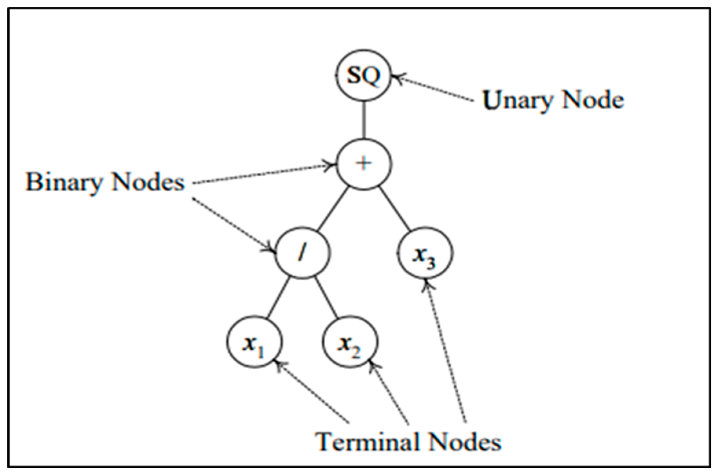
Genetic programming (GP) is a type of evolutionary computational (EC) method, which is a subset of machine learning used to discover solutions to problems that humans have failed to directly solve [26].
Further, the EC techniques can solve difficult problems associated with several different domains, particularly human-competitive machine intelligence [27]. Koza, the father of GP [28], successfully proved the liability of symbolic regression with GP. Optimization is an important subject exhibiting several important applications, and various optimization algorithms have been successfully used for a wide range of applications [29,30]. The most frequently used optimization algorithms include modern metaheuristics, which have introduced a new branch of optimization that can be referred to as metaheuristic optimization.
In GP, a metaheuristic is a condition in which an algorithm is designed for inductive automatic programming and is very suitable for performing the symbolic regression and machine learning tasks. Previous studies have proved that GP can be used as a time series prediction method in various fields. Ghorbani et al. (2010) [31] used GP for forecasting the sea water level at Hillarys Boat Harbor in Western Australia and showed that GP can simulate nonlinear forecasting. The standalone results were then compared with those of the ANN standalone. Consequently, the former was found to perform marginally better for majority of the results. Yan et al. (2019) [32] proposed a hybrid optimized algorithm involving particle swarm optimization (PSO) and genetic algorithm (GA) combined with a BP neural network that can predict the water quality in time series and exhibited a good performance in the Beihai Lake in Beijing. Their study results denoted that the model based on PSO and GA that optimized the BP neural network can predict the water quality parameters with a reasonable accuracy, suggesting that this model is valuable for estimating the quality of lake water. Jonathan and Hatim (2016) [33] focused on modeling the rainfall–runoff relation in a mid-size catchment. As a standalone application, GP was able to outperform the published ANN results obtained using the same dataset, resulting in an average absolute relative error of 17.118 and a Nash–Sutcliffe (E) of 0.937.
The shoreline at the east coast of Peninsular Malaysia (ECPM) is susceptible to direct impacts from severe storms, especially during the northeast monsoon periods. Furthermore, ECPM has a well-established oil refinery offshore structure, a power plant near the shore, and a well-known island with a tourism population. Thus, the increase in sea level rise should be studied to minimize its impact toward these resources at the ECPM.
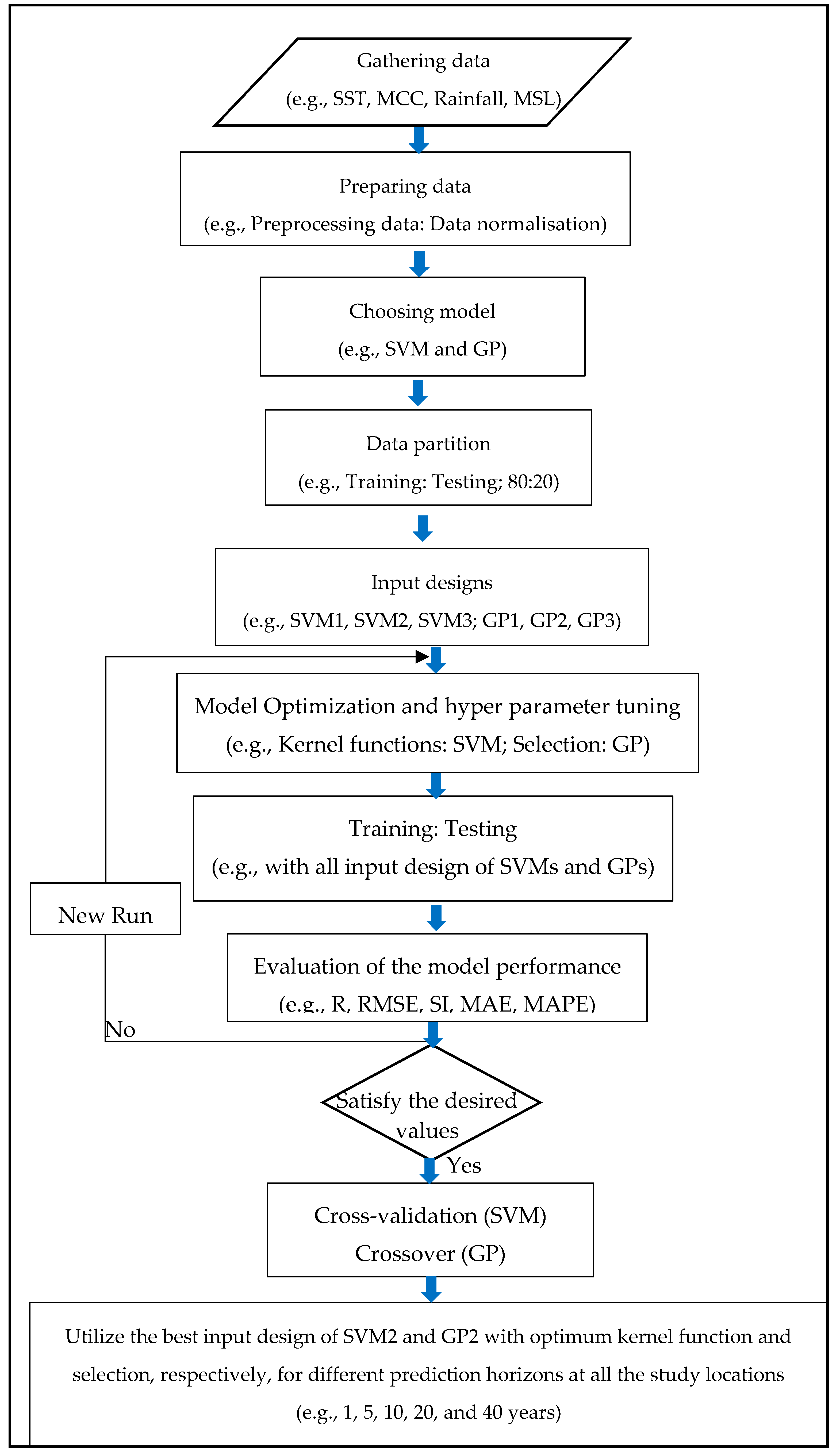
This study implemented two models—SVM and GP—with six different input design parameters. The input design parameters exhibiting a high correlation coefficient were selected for the monthly mean sea level prediction in this study and at two other study locations. Both the model performances were subsequently compared to evaluate their robustness. The highest correlation function kernel and selection of the most optimal input design were executed in different prediction horizons (i.e., 1, 5, 10, 20, and 40 years) [31,32,33] using the two proposed methods.

2. Materials and Methods

2.1. Dataset

Malaysia, which is located in Southeast Asia, comprises the following two noncontiguous regions; Peninsular Malaysia and East Malaysia. Malaysia’s shoreline spans a length of more than 4800 km, and a large portion of this comprises sandy coasts (Figure 1).
The data applied in this study, including the daily minimum and maximum values, sum, average, mean variance, and mean standard deviation (Table 1), were derived based on the longitude and latitude of the three regions in ECPM: Kerteh (longitude: 103.4430° E; latitude: 4.5° N), Tanjung Sedili (longitude: 104.1106° E; latitude: 1.9281° N), and Tioman Island (longitude: 104.1698° E; latitude: 2.7902° N). Subsequently, a total of 396 (11 years × 12 months × 3 regions) historical data related to the monthly mean sea level events were collected. The analyses were conducted according to the Pareto principle (also known as the 80/20 rule) [34] by considering 80% of the obtained data as training data (from January 1, 2007 to December 31, 2015). The remaining 20% was used as testing data (from January 1, 2016 to December 31, 2017) for the SVM and GP models [35,36,37,38]. The historical monthly mean sea level (MMSL) was obtained from the Department of Survey and Mapping Malaysia (DSMM) [39], whereas the historical monthly rainfall data were obtained at a temporal resolution of 3 h with a spatial resolution of a 0.25° latitude–longitude grid from the Tropical Rainfall Measuring Mission (TRMM) satellite [40]. The mean cloud cover was obtained from the Malaysia Meteorological Department. The monthly sea surface temperature (SST) at a spatial grid resolution of 1.0° in latitude–longitude and a temporal resolution of one day [41] were obtained from the website of the National Weather Service, Climate Prediction Centre of National Oceanic and Atmospheric Administration.

2.2. Support Vector Machine

The SVM is an extensively used learning method in both the pattern recognition (classification) and regression problems. Figure 2 denotes the SVM architecture. Further, three different kernels—normalized polynomial kernel, radial basis kernel, and Pearson universal kernel (PUK)—were introduced to train the SVM model for conducting the first assessment and investigate the ability of the SVM model to mimic and learn the preprocessed data.
Normalized polynomial kernel (NP):
k ( x i , x j ) = ( γ x i T · x j + r ) d , γ > 0
Radial basis kernel (RBF):
k ( x i , x j ) = exp ( x i x j 2 ) , γ > 0
Pearson universal kernel (PUK):
k ( x i , x j ) = 1 / [ 1 + ( 2 | x y | 2 2 ( 1 ω ) 1 / σ ) 2 ] ω
The data samples in the NP, Gaussian RBF, and PUK kernels were probably transformed from a high-dimensional space into an infinite-dimensional space, where the data belonging to two categories can be differentiated using a linear hyperplane, because the prediction of the increase in sea level is a nonlinear time series criteria prediction. Hence, the kernel functions were considered for the high-dimensional space Equations (1)–(3) to separate the nonlinear data samples from the linear ones. A suitable kernel function is essential in developing the model to minimize the overfitting or underfitting condition that occurs during the training or testing periods.
K ( x , x i ) = j = 1 m g j ( x ) g j ( x i )
K(xi, xj) is the kernel function. The kernel value is equal to the internal value of two vectors xi and xj in the characteristic spaces ϕ(xi) and ϕ(xj), i.e., K(xi, xj) = ϕ(xi) × ϕ(xj).
Hence, the three kernels were investigated based on the model performance presented in Table 1. The results denoted that the PUK functions were applicable to this work. Thus, the following assessments only focused on the usage of the PUK function for further predicting the MMSL in different prediction horizons because of the robustness of its kernel function.
The SVM generalization performance (estimation accuracy) is renowned to depend on a good setting of the metaparameters C and ε [42,43,44]. C determines the tradeoff between the model complexity (flatness) and degree, whereas ε controls the width of the ε -insensitive zone used to fit the training data. The problem of selecting optimal values for these parameters is further complicated because the SVM model complexity is dependent on the input parameters (e.g., the nonlinearity of the data samples). The metaparameters C and ε were tuned to obtain the most optimal results.
V-fold cross-validation was selected to obtain an almost unbiased estimate of the algorithm performance but with a high variance because, in principle, it can be conducted for as long as one can afford to do so (indicating that it is a trial-and-error method to achieve optimal performances). The models exhibiting outstanding performances were observed when the V-fold was between 7 and 20 [45,46,47].

2.3. Genetic Programming

The GP structure comprised the computer programs represented as expression tress, which are hierarchical, and can dynamically change the size and shape during the evolution process. Figure 3 depicts a typical program that represents ( x 1 x 2 + x 3 ) 2.
GP is a programming model that mimics the biological evolution observed while handling a complex engineering problem. GP is similar to GA in most aspects; they only differ in the structure of searching for a solution. GP employs a “parse tree”, whereas GA employs bite strips [44]. GP contains two components: (i) a parse tree, which is a functional set of basic operators, including {+, −, x,/, ^, log, alog, sin, asin, exp, …}, imitating the role of ribonucleic acid, and (ii) the actual components of the functions and their parameters (referred to as the terminal set), which are obtained in accordance with the role of proteins or chromosomes in biological systems. The mathematical form of such a relation can be given as follows
H t + δ Δ t = ( H t , H t Δ t , H t ω Δ t )
where H denotes the height of the mean sea level with respect to a reference point (m) and δ = 0,1,2, 3…, in which ω describes the time step ( Δ t ) used for predicting the mean sea level.
The evaluation of a GP model is important for denoting its problem solving performance. The fitness function is an explicit evaluation of the GP model. Fitness denotes the evaluation results. The programs for producing the next generation in GP depend on the fitness used to determine the solution [48]. A common fitness measurement is the raw fitness that is known to be stated in the terminology of the problem it explicates as a performance measure [49]. Koza introduced three additional alternative fitness measurements [28]: standardized fitness, adjusted fitness, and normalized fitness. The improved lower numerical value of fitness can be usually presented using standardized fitness, whereas the remaining two are mainly applied for the fitness-proportional selection. The fitness-proportional selection will be investigated in this study.
The fitness function can be presented using a single objective method and a multiobjective method. A single fitness value can be obtained as the output from a single objective fitness function output. With regard to the multiobjective fitness function, multiple weighted values are joined to generate a single fitness value that represents the output [50,51,52,53]. Many studies have recently recommended the usage of the dynamic fitness functions and hierarchically defined fitness functions in GP search [52,54]. The main advantage obtained by proposing the dynamic fitness functions is the simplicity associated with finding an effective fitness function when the problem is mathematically formulated. Therefore, a dynamic fitness function will be used in this study.
The population size and termination criterion are the main parameters that control the GP model. The present algorithm considered a population size of 500, and the number of generations was 300. The proposed values were recommended by other researchers [54,55]. The probability of finding the global optimum increases with a high number of populations and generations by hundreds or more, which could lead to overfitting and underfitting that could influence the prediction accuracy. Hence, after a few trial-and-error attempts, the recommended values were made to function appropriately in this study. Finally, GP was used to compare the accuracy improvement (AI) when compared with that of the SVM (Figure 4).

2.4. Data Normalization and Model Performance

The normalization methods commonly applied include the maximum–minimum, value, and peak methods. The maximum–minimum normalization method will be used herein; the calculations can be given as follows
X j i ^ = X j i X j m i n i X j m a x i X j m i n i
where X j i ^ is the value after normalization, X j i is the value before normalization, X j m a x i is the maximum mean sea level, and X j m i n i is the minimum mean sea level.
Each model was established for different horizons of 1, 5, 10, 20, and 40 years ahead of the sea level prediction such that a comparison of the SVM and GP models can be conducted. Therefore, three different model input parameters were designed to evaluate the improvement in performance prediction because of the various meteorological parameters that were involved. The first parameter is the observation data of the SST and the mean sea level (MSL) data used as the input for SVM1 and GP1 Equation (7). The second parameter is the observed meteorological data of the mean cloud cover (MCC) and rainfall with the SST and MSL data considered to be the input to SVM2 and GP2 Equation (8). In actual situations, the rain gauges may not function because of extreme weather conditions. In these conditions, the SVM3 and GP3 models that use only the MCC, SST, and MSL observations as the input data are alternatives Equation (9). A total of six SVM- and GP-based model algorithms were constructed for different horizons (i.e., 1, 5, 10, 20, and 40 years) before sea level prediction in three different scenarios. The model performances of both the model algorithms were then compared. Table 1 and Table 2 show the results for both, respectively. The comparison between the SVM and GP was further introduced in terms of accuracy improvements and average error percentage to assess the effect of the selected input presented in the results section.
The input designs of the SVM1 and GP1 models can be expressed in the general form as follows
MSLpredicted = (SST + MSL)obs
The input designs of the SVM2 and GP2 models can be expressed in the general form as follows
MSLpredicted = (MSL + SST + Rainfall + MCC)obs
Meanwhile, the input designs of the SVM3 and GP3 models can be expressed in the general form as follows
MSLpredicted = (MSL + SST + MCC)obs
Several criteria can be used to validate the proposed model in this study, which can be given as follows
(i)
The root mean square errors (RMSEs) of the observed and predicted values were compared. The mean absolute error (MAE) is always small or equal to the RMSE. The variance of the individual errors in a sample will increase as long as the difference between the two values increases. Furthermore, all the errors in the sample have the same magnitude if the RMSE is equal to the MAE.
RMSE = i = 1 n ( M S L p M S L o ) 2 N
(ii)
The correlation coefficient (R) was applied to evaluate the relation between variables.
R = i = 1 n ( M S L o M S L ¯ o ) ( M S L p M S L ¯ p ) i = 1 n ( M S L o M S L ¯ o ) 2 i = 1 n ( M S L p M S L ¯ p ) 2
(iii)
The scatter index (SI) was calculated by dividing the RMSE with the mean of the observations.
SI = R M S E x ¯
(iv)
The MAE measures the accuracy of continuous variables.
MAE = 1 n i = 1 N | M S L p M S L o |
(v)
The mean absolute percentage error (MAPE) is the mean or average of the absolute percentage errors associated with forecasts.
MAPE = 100 × [ MAE MSL ¯ p ]
(vi)
AI will be used to measure the significance of the proposed SVM2 over GP2 and can be expressed as follows
AI = S V M 2 G P 2 G P 2 × 100
(vii)
The error percentage is used to determine the prediction precision and can be expressed as follows
EP = M S L p M S L o M S L o × 100 %
where M S L o and M S L p denote the observed and predicted MMSL in the ith month, respectively; n is the number of data; and M S L ¯ o and M S L ¯ p are the mean values of the sea levels and simulation, respectively.

3. Results

This study aimed to examine the capability of the SVM and GP models in different prediction horizons of 1, 5, 10, 20, and 40 years for MMSL forecasting of the sea level in Kerteh, the Tioman Island, and Tanjung Sedili at the EPCM. The results of the study using the SVM in various kernel functions (i.e., NP, RBF, and PUK) and in the GP-based model, namely the ramped half–half (RHH) model with fitness-proportional selection and rank selection, were obtained for comparing the capabilities of the two models.
SVM and GP among different input designs (i.e., SVM1, SVM2, and SVM3 and GP1, GP2, and GP3) were executed to determine the correlation between the input and output of the models by examining the prediction accuracy in terms of the statistical model performance. The input designs of the SVM (SVM1, SVM2, and SVM3) and GP (GP1, GP2, and GP3) were then optimized using different kernel functions of NP, RBF, PUK, and RHH with rank or fitness selection to find the most optimal tuning or affecting parameters for further predicting the horizons.

3.1. Model Performances of the SVM Model

As summarized in Table 3 for Kerteh, for the SVM1 input design based on the combination of the MSL and the SST, the RBF kernel showed an average performance with correlation coefficients of 0.510 and 0.443 for training and testing, respectively. The NP and PUK kernels in SVM1 were not able to perform. In addition, the input designs of SVM3 at Kerteh showed that among the three different kernels, a slight decrease in accuracy was observed in terms of R and RMSE when compared with that observed in the NP and PUK kernels in SVM2. However, R managed to become greater than 0.7 during training. Meanwhile, PUK performed slightly better than NP during testing. However, the RBF performance for the SVM3 input design plummeted when compared with that of SVM2. The model performance was unable to reach a moderate accuracy of R = 0.5 during the testing stage. Furthermore, the SVM2 input design at Kerteh depicted a significant increase in model performance in terms of R, RMSE, SI, MAE, and MAPE. The comparison between the NP and the RBF for the SVM2 input design showed that the NP outperformed the RBF. However, the PUK kernel performed better than the NP kernel.
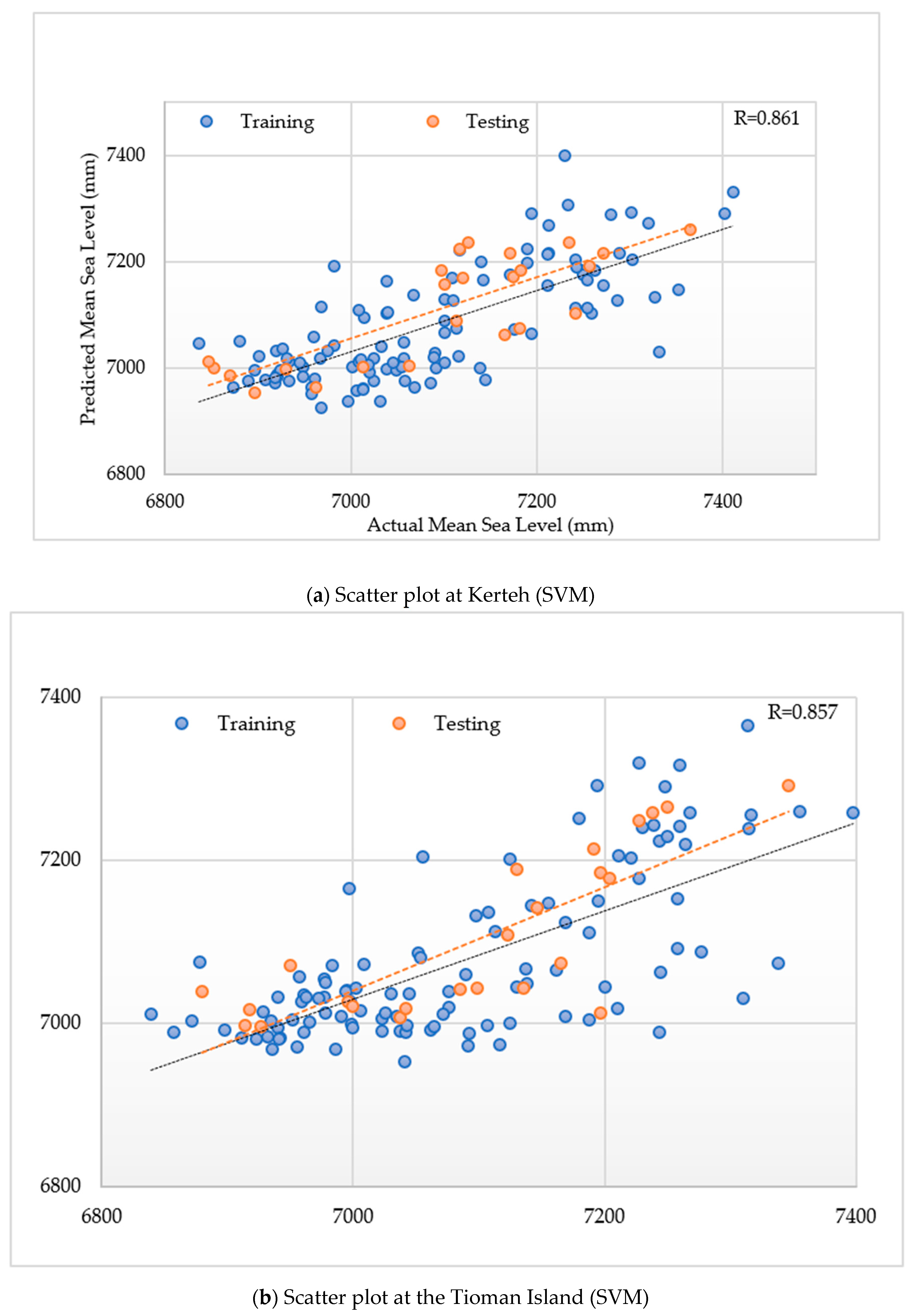
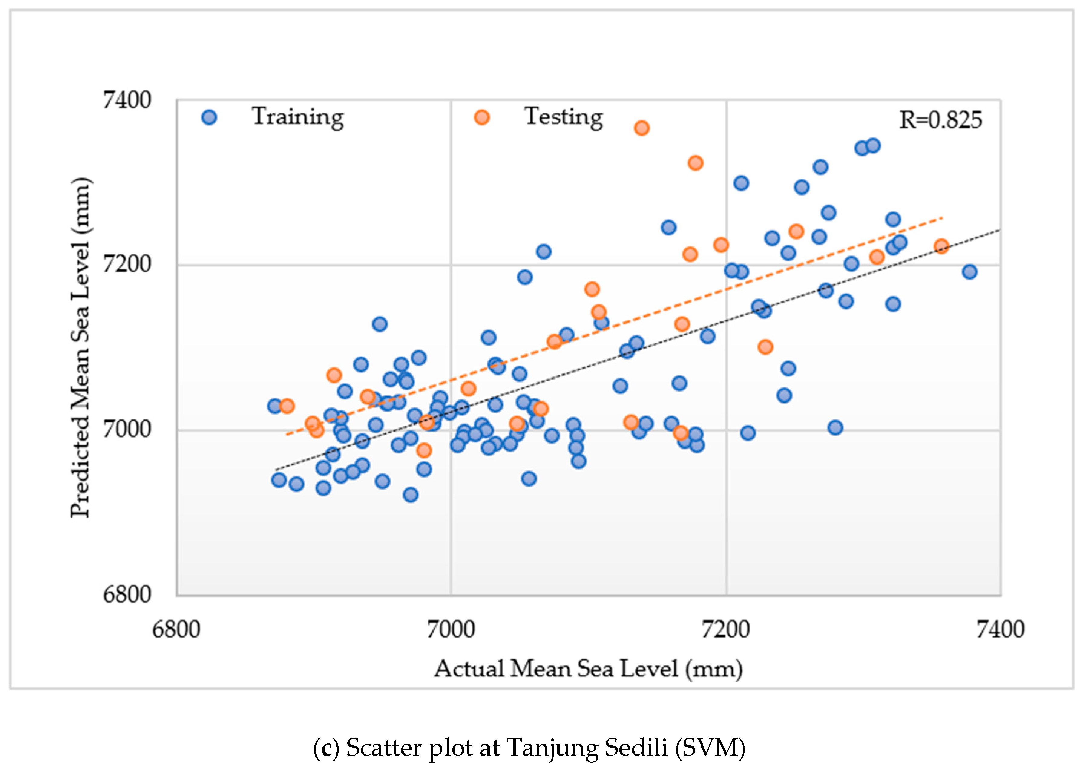
Figure 5a–c present the scatterplots of the actual versus predicted sea levels. The PUK model was capable of precisely mimicking the actual data during the training and testing stages for a 10-year horizon when compared with the remaining different kernels. Hence, the implementation of the PUK function for the proposed SVM models can improve the accuracy. Furthermore, it can be introduced as a perfect substitute model for predicting increases in sea level that are usually nonlinear at several locations along the shoreline. Figure 6 depicts the results in which the PUK fairly accurately performed at three different locations.
The results of the PUK with the SVM2 input design at Kerteh was outperformed other kernel functions. Thus, the Tioman Island and Tanjung Sedili were generalized using the PUK with the SVM2 input design. 
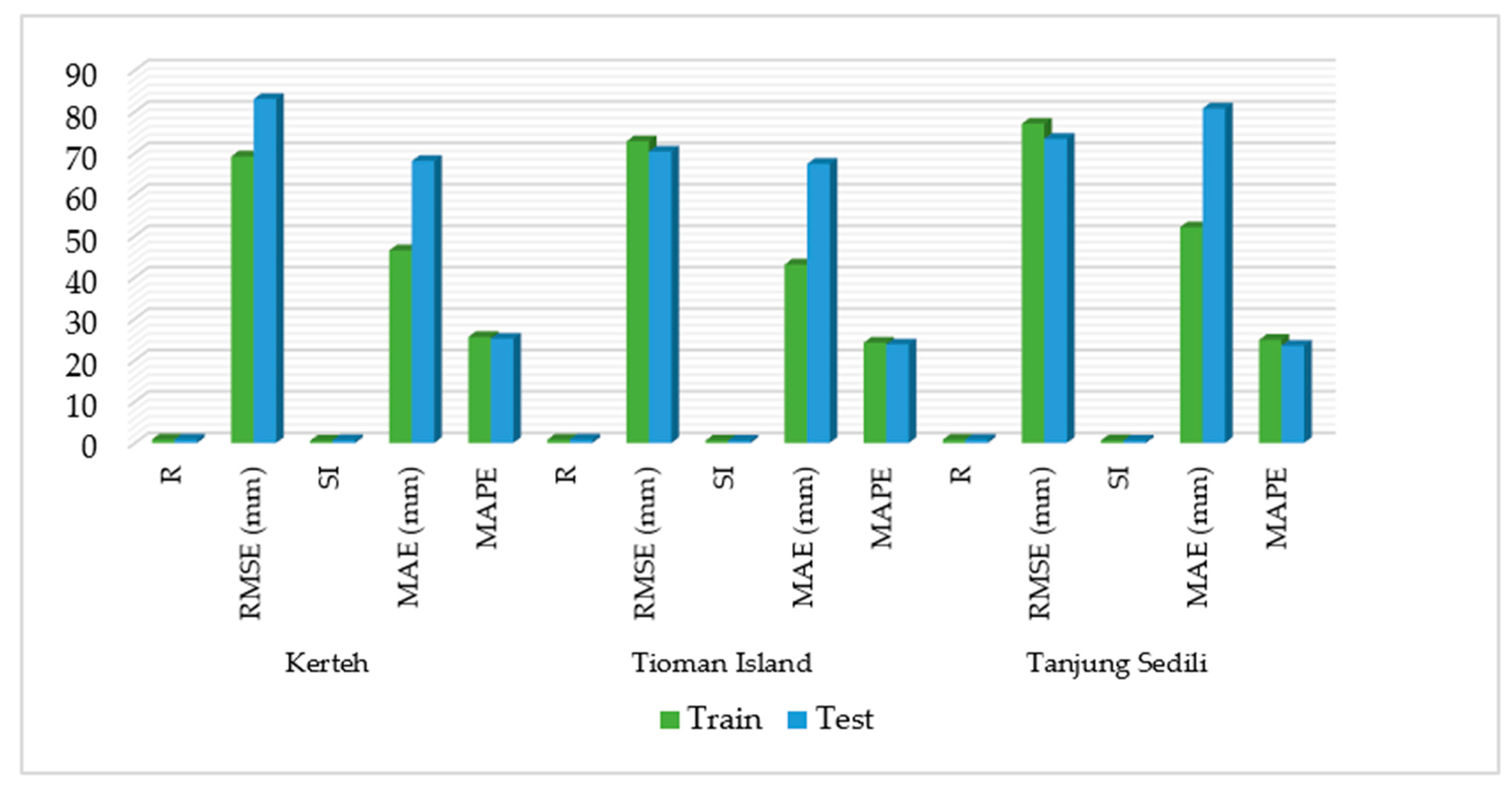
Figure 6 presents the model performances of the R, RMSE, SI, MAE, and MAPE at Kerteh, the Tioman Island, and Tanjung Sedili. The best R performance was 0.820 and 0.857 for the training and testing periods, respectively, at the Tioman Island, whereas the optimal PUK model was observed to be that with minimum RMSE values of 72.83 and 70.34 mm during the training and testing periods, respectively.
In accordance with Figure 6, the PUK was optimal with R of 0.815 and 0.825 for training and testing, respectively, at Tanjung Sedili. The optimal PUK model was clearly the one showing minimum RMSE values of 77.1 and 73.43 mm during the training and testing periods, respectively (Figure 6).
In addition, the model performances of SI for the Tioman Island were 0.61 and 0.58 during the training and testing periods, respectively, whereas those for Tanjung Sedili were 0.64 and 0.611 during the training and testing periods, respectively.
Figure 6 illustrates that the MAE at the Tioman Island is 43.08 and 67.41 mm during the training and testing periods, respectively, and that the MAPE is 24.2% and 23.8% during the training and testing periods, respectively. The MAE at Tanjung Sedili decreased to 52.08 and 80.76 mm during the training and testing periods, respectively. Meanwhile, the MAPE at Tanjung Sedili was 24.9% and 23.5% during the training and testing periods, respectively.

3.2. Optimal Kernel Functions with the Input Design of SVM2 for the Cross-Validation Process

The results for majority of the optimal tuning or affecting parameter settings were obtained in the best kernel function, the PUK with the SVM2 input design for the cross-validation techniques (Table 4). The dataset was divided into two subsets; one subset was assigned to train the models, whereas the other was used to evaluate the performance of the best models.

3.3. Model Performances of GP

The model performances were executed using the input design of GP1 Equation (7). The combination of the MSL and SST could not achieve the best performance in terms of RHH and rank selection because of the lack of accuracy obtained during the testing stage. However, RHH and fitness selection attained a model performance similar to that of GP3. However, both GP1 and GP3 only worked for an alternative purpose, and the optimal model performance from the input design of GP2 was still more convincing.
The input design of GP2 with RHH and fitness selection outperformed the results when compared with the results of half–half and rank selection that exhibited inconsistency of performance during the testing stage with R = 0.45. However, the training results provided a convincible value of R = 0.78 in Figure 6. RHH and fitness selection had the best model performance run in GP2 because of these unstable model selections. Moreover, the optimal RHH with the fitness-proportional selection model had a minimum RMSE value of 89.20 mm during the testing period.
The input design of GP3 for the RHH and fitness functions obtained persuasive model performance results because the combination of the input design of GP3 did not have rainfall input; however, the training and testing stages yielded correlation coefficients of 0.756 and 0.57, respectively, which are considered as above-average and acceptable outcomes if no rainfall data are used as input parameters. The advantage of this combination of GP3 may benefit the impromptu prediction required for coastal management because the model performance did not show a value lower than R = 0.5. Hence, this combination can be an alternative method for predicting the SL.
Table 5 presents the summary of the model performances of the GP with different selections and input designs executed at Kerteh. The model performance was evaluated in terms of R, RMSE, SI, MAE, and MAPE. Throughout the model among the three input designs, the best model performance was obtained from GP2 with RHH and fitness-proportional selection. Hence, the performances of GP2 with RHH and fitness-proportional selection were executed at the Tioman Island and Tanjung Sedili.
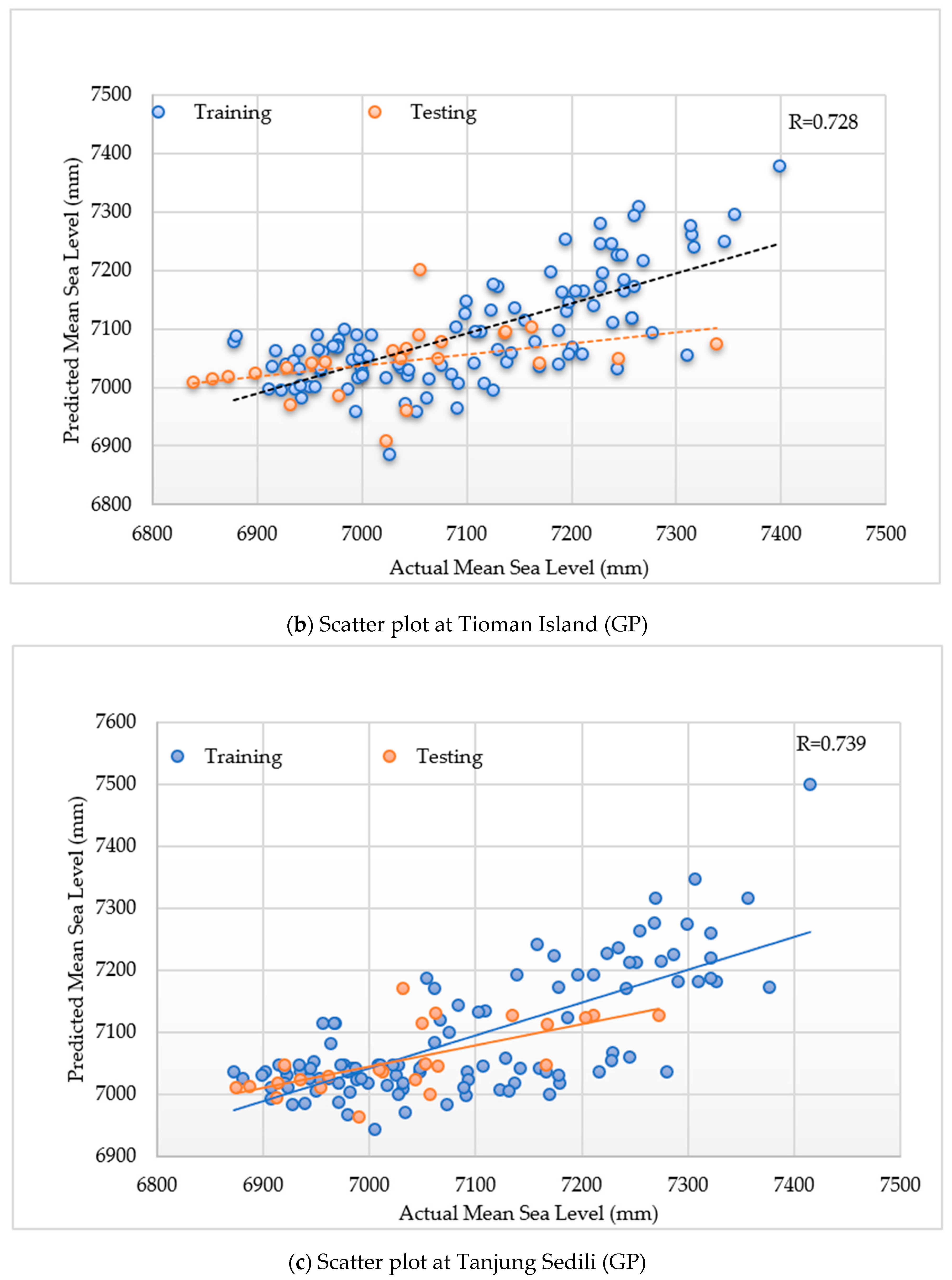
In case of the Tioman Island, the input design of GP2 with RHH and fitness-proportional selection showed R values of 0.712 and 0.728 for the training and testing periods, respectively (Figure 7). Meanwhile, at Tanjung Sedili, the R values were 0.793 and 0.739 for the training and testing periods, respectively.
The input design at Kerteh was outperformed by the RHH and the fitness-proportional selection with GP2. Thus, the Tioman Island and Tanjung Sedili were generalized with the RHH and the fitness-proportional selection with GP2.
Figure 8 shows that the RMSE at the Tioman Island was 90.46 and 84.88 mm during the training and testing periods, respectively, whereas that at Tanjung Sedili was 86.52 and 79.32 mm during the training and testing periods, respectively.
The model performance of SI for the Tioman Island yielded 1.25 and 1.01 for the training and testing periods, respectively, whereas that at Tanjung Sedili yielded 1.29 and 1.05 for the training and testing periods, respectively.
Figure 8 also illustrates that the MAE at the Tioman Island was 101.3 and 97.4 mm for the training and testing periods, respectively, and that the MAPE was 28.2% and 25.4% for the training and testing periods, respectively. The MAE at Tanjung Sedili was 101.5 and 111.2 mm, respectively, and the MAPE was 25.2% and 26.1% for the training and testing periods, respectively.

3.4. Optimal Selection Function with the Input Design of GP2 in the Crossover Process

The crossover operation frequency can be determined by the crossover rate in GP [44]. It is advisable to search for a promising region at the beginning of optimization. The convergence speed decreases with low crossover frequencies. The mutation operation is restrained by the mutation rate. A high population diversity introduced by a high mutation rate may lead to instability. A typical choice of setting the initial GP control parameters would involve the generation run (termination criterion) being fixed at 300 runs to obtain the optimal results and the population being fixed at 500 [42]. These control parameters were managed to match the input data design, and the capability of the model was good (Table 6).

3.5. Comparison of the Average Error Percentages in SVM2 and GP2 at the Study Locations

Figure 9 illustrates a comparison of the SVM2 and GP2 average error percentages of both models at Kerteh, the Tioman Island, and Tanjung Sedili. Figure 8 demonstrates the fluctuation trendline for both the error percentages obtained from SVM2 and GP2 starting from January 2007 to December 2017.
The highest average percentage error for SVM2 was 1.61% in 2007 and occurred at the Tioman Island. However, the highest average percentage error for GP2 was 1.32% in 2013 and 2016, which could be observed at Tanjung Sedili and the Tioman Island, respectively. The average error percentages of both the models were not higher than 5%.
Figure 9 presents the lowest average percentage error belonging to the SVM2 model of 0.61%–0.64% in 2008, 2014, and 2016, which occurred at the Tioman Island and Kerteh. The lowest average percentage error for the GP2 was 0.72–0.81% in 2009, 2011, and 2012 and occurred at Kerteh.
Figure 9 also illustrates that both the model performances did not show an average percentage error of more than 5%. Thus, these models can be used as the prediction models for the MSL.
The comparison of SVM2 and GP2 with the most optimal kernel functions was evaluated using the AI equation (Figure 8).

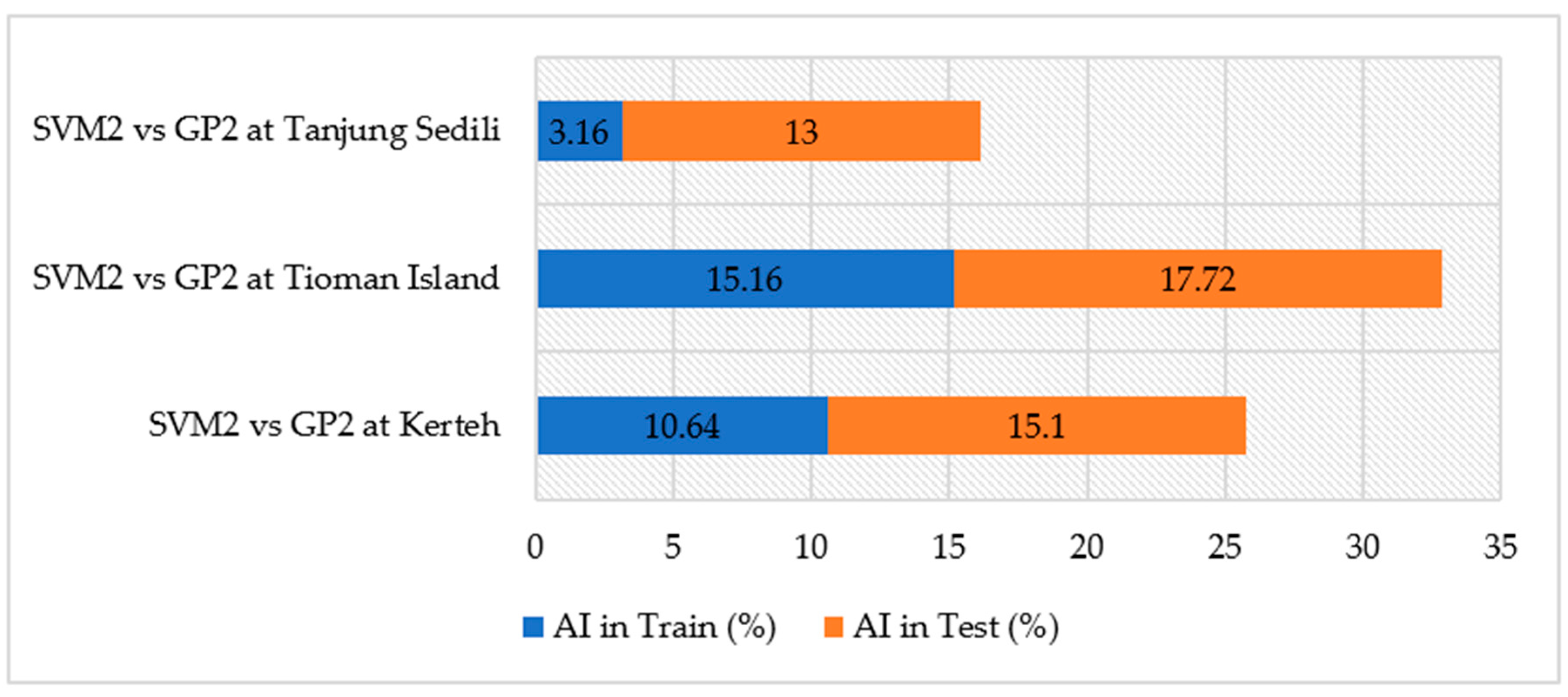
3.6. Comparison of the Accuracy Improvement (AI) in SVM2 and GP2 at the Study Locations

Figure 10 represents the accuracy improvement percentages of SVM2 and GP2 at Kerteh with values of 10.64% and 15.1% during the training and testing stages, respectively. Similar results were obtained at the Tioman Island, denoting that the AI during the training and testing periods did not show a drastic decrease. Hence, both the algorithms with input designs of SVM2 and GP2 were consistent and steady. Furthermore, no sudden substantial drop or rise in percentage can be observed because an increase in accuracy improvement that is within only 5% could be observed during the testing stage. This model input design is suitable for the long-term prediction of SL toward the end of this study because the correlation coefficients for both the models are capable of reaching ideal values with values of 0.75 and above in SVM2 and 0.73 and above in the GP2 model during training and testing, respectively.
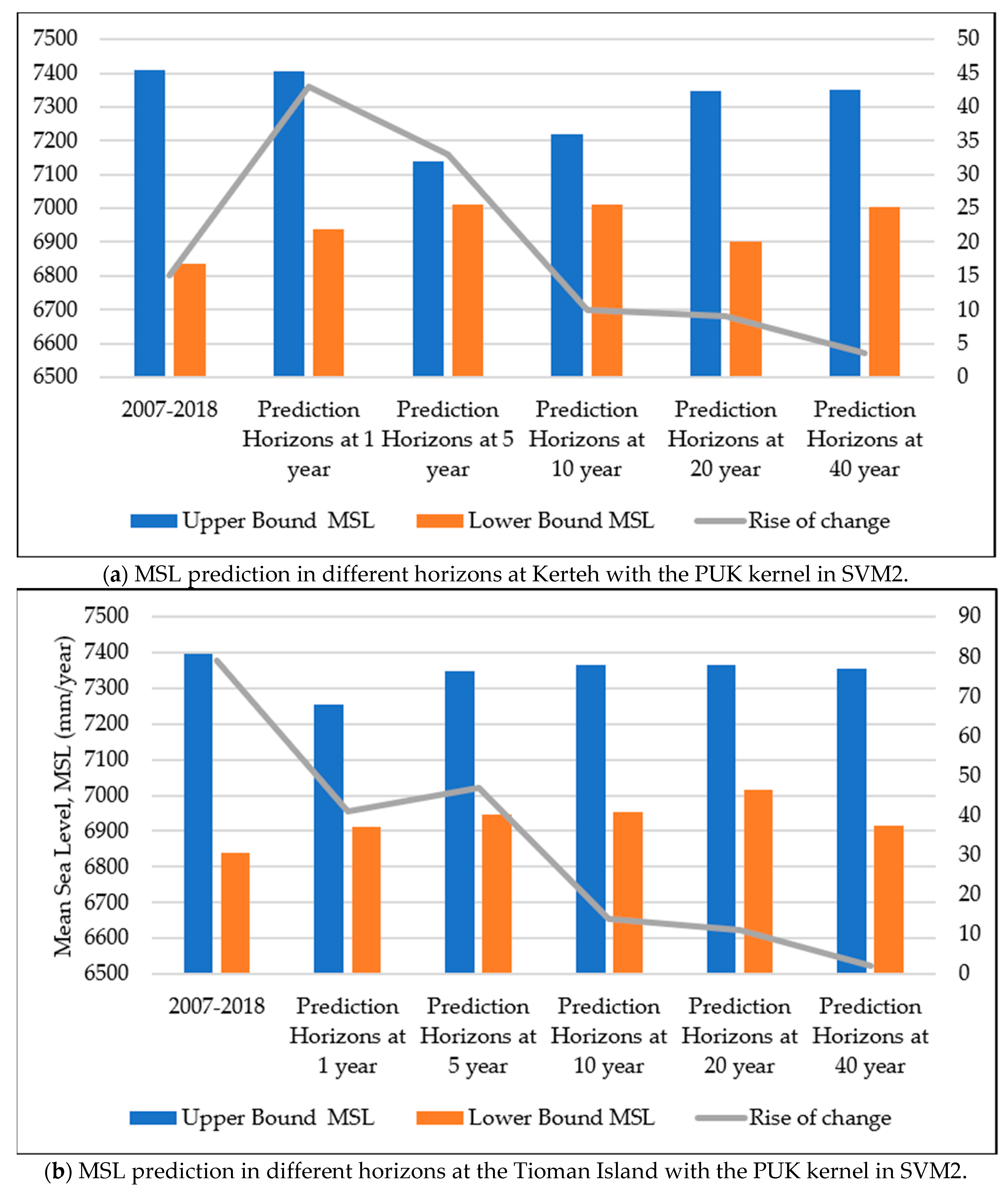
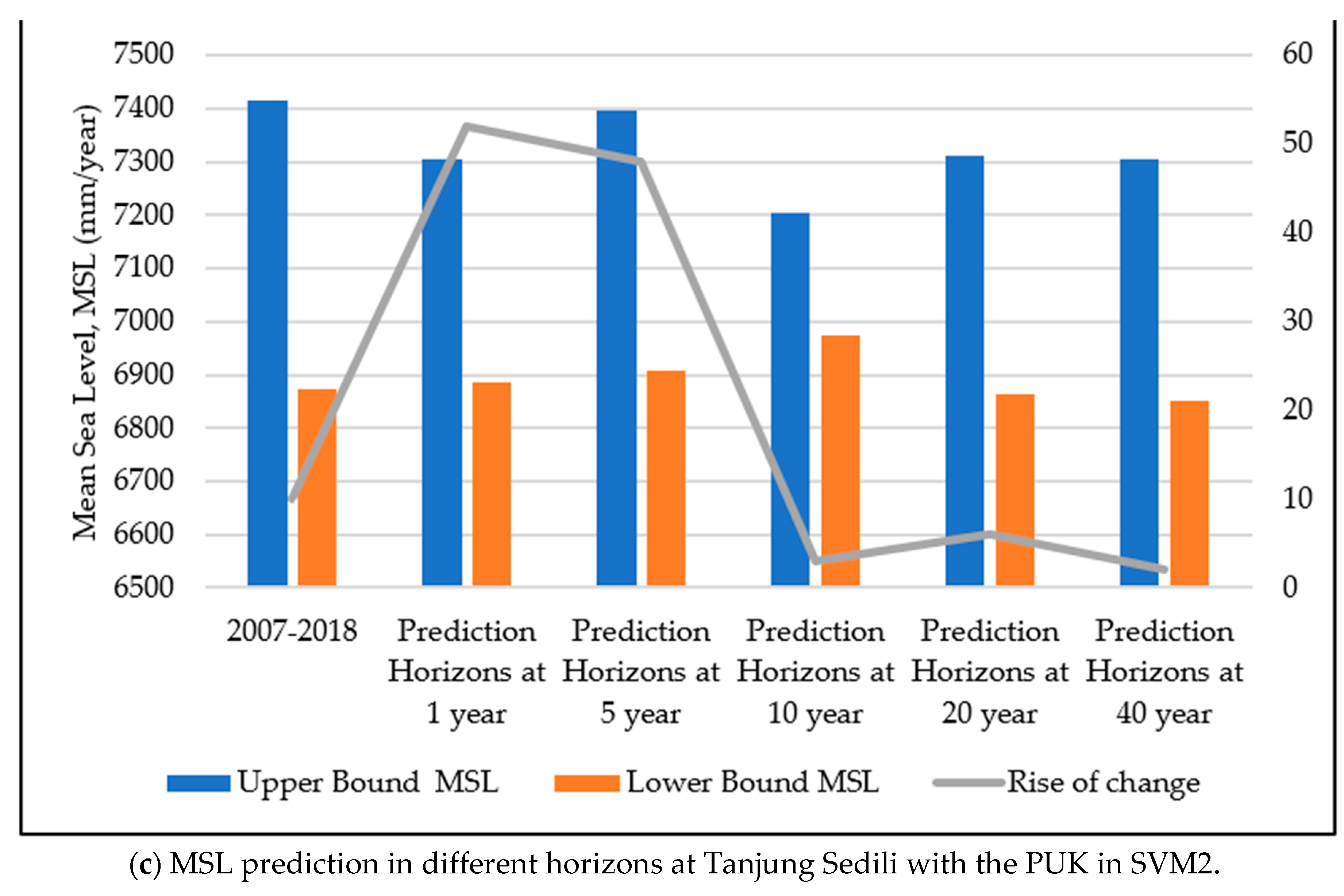
In accordance with Figure 11, the predicted MSL from five different prediction horizons with an SVM2 input design at the study locations are presented with the upper and lower bounds of the predicted MSL. Figure 11 depicts that the highest predicted MSL in the upper bound could be observed at a prediction horizon of 5 years at Tanjung Sedili with a value of 7396 mm. The second highest predicted MSL in the upper bound occurred at prediction horizons of 10 and 20 years at the Tioman Island with a value of 7396 mm. The lowest value in the upper bound of the predicted MSL was observed at Kerteh as 7350 mm at a predicted horizon of 40 years. However, the lowest value of the predicted MSL in the lower bound for all the study locations was between 6836 and 6852 mm. The minimum increase in the predicted MSL was 2.0 mm/year, whereas the maximum increase was 79.0 mm/year.
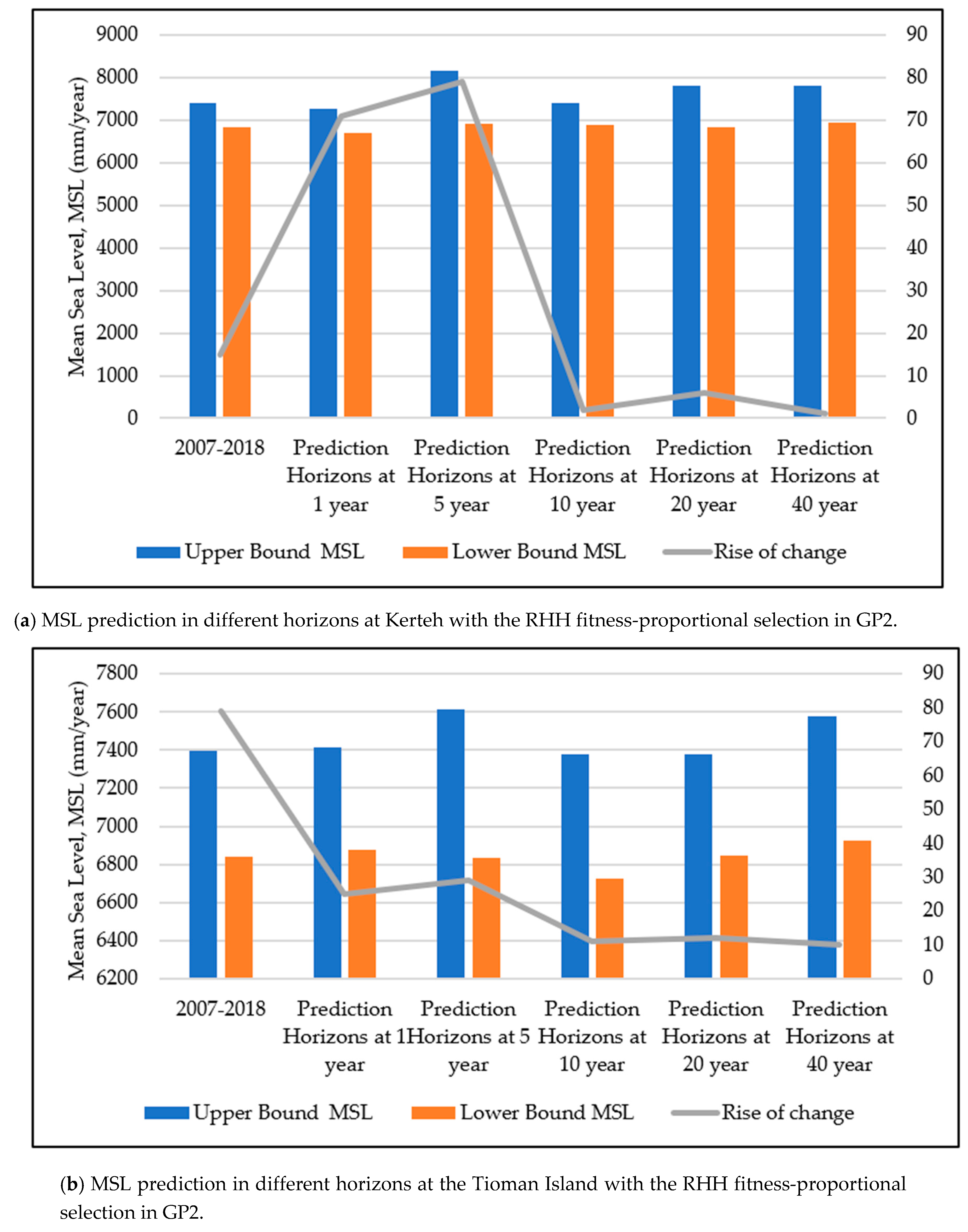
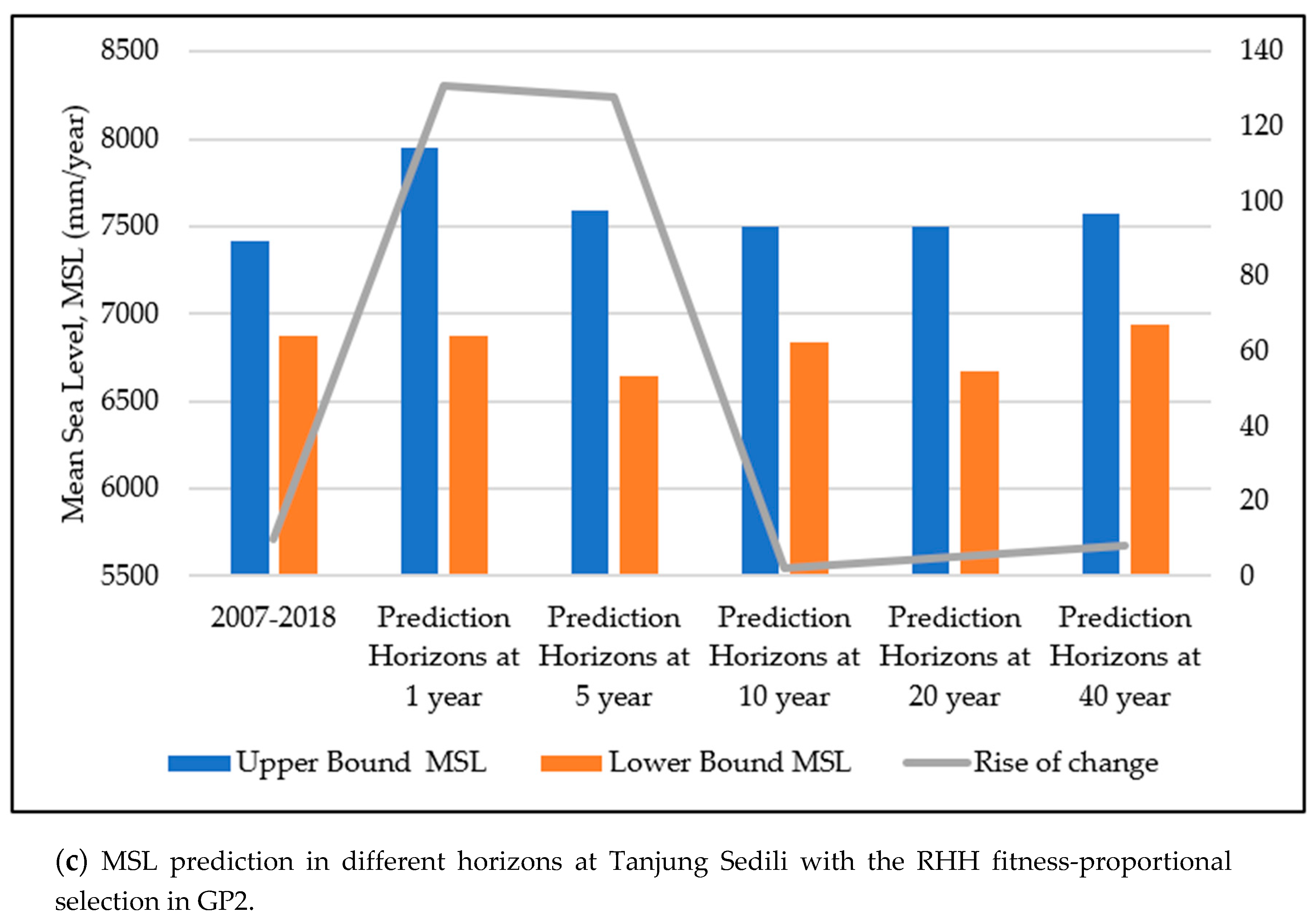
As illustrated in Figure 12, the predicted MSL in five different prediction horizons with GP2 at the study locations are presented with the upper and lower bounds of the predicted MSL. Figure 12 shows that the highest predicted MSL in the upper bound occurred at a prediction horizon of 1 year at Tanjung Sedili and was 7950 mm. The second highest predicted upper bound of the MSL occurred at a prediction horizon of 40 years at Kerteh and was 7805 mm. The lowest value in the upper bound of the predicted MSL was found at a prediction horizon of 5 years at the Tioman Island and was 7616 mm. However, the lowest value of the predicted MSL in the lower bound for all the study locations was between 6835 mm and 6840 mm. The minimum increase in the predicted MSL was 2.0 mm/year, whereas the maximum increase in the predicted MSL was 131.0 mm/year.

4. Conclusions

The capabilities of the SVM and GP models for MMSL prediction were examined herein based on the tide gauge data obtained from 2007 to 2017. SVM methods were compared with their functions, including the NP, RBF, and PUK kernels, to optimize the SVM model. The GP functions, namely RHH with rank selection and fitness-proportional selection, were also compared to assess the prediction accuracy of the GP model. The results indicated that the PUK in SVM2 and RHH with the fitness-proportional selection of the GP2 methods constitutes suitable techniques for analyzing the MMSL prediction and exhibited an effectively higher performance when compared with that exhibited by the remaining SVM and GP techniques. Different prediction horizons (i.e., 1, 5, 10, 20, and 40 years) were developed using SVM and GP to predict the MMSL. The overall results of the MMSL for SVM2 and GP2 at prediction horizons of 1 and 5 years showed an average maximum increment of 75 mm/year, whereas a prediction horizon of 10 years or more showed a decreasing sea level with a minimum average sea level of 10 mm/year at Kerteh, Tioman Island, and Tanjung Sedili. The outcome of MMSL at different prediction horizons implied that both the SVM2 and GP2 models exhibited stable performances. Therefore, both the proposed models are appropriate for predicting MMSL without bias or eliminating the hidden information in the time series. The results obtained from this study provide reliable prediction values with respect to the future increase in sea level at the identified coastal areas. Therefore, effective and economic planning pertaining to the safety and economics of the communities living along the coastal areas of Malaysia can be conducted by various state and federal authorities. Furthermore, the observations of this study could be a promising base for conducting further investigation on the proficiency of the SVM and GP models for sea level prediction in different time horizons. However, this study also exhibits limitations such as data availability. Therefore, conducting future research to perform further analysis on the sensitivity between each input variable with the associated output and identify the weight matrix could be a potential future research direction. Future studies may also focus on improving the proposed model by introducing other complex parameters as the model input, which has not been investigated in this study because of the limitation of the available data.
The modeling implementation process required a relatively long time to achieve the performance objective during training even though the proposed SVM and GP models showed an outstanding performance in case of MMSL prediction. In addition, the maximum relative error was still slightly high. Therefore, integrating the proposed methods (SVM and GP) with an advanced nature-inspired optimization algorithm that could accelerate the searching process for the global optimal solution is recommended to accelerate the training process. Furthermore, a model with an effective preprocessing method that could detect the inherent pattern of the raw data before feed, regardless of being an SVM or GP model, must be adapted to improve the overall prediction accuracy and reduce the maximum error.

Author Contributions

Formal analysis, A.E.-S. (Amr El-Shafie); Methodology, A.N.A.; Resources, A.E.-S. (Ahmed El-Shafie); Supervision, M.A.M. and A.E.-S. (Ahmed El-Shafie); Validation, R.K.I.; Writing-original draft, V.L.; Writing-review & editing, H.A.A.

Funding

Universiti Tenaga Nasional: RJO10436494.

Acknowledgments

The authors gratefully acknowledge the financial support received from Bold 2025 grant coded RJO: 10436494 by Innovation & Research Management Center (iRMC), Universiti Tenaga Nasional (UNITEN) in Malaysia. In addition, the authors would like to thank the Malaysian Meteorological Department (MetMalaysia) for providing data for this research. The authors also would like to thank the strong administration support rendered by the MDPI editorial team especially Assistant Editor, Kate Yang.

Conflicts of Interest

The authors declare no conflicts of interest.

References

  1. Overeem, I.; Syvitski, J.P.M. Dynamics and Vulnerability of Delta Systems; LOICZ Reports & Studies No. 35; GKSS Research Center: Geesthacht, Germany, 2009; p. 54. [Google Scholar]
  2. Atkinson, A.L.; Baldock, T.E.; Birrien, F.; Callaghan, D.P.; Nielsen, P.; Beuzen, T.; Turner, I.I.; Blenkinsopp, C.E.; Ranasinghe, R. Laboratory investigation of the Bruun Rule and beach response to sea level rise. Coast. Eng. 2018, 136, 183–202. [Google Scholar] [CrossRef]
  3. Handoko, E.Y.; Fernandes, M.J.; Lázaro, C. Assessment of altimetric range and geophysical corrections and mean sea surface models-Impacts on sea level variability around the Indonesian seas. Remote Sens. 2017, 9, 102. [Google Scholar] [CrossRef]
  4. Kim, Y.; Newman, G. Climate change preparedness: Comparing future urban growth and flood risk in Amsterdam and Houston. Sustainability 2019, 11, 1048. [Google Scholar] [CrossRef] [PubMed]
  5. Meyssignac, B.; Cazenave, A. Sea level: A review of present-day and recent-past changes and variability. J. Geodyn. 2012, 58, 96–109. [Google Scholar] [CrossRef]
  6. Cazenave, A.; Cozannet, G.L. Sea level rise and its coastal impacts. Earth’s Future 2014, 2, 15–34. [Google Scholar] [CrossRef]
  7. Jackson, L.; Jevrejeva, S. A probabilistic approach to 21st century regional sea level predictions using RCP and High-end scenarios. Glob. Planet. Chang. 2016, 146, 179–189. [Google Scholar] [CrossRef]
  8. Makarynskyy, O.; Makarynska, D.; Kuhn, M.; Featherstone, W.E. Predicting sea level variations with artificial neural networks at Hillarys Boat Harbour, Western Australia. Estuar. Coast. Shelf Sci. 2004, 61, 351–360. [Google Scholar] [CrossRef] [Green Version]
  9. Nicholls, R.J.; Marinova, N.; Lowe, J.A.; Brown, S.; Vellinga, P.; De Gusmão, D.; Hinkel, J.; Tol, R.S.J. Sea-level rise and its possible impacts given a “beyond 4 °C world” in the twenty-first century. Philos. Trans. R. Soc. A Math. Phys. Eng. Sci. 2011, 369, 161–181. [Google Scholar] [CrossRef]
  10. Günaydın, K. The estimation of monthly mean significant wave heights by using artificial neural network and regression methods. Ocean Eng. 2008, 35, 1406–1415. [Google Scholar] [CrossRef]
  11. Ebrahimi, H.; Rajaee, T. Simulation of groundwater level variations using wavelet combined with neural network, linear regression and support vector machine. Glob. Planet. Chang. 2017, 148, 181–191. [Google Scholar] [CrossRef]
  12. Li, D.C.; Han, M.; Wang, J. Chaotic time series prediction based on a novel robust echo state network. IEEE Trans. Neural Netw. Learn. Syst. 2012, 23, 787–799. [Google Scholar] [CrossRef] [PubMed]
  13. Zhao, P.; Xing, L.; Yu, J. Chaotic time series prediction: From one to another. Phys. Lett. A 2009, 373, 2174–2177. [Google Scholar] [CrossRef]
  14. Chau, K.W.; Wu, C.L.; Li, Y.S. Comparison of several flood forecasting models in Yangtze River. J. Hydrol. Eng. 2005, 10, 485–491. [Google Scholar] [CrossRef]
  15. Taormina, R.; Chau, K.W.; Sivakumar, B. Neural network river forecasting through baseflow separation and binary-coded swarm optimization. J. Hydrol. 2015, 529, 1788–1797. [Google Scholar] [CrossRef]
  16. Pashova, L.; Popova, S. Daily sea level forecast at tide gauge Burgas, Bulgaria using artificial neural networks. J. Sea Res. 2011, 66, 154–161. [Google Scholar] [CrossRef]
  17. Li, M.; Li, Y.; Leng, J. Power-type functions of prediction error of sea level time series. Entropy 2015, 17, 4809–4837. [Google Scholar] [CrossRef]
  18. Beale, M.H.; Hagan, M.T.; Demuth, H.B. Neural Network Toolbox 7 User’s Guide; The MathWorks Inc.: Natick, MA, USA, 2010; p. 951. [Google Scholar]
  19. Chang, H.-K.; Lin, L.-C.H. Multi-point tidal prediction using artificial neural network with tide-generating forces. Coast. Eng. 2006, 53, 857–864. [Google Scholar] [CrossRef]
  20. Demuth, H.B.; Beale, M.H.; Hagan, M.T. Mathworks. Neural Network Toolbox User’s Guide; The MathWorks Inc.: Hong Kong, China, 2008. [Google Scholar]
  21. Vapnik, V.N. Statistical Learning Theory; Wiley: New York, NY, USA, 1998; p. 768. [Google Scholar]
  22. Wang, D.; Peng, J.; Yu, Q.; Chen, Y.; Yu, H. Support vector machine algorithm for automatically identifying depositional microfacies using well logs. Sustainability 2019, 11, 1919. [Google Scholar] [CrossRef]
  23. Asefa, T.; Kemblowski, M.; McKee, M.; Khalil, A. Multi-time scale stream flow predictions: The support vector machines approach. J. Hydrol. 2006, 318, 7–16. [Google Scholar] [CrossRef]
  24. Lu, M.; Zhang, Z.Y. Application of support vector machine in runoff forecast. China Rural. Water Hydropower 2006, 2, 47–49. [Google Scholar]
  25. Pochwat, K.B.; Słyś, D. Application of artificial neural networks in the dimensioning of retention reservoirs. Ecol. Chem. Eng. 2018, 25, 605–617. [Google Scholar] [CrossRef]
  26. Genetic Programming. Available online: http://geneticprogramming.com/ (accessed on 30 June 2019).
  27. Sipper, M.; Olson, R.S.; Moore, J.H. Evolutionary computation: The next major transition of artificial intelligence? BioData Mining. 2017, 26, 10. [Google Scholar] [CrossRef] [PubMed]
  28. Koza, J.R. Genetic Programming: On the Programming of Computers by Means of Natural Selection; MIT Press: Cambridge, MA, USA, 1992. [Google Scholar]
  29. Floudas, C.; Parlalos, P. Collection of Test Problems for Constrained Global Optimization Algorithms; Springer: Berlin, Germany, 1990; Volume 455. [Google Scholar]
  30. Floudas, C.; Pardolos, M. Encyclopedia of Optimization, 2nd ed.; Springer: Berlin, Germany, 2009. [Google Scholar]
  31. Ali Ghorbani, M.; Khatibi, R.; Aytek, A.; Makarynskyy, O.; Shiri, J. Sea water level forecasting using genetic programming and comparing the performance with Artificial Neural Networks. Comput. Geosci. 2010, 36, 620–627. [Google Scholar] [CrossRef]
  32. Yan, J.; Zongbao, X.; Yongchuan, Y.; Hongxia, X.; Kaili, G. Application of a hybrid optimized BP network model to estimate water quality parameters of Beihai Lake in Beijing. Appl. Sci. 2019, 9, 1863. [Google Scholar] [CrossRef]
  33. Barge, J.; Hatim, S. An ensemble empirical mode decomposition, self-organizing map, and linear genetic programming approach for forecasting river streamflow. Water 2016, 8, 247. [Google Scholar] [CrossRef]
  34. Macek, K. The pareto principle in datamining: An above-average fencing algorithm. Acta Polytech. 2008, 55–59. [Google Scholar]
  35. Lai, V.; Najah, A.; Malek, M.A.; El-Shafie, A. Evolutionary algorithm for forecasting mean sea level based on meta-heuristic approach. Int. J. Civil Eng.Technol. 2018, 9, 1404–1413. [Google Scholar]
  36. Olivia Muslim, T.; Najah, A.; Malek, M.A.; El-Shafie, A. Investigating the impact of wind on sea level rise using multilayer perceptron neural network (MLP-NN) at coastal area, Sabah. Int. J. Civil Eng. Technol. 2018, 9, 646–656. [Google Scholar]
  37. Imani, M.; Kao, H.-C.; Lan, W.-H.; Kuo, C.-Y. Daily sea level prediction at Chiayi coast, Taiwan using extreme learning machine and relevance vector machine. Glob. Planet. Chang. 2018, 161, 211–221. [Google Scholar] [CrossRef]
  38. El-Shafie, A.; Najah, A.; Lai, V. An application of artificial intelligence (AI) technique for wave prediction in Terengganu. J. Energy Environ. 2016, 8, 34–40. [Google Scholar]
  39. Holgate, S.J.; Matthews, A.; Woodworth, P.L.; Rickards, L.J.; Tamisiea, M.E.; Bradshaw, E.; Foden, P.R.; Gordon, K.M.; Jevrejeva, S.; Pugh, J. New Data Systems and Products at the Permanent Service for Mean Sea Level. J. Coast. Res. 2013, 29, 493–504. [Google Scholar]
  40. Varikoden, H.; Samah, A.; Babu, C. Spatial and temporal characteristics of rain intensity in the peninsular Malaysia using TRMM rain rate. J. Hydrol. 2010, 387, 312–319. [Google Scholar] [CrossRef] [Green Version]
  41. Reynolds, R.; Smith, T.; Liu, C.; Chelton, D.; Casey, K.; Schlax, M. Daily high-resolution blended analyses for sea surface temperature. J. Clim. 2007, 20, 5473–5496. [Google Scholar] [CrossRef]
  42. Cherkassky, V.; Xuhui, S.; Mulier, F.M.; Vapnik, V.N. Model complexity control for regression using VC generalization bounds. IEEE Trans. Neural Netw. 1999, 10, 1075–1089. [Google Scholar] [CrossRef] [PubMed]
  43. Hastie, T.; Tibshirani, R.; Friedman, J. The Elements of Statistical Learning; Data Mining, Inference and Prediction; Springer: New York, NY, USA, 2001. [Google Scholar]
  44. Kwok, J.T. Linear dependency between ε and the input noise in ε –support vector regression. In International Conference on Artificial Neural Networks; Dorffner, G., Bishof, H., Hornik, K., Eds.; Springer: Berlin/Heidelberg, Germany, 2001; pp. 405–410. [Google Scholar]
  45. Hipni, A.; El-shafie, A.; Najah, A.; Karim, O.A.; Hussain, A.; Mukhlisin, M. Daily forecasting of dam water levels: Comparing a support vector machine (SVM) model with adaptive neuro fuzzy inference system (ANFIS). Water Resour. Manag. 2013, 27, 3803–3823. [Google Scholar] [CrossRef]
  46. Najah, A.A.; El-Shafie, A.; Karim, O.A.; Jaafar, O. Water quality prediction model utilizing integrated wavelet-ANFIS model with cross validation. Neural Comput. Appl. 2010, 21, 833–841. [Google Scholar] [CrossRef]
  47. El-Shafie, A.H.; El-Shafie, A.; El Mazoghi, H.G.; Shehata, A.; Taha, M.R. Artificial neural network technique for rainfall forecasting applied to Alexandria, Egypt. Int. J. Phys. Sci. 2010, 6, 1306–1316. [Google Scholar]
  48. Mitchell, T. Machine Learning; McGraw Hill: New York, NY, USA, 2017. [Google Scholar]
  49. Banzhaf, W. Genetic Programming; Springer: Berlin/Heidelberg, Germany, 1998. [Google Scholar]
  50. Madsen, P.; Hegelund, T. On-gradient subroutines for non-linear optimization, Report NI-95- 05, Numerisk Institut, Technical U. DenmarkSMITH, S. F. A Learning System Based on Genetic Adaptive Algorithms. Ph.D. Thesis, University of Pittsburgh, Pittsburgh, PA, USA, 1980. [Google Scholar]
  51. Luke, S.; Panait, L. Fighting bloat with nonparametric parsimony pressure. In Proceedings of the Parallel Problem Solving from Nature; Springer: Berlin/Heidelberg, Germany, 2002; pp. 411–421. [Google Scholar]
  52. Luu, Q.H.; Tkalich, P.; Tay, T.W. Sea level trend and variability around Peninsular Malaysia. Ocean Sci. 2015, 11, 617–628. [Google Scholar] [CrossRef] [Green Version]
  53. Luke, S.; Panait, L. Lexicographic parsimony pressure. In Proceedings of the Genetic and Evolutionary Computation Conference, New York, NY, USA, 9–13 July 2002; Morgan Kaufmann Publishers Inc.: Burlington, MA, USA, 2002; pp. 829–836. [Google Scholar]
  54. Kashid, S.; Rajib, M. Prediction of monthly rainfall on homogeneous monsoon regions of India based on large scale circulation patterns using genetic programming. J. Hydrol. 2012, 454–455, 26–41. [Google Scholar] [CrossRef]
  55. Langdon, W.; Poli, R. Foundations of Genetic Programming; Springer: Berlin, Germany, 2002. [Google Scholar]
Figure 1. Study locations in the east coast of Peninsular Malaysia.
Sustainability 11 04643 g001
Figure 2. The architecture of the support vector machine.
Sustainability 11 04643 g002
Figure 3. Typical tree structure for ( x 1 x 2 + x 3 ) 2.
Sustainability 11 04643 g003
Figure 4. Flow chart of the prediction methodology of historical monthly mean sea level (MMSL) using the support vector machine (SVM) and genetic programming (GP) algorithms.
Sustainability 11 04643 g004
Figure 5. Scatter plot of the actual and predicted monthly mean sea levels obtained from the PUK of SVM modeling during the training and testing periods at (a) Kerteh, (b) the Tioman Island, and (c) Tanjung Sedili.
Sustainability 11 04643 g005aSustainability 11 04643 g005b
Figure 6. Model performances of the PUK in the SVM model at (a) Kerteh, (b) the Tioman Island, and (c) Tanjung Sedili.
Sustainability 11 04643 g006
Figure 7. Scatter plots of the actual and predicted monthly mean sea levels obtained from ramped half–half (RHH) and the fitness-proportional selection of the GP model during the training and testing periods at (a) Kerteh, (b) the Tioman Island, and (c) Tanjung Sedili.
Sustainability 11 04643 g007aSustainability 11 04643 g007b
Figure 8. Model performances of GP2 with RHH and the fitness-proportional selection model at (a) Kerteh, (b) the Tioman Island, and (c) Tanjung Sedili.
Sustainability 11 04643 g008
Figure 9. Comparison of the average error percentages in case of SVM2 and GP2 at the study locations.
Sustainability 11 04643 g009
Figure 10. Summary of the accuracy improvement of SVM and GP at the study locations.
Sustainability 11 04643 g010
Figure 11. MSL prediction at different prediction horizons with the PUK in SVM2: (a) Kerteh, (b) Tioman Island, and (c) Tanjung Sedili.
Sustainability 11 04643 g011aSustainability 11 04643 g011b
Figure 12. MSL prediction at different prediction horizons with the RHH fitness-proportional selection in GP2: (a) Kerteh, (b) the Tioman Island, and (c) Tanjung Sedili.
Sustainability 11 04643 g012aSustainability 11 04643 g012b
Table 1. Arrangement of the statistical data obtained from the study locations between January 1, 2007 and December 31, 2017.
Statistics/Study LocationKertehTioman IslandTanjung Sedili
Rainfall Amount (mm)Mean Cloud Cover (Okta)Mean Sea Level (mm)SST (°C)Rainfall Amount (mm)Mean Cloud Cover (Okta)Mean Sea Level (mm)SST (°C)Rainfall Amount (mm)Mean Cloud Cover (Okta)Mean Sea Level (mm)SST (°C)
Maximum1645.207.407411.0031.00880.407.40739831.0574.207.40741531.0
Minimum2.006.386836.0026.402.006.60683926.910.006.60687227.0
Sum73,322.472770.402,806,123.0011,494.2727,816.70923.49935,8433,835.2012,798.98923.55934,6353844.93
Average185.167.007086.1729.03210.736.997,089.729.0596.967.007080.5729.13
Mean Standard deviation192.230.109132.800.89162.800.08129.160.85119.800.09133.550.79
Table 2. Major influencer of variables for three different kernels in the SVM.
Type of Kernel FunctionsTuning or Affecting Parameters
Normalized polynomial kernel (NP)d(exponent), C, and ϵ
Radial basis kernel (RBF)ɣ, C, and ϵ
Pearson universal kernel (PUK)ω, σ, C, and ϵ
Table 3. Summary of the SVM model performance with different kernel types and input designs at Kerteh.
Input Design SVM1SVM2SVM3
Kernel Type/ Model PerformanceNPRBFPUKNPRBFPUKNPRBFPUK
TrainTestTrainTestTrainTestTrainTestTrainTestTrainTestTrainTestTrainTestTrainTest
R0.34100.5100.4430.5230.2280.7510.7240.6350.6470.8630.8610.7780.6970.5120.4620.7660.708
RMSE (mm)144.00140.40124.79140.16117.63157.1286.8974.81118.24134.4069.1783.06110.6103.14124.63139.4188.65106.15
SI1.201.171.031.160.981.30.720.620.981.120.570.690.920.851.031.160.730.88
MAE (mm)112.72133.14124.79140.16117.63157.1295.198.795.399.946.568.184.988.099.8102.462.383.9
MAPE (%)68.285.148.952.346.776.132.235.345.746.925.625.236.843.749.951.837.541.7
Table 4. Cross-validation of the Pearson universal kernel (PUK) at the study locations.
Study LocationsKertehTioman IslandTanjung SediliCross-ValidationNo. of Support VectorCapacity
Model PerformancesTrainTestTrainTestTrainTest
R0.7710.7570.7720.7960.6990.786101181.0
R0.7770.7660.7790.8050.7060.79591181.0
R0.7710.7570.7720.7960.6990.78681181.0
R0.7640.7490.7650.7870.6920.77771181.0
R0.7570.7400.7580.7780.6850.76861181.0
R0.7500.7310.7510.7690.6780.75951181.0
R0.7430.7220.7450.7605000.6720.75041181.0
R0.7370.7130.7380.7510.6650.74131181.0
R0.7300.7040.7310.7420.6580.73221181.0
Table 5. Summary of the GP model performances with different kernel types and input designs at Kerteh.
Input DesignGP1GP2GP3
Selections/Model PerformanceRHH and Fitness Proportionate SelectionRHH and Rank SelectionRHH and Fitness Proportionate SelectionRHH and Rank SelectionRHH and Fitness Proportionate SelectionRHH and Rank Selection
TrainTestTrainTestTrainTestTrainTestTrainTestTrainTest
R0.7690.5710.6820.2150.780.7480.780.450.7560.570.730.40
RMSE (mm)88.62117.1687.39185.6886.6989.288.63120.3290.94124.4186.58120.27
SI1.20.670.750.3251.31.021.30.521.080.670.930.49
MAE (mm)125.6135.9120.3159.7103.2106.5121.3144.7115.5138.2128.9140.2
MAPE (%)35.943.538.285.222.925.023.059.729.249.633.653.7
Table 6. Crossover processing for the RHH and fitness-proportional selection at the study locations.
Study LocationsKertehTioman IslandTanjung SediliCrossoverGeneration
Model PerformancesTrainTestTrainTestTrainTest
R; Last Change0.758;3750.452;3750.689;1920.578;1920.735;3710.73;3710.2300
R; Last Change0.708;3770.55;3770.697;3940.524;3940.719;2700.487;2700.4300
R; Last Change0.762;3690.748;3690.702;2650.591;2650.722;870.776;870.6300
R; Last Change0.682;3410.498;3410.722;3450.718;3450.71;2510.703;2510.8300

