Artificial Intelligence Techniques in Power Systems, pp 220 237 K. Warwick, A.O. Ekwue and R. Aggarwal,1997, IEE
|
Chapter 10 Scheduling Maintenance of Electrical Power Transmission Networks Using Genetic Programming W. B. Langdon , P. C. Treleaven University College London |
Abstract
The National Grid Company Plc. is responsible for the maintenance of the high voltage electricity transmission network in England and Wales. It must plan maintenance so as to minimise costs taking into account:
i.e. that part not undergoing maintenance.
Previous work showed the combination of a Genetic Algorithm using an order or permutation chromosome combined with hand coded ‘Greedy’ Optimisers can readily produce an optimal schedule for a four node test problem [10]. Following this the same GA has been used to find low cost schedules for the South Wales region of the UK high voltage power network.
This paper describes the evolution of the best known schedule for the base South Wales problem using Genetic Programming starting from the hand coded heuristics used with the GA.
1 Introduction
In England and Wales electrical power is transmitted by a high voltage electricity transmission network which is highly interconnected and carries large power flows. It is owned and operated by The National Grid Company plc. (NGC) who maintain it and wish to ensure its maintenance is performed at least cost, consistent with plant safety and security of supply.
There are many components in the cost of planned maintenance. The largest is the cost of replacement electricity generation, which occurs when maintenance of the network prevents a cheap generator from running so requiring a more expensive generator to be run in its place.
The task of planning maintenance is a complex constrained optimization scheduling problem. The schedule is constrained to ensure that all plant remains within its capacity and the cost of replacement generation, throughout the duration of the plan is minimised. At present maintenance schedules are produced manually by NGC's Planning Engineers (who use computerised viability checks on the schedule after it has been produced).
Previous work showed the combination of a Genetic Algorithm (GA) [7], using an order or permutation chromosome combined with hand coded ‘Greedy’ Optimises can readily produce an optimal schedule for a four node test problem [10] (see also Figure 5). Following this the same GA has been used to find low cost year long maintenance schedules for the South Wales region of the UK high voltage power network. [5] used a linear chromosome with non-binary alleles [13] to solve the four node problem but was less successful on the larger South Wales problem).
This paper describes the evolution of better ‘greedy’ optimizers for the South Wales problem using genetic programming (GP) starting from the hand coded heuristic used with the GA. Section 2 describes the South Wales region of the UK high voltage power transmission network. The fitness function used to cost maintenance schedules and scheduling heuristics are the same as used in the earlier GA approaches (Sections 3, 4 and 5 are based on [10]). Section 6 describes in detail the genetic programming experiment and the results obtained while Section 7 describes other approaches that might be tried and possible further work.
2 South Wales Region of UK Electricity Network
The South Wales region of the UK electricity network carries power at 275K Volts and 400K Volts between electricity generators and regional electricity distribution companies and major industrial consumers. The region covers the major cites of Swansea, Cardiff, Newport and Bristol, steel works and the surrounding towns and rural areas (see Figure 1). The mayor sources of electricity are in feeds (2) from the English Midlands, coal fired generation at Aberthaw, nuclear generation at Oldbury and oil fired generation at Pembroke. Both demand for electricity and generation change significantly through the year (See Figures 2 and 3).
Figure 1 South Wales Region High Voltage Network
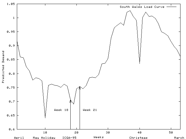
Figure 2 Predicted Demand in South Wales Region
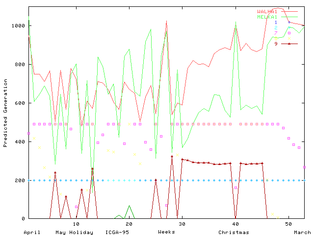
Figure 3 Predicted Generation in South Wales Region
The representation of the electricity network used in these experiments is firmly based upon the engineering data available for the physical network however a number of simplifications have to be made. Firstly the regional network has been treated as an isolated network, its connections to the rest of the network have been modelled by two sources of generation connected by a pair of low impedance high capacity conductors. Secondly the physical network contains short spurs run to localised load points such as steel works. These ‘T’ points have been simplified (e.g. by inserting nodes into the simulation) so all conductors connect two nodes. The industry standard DC load flow approximation is used to calculate power flows through the network.
In the experiments reported in this paper the maintenance planning problem for the South Wales region has been made deliberately more difficult than the true requirement. In these experiments:
The requirement that the network should be fault resistant during maintenance is not considered in this paper. This is because consideration of potential network faults is highly CPU intensive. The permutation GA approach has been taken further than the GP approach and acceptable schedules have been evolved which do consider network robustness.
3 Approximating Replacement Generation Costs
NGC use computer tools for costing maintenance schedules, however because of their computational complexity, it was felt that these were unsuitable for providing the fitness function. Instead our fitness function is partially based upon estimating the replacement generation costs that would occur if a given maintenance plan were to be used. The estimate is made by calculating the electrical power flows assuming the maintenance will not force a change in generation. In practice alternative generators must be run to reduce the power flow through over loaded lines in the network. The cost of the alternative generators is modelled by setting the amount of replacement generation equal to the excess power flow and assuming alternative generators will be a fixed amount more expensive than the generators they replace.
4 The Fitness Function
The GA's fitness function is composed of two parts; a benefit for performing maintenance plus penalties for exceeding line ratings, isolating nodes and splitting the network.
4.1 Maintenance Benefits
The maintenance requirements of the different components of the transmission network vary both in terms of the number of weeks required to perform them and their urgency. It may be advisable to hold over less urgent maintenance until the following year. However maintenance requirements have been both simplified and made more onerous by requiring all lines to be maintained exactly once, assuming each will take four weeks and giving them all the same benefit.
Should a trial maintenance plan schedule a line for maintenance, its fitness is improved by the maintenance benefit. There is no additional benefit or penalty from additional maintenance. The total benefit is obtained by summing across all lines for the whole year.
4.2 Over Loading Costs
In order to calculate the line overloading costs, we must first determine which generators are to be used and when. This is done by using the available generators in strict price order (cheapest first) until the predicted demand for each week is met (see Figures 2 and 3). This is known as the merit order dispatch. It is fixed and therefore the same for all trial schedules.
For each week of a trial schedule the predicted demand and the merit order dispatch are used in a ‘DC load flow’ analysis which calculates the power flow through every line in the network. The over loading cost for each line is proportional to the amount the power flow though it exceeds its normal operating limit (it is zero if within the limit). The total over loading costs are the sum over each week of the maintenance plan and over all lines in the network.
4.3 Avoiding Isolating Nodes or Splitting the Network
From an operational point of view, no acceptable maintenance schedule would ever isolate a generation or demand node from the rest of the network or split the network. However the GA fitness function must be able to cope with every schedule that is generated. The ‘DC load flow’ algorithm cannot cope with either as they require it to invert a singular matrix. Therefore the fitness function looks for these conditions and defines a fitness for them without calculating power flows.
As both represent highly unfit solutions, weeks of a schedule that cause either contribute a high penalty to the schedule's whole fitness. The penalty for each isolated node is proportional to the load or expected generation at that node. The penalty for a network split is even more severe; it is proportional to the total load across the whole network in that week.
4.4 Combined Fitness Measure
The complete fitness measure is expressed in Megawatt weeks (1 Megawatt (MW) = 1340 horsepower) and is given by the following formula:
![]()
|
|
If network_split Then S1 x total demand Else If isolate_nodes ò
1 Then S2 x Else |
The first summation being over all target maintenance (N.B. the trial plan's cost is increased by Kt if the corresponding maintenance is not scheduled). The second outer summation being over each week of the maintenance plan; the first inner one, being over all isolated nodes, and the second, over all lines in the network.
For the South Wales problem the same values of Kt, S1 and S2 as the four node system where used. i.e. Kt, is 4,000 MW and S1 = S2 = 5. [5] verified the values used for the four node problem are applicable to the South Wales region.
5 Greedy Optimizers
The most successful approach taken so far to solving the power transmission network maintenance scheduling problem has been to split the problem in two; a GA and a ‘greedy optimizer’. The greedy optimizer is presented with a list of work to be done (i.e. lines to be maintained) by the GA It schedules those lines one at a time, in the order presented by the GA, using some problem dependent heuristic. Figure 4 schematic shows this schematically, whilst the dotted line on Figure 5 dotted shows an order in which lines are considered.
Not all figures are online
Figure 4 Hybrid GA and ‘greedy optimizer’
Not all figures are online
Figure 5 Example order (dotted) in which lines are considered by a ‘greedy optimizer’ for the four node problem
This approach of hybridising a GA with a problem specific heuristic has been widely studied. Davis [2] for example firmly advocates using hybrid Gas when attempting to solve difficult real world problems. Hybrid GAs, of various sorts, have been used on a number of scheduling, problems (e.g. flight crew scheduling [12], task scheduling [14] and job-shop and open-shop scheduling [3,4,16].
A variety of heuristics of increasing sophistication and computational complexity have been tried on the four-node problem which yielded progressively better results. The two that are also used in the GP approach are described next.
5.1 Heuristic 2 - Minimum Power Flow
A greedy optimizer was devised which scheduled the maintenance of each line in the week in which the power flow through it is a minimum. In the event of a tie the earlier week is chosen. As each line is scheduled, the power flows through the rest of the network are recalculated.
In the case of the four node network, using this heuristic the GA was able to devise low cost schedules which ensured all the required maintenance was done which did not split the network or shed load. This was achieved by performing maintenance when the demand was least, however it could not produce the optimal schedule.
5.2 Heuristic 4 - Minimum Increase in Line Cost
The other greedy optimizers had been based on the assumption that placing a line in maintenance was bound to increase the power flows on the remaining lines and so must increase line costs (or leave them unchanged). Whilst it is theoretically possible for the change in power flows to decrease line costs it was assumed that this would not occur in practice. The motivation for this greedy scheduler was the realisation that it is possible to schedule some lines so that they reduce line costs. (This is the case of the four node problem and is apparently also true of some real power networks).
The least increase in line cost optimizer schedules maintenance in the week in which maintaining it would lead to the least increase in line costs (or in which there is most decrease). If there is a tie the earliest week is used. N.B. this optimizer looks one week ahead whereas the others make their decisions using only the lines that have already been scheduled.
Using this heuristic the GA easily manages to find the optimal solution to the four node problem. A version modified to take into account maintenance takes four weeks rather than one in the South Wales problem produced an acceptable schedule for South Wales with a cost of 616MW weeks.
6 Genetic Programming Solution
A number of different GP approaches have been tried on these problems. While a ‘pure’ GP approach can find the optimal solution to the four node problem without the need for hand coded heuristics on the South Wales problem, possibly due to insufficient resources, it has not been able to do as well as the best solution produced by the GA and ‘greedy optimizer’ combination. The remainder of this section describes the evolution of lower cost schedules using a GP population which is ‘seeded’ with the two heuristics described in Sections 5.1 and 5.2.
6.1 Architecture
Each individual in the GP population consists of a single tree. This program is called once for each line that is to be maintained, its return value is converted from floating point to an integer which is treated as the first week in which to schedule maintenance of that line. If this is outside the legal range 1...50 then that line is not maintained.
The lines are processed in fixed but arbitrary order given by NGC when the network was constructed. Thus the GP approach concentrates upon evolving the scheduling heuristic whereas in the GA approach this is given and the GA searches for the best order in which to ask the heuristic to process the lines.
6.2 Choice of Primitives
Table 2 shows the functions, terminals and parameters used are given in Table 2 (parameters not given are as [9]). The function and terminal sets include indexed memory, loops and network data.
Indexed memory was deliberately generously sized to avoid restricting the GP's use of it. It consists of 4,001 memory cells each containing a single precision floating point value. They had addresses in the range -2000 ... + 2000. Memory primitives (read, set, swap) had defined behaviour which allows the GP to continue on addressing errors. All stored data within the program is initialised to zero before the trial program is executed for the first line. It is not initialised between runs of the same trial program.
The ‘for’ primitive takes three arguments, an initial value for the loop control variable, the end value and a subtree to be repeatedly executed. It returns the last value of the loop control variable. A run time check prevents loops being nested more than four deep and terminates execution of any loop when more than 10,000 iteration in total have been executed in any one program call. I.e. execution of different loops contribute to the same shared limit. The current value of the innermost for loop control variable is given by the terminal i0, that of the next outer loop by i1, the control variable of the next outer loop by terminal i2 and so on. When not in a loop nested to depth n , in is zero.
The network primitives return information about the network as it was just before the test program was called. Each time a change to the maintenance schedule is made, power flows and other affected data are recalculated before the GP tree is executed again to schedule maintenance of the next line. The network primitives are those available to the C programmer who programmed the GA heuristics and the fitness function (see Table 1). Where these primitives take arguments, they are checked to see if they are within the legal range. If not the primitive normally evaluates to 0.0.
Table 1 Network Primitives
|
Primitive |
Meaning |
|
max |
10.0 |
|
ARG1 |
Index number of current line, 1.0 ... 42.0 |
|
nn |
Number of nodes in network, 28.0 |
|
nl |
Number of lines in network, 42.0 |
|
nw |
Number of weeks in plan, 53.0 |
|
nm_weeks |
Length of maintenance outage, 4.0 |
|
P(n) |
Power injected at node n in 100MW. Negative values indicate demand. |
|
NNLK(l) |
Node connected to first end of line l |
|
NNLJ(l) |
Node connected to end of line l |
|
XL(l) |
Impedance of line l W |
|
LINERATING |
Power carrying capacity of line l in MW |
|
MAINT(w, l) |
1.0 if line l is scheduled for maintenance in week w , otherwise 0.0 |
|
splnod(w, n) |
1.0 if node n is isolated in week w of the maintenance plan, 0.0 otherwise. |
|
FLOW(w, n) |
Power flow in line l from first end to second in week w, negative if flow is reversed MW. |
|
shed(w, l)) |
Demand or generation at isolated nodes in week w if line l is maintained in that week in addition to current scheduled maintenance MW. |
|
loadflow(w, l, a) |
Performs a load flow calculation for week w assuming line l is maintained during the week in addition to the currently scheduled maintenance. Returns cost of schedule for week w. If a is valid also sets memory locations a ... a+nl-1 to the power flows through the network MW |
|
fit(w) |
Returns the current cost of week w of the schedule |
Table 2 South Wales Problem
|
Primitive |
Meaning |
|
Object |
Find a program that yields a good maintenance schedule when presented with maintenance tasks in network order |
|
Architecture |
One result producing branch |
|
Primitives |
ADD, SUB, MUL, DIV, ABS, mod, int, PROG2, IFLTE, Ifeq, Iflt, 0, 1, 2, max, ARG1, read, set, swap, for, i0, i1, i2, i3, i4, nn, nl, nw, nm P, NNLK, NNLJ, XL, LINERATING, MAINT, splnod, FLOW, shed, loadflow fit |
|
Max Prog. Szie |
200 |
|
Fitness Case |
All 42 lines to be maintained |
|
Selection |
Pareto Tournament group size of 4 (with niche sample size 81) used for both parent selection and selecting programs to be removed from the population. Pareto components: Schedule cost, CPU penalty above 100,000 per line, schedule novelty. Steady state panmitic population. Elitism used on schedule cost |
|
Wrapper |
Convert to integer. If ò 1 and ó 50, treat as week to schedule start of maintenance of current line, otherwise the current line is not maintained. |
|
Parameters |
Pop = 1000, G = 50, no aborts. pc = 0.9, psubtree mutation = 0.05, pnode mutation = 0.05. Node mutation rate = 10/1024. |
|
Success Predicate |
Schedule cost ó 616. |
6.3 Mutation
Approximately 90% of new individual are created by crossover between two parents using GP crossover (as [8] except only one individuals is created at a time). The remainder are created by mutating a copy of a single parent. Two forms of mutation are used with equal likelihood. In subtree mutation [8] a single node within the program is chosen at random. This is the root of a sub tree which is removed and replaced with a randomly generated new sub tree. The other form or mutation selects nodes at random (with a frequency of 10/1024) and replaces them with a randomly selected function (or terminal) which takes the same number of arguments. Thus the tree shape is unchanged but a Poissonly distributed number of node are changed within it. Notice the expected number of changes rises linearly with the size of the tree.
6.4 Constructing the Initial Population
The initial population was created from two ‘seed’ individuals. These are the GA heuristics described in Sections 5.1 and 5.2 but written as GP individuals using the primitives described in Section 6.2 (see Figures 6 and 7). Half the remaining population is created from each one by making a copy of it and then mutation it. The same mutation operators are used to create the initial population as to create mutants during the main part of the GP run. I.e. there is equal chance to mutate a sub tree as to create mutants by random change to nodes with the tree. (Procedures to detect and discard individuals which encounter array bound errors whilst executing were not used).
week = (PROG2 (set (SUB 0 1) (SUB (SUB 0 max) nw))
(PROG2 (for 1 nw (set ((ADD i0 (read (SUB 0 1)))) (ABS (FLOW i0 ARG1))))
(PROG2 (set (SUB 0 (ADD 1 1)) (SUB (read (SUB 0 1)) nw))
(PROG2 (for 1 (SUB nw (SUB nm weeks 1))
(PROG2 (set 0 0)
(PROG2
(for i0 (ADD i0 (SUB nm weeks 1) )
(set 0 (ADD (read 0) (read (ADD i0 (read (SUB 0 1)
))))))
(set ((ADD i0 (read (SUB 0 (ADD 1 1))))) (read 0)))))
(PROG2 (set 0 (MUL max (MUL max (MUL max max))))
(PROG2 (set 1 0)
(PROG2 (for 1 (SUB nw (SUB nm weeks 1))
(Iflt (read ((ADD i0 (read (SUB 0 (ADD 1 1)))))) (read 0)
(PROG2 (set 1 i0)
(set 0 (read ((ADD i0 (read (SUB 0 (ADD 1 1))))))))
0))
(read 1))))))))
Figure 6 Minimum Power flow Heuristic. Length 133, Cost of schedule 9830.19
week = (PROG2 (set (SUB 0 1) (SUB (SUB 0 max) nw)) %[-1]=working area
(PROG2 (for 1 nw (set ((ADD i0 (read (SUB 0 1)))) %store answer
%(ABS (FLOW i0 ARG1)) min load flow heuristic
(loadflow i0 ARG1 (ADD 2 2)) %discard flow info
))
(PROG2 (set (SUB 0 (ADD 1 1)) (SUB (read (SUB 0 1)) nw)) %[-2]=workarea
(PROG2 (for 1 (SUB nw (SUB nm weeks 1)) %work2 = sum ov 4 weeks
(PROG2 (set 0 0) %[0]=temp
(PROG2
(for i0 (ADD i0 (SUB nm weeks 1) )
(set 0 (ADD (read 0) (read (ADD i0 (read (SUB 0 1)
))))))
(set ((ADD i0 (read (SUB 0 (ADD 1 1))))) (read 0)))))
(PROG2 (set 0 (MUL max (MUL max (MUL max max))))
(PROG2 (set 1 0)
(PROG2 (for 1 (SUB nw (SUB nm weeks 1)) %find min increase in cost
(Iflt (SUB %calculate increase in cost
(read ((ADD i0 (read (SUB 0 (ADD 1 1))))))
(PROG2 (PROG2 (set 2 0)
(for i0 (ADD i0 (SUB nm weeks 1))
(set 2 (ADD (read 2) (fit i0)))))
(read 2)))
(read 0)
(PROG2 (set 1 i0)
(set 0 (SUB
(read ((ADD i0 (read (SUB 0 (ADD 1 1))))))
(read 2))))
0))
(read 1))))))))
Figure 7 Seed 2: Minimum Increase in Cost Heuristic.
Length 160, Cost of schedule 1120.13
6.5 Fitness Function
The fitness of each individual is comprised of three independent components; the cost of the schedule it produces, a CPU penalty and a novelty reward for scheduling a line in a week which is unusual. These components are not combined instead selection for reproduction and replacement uses Pareto tournaments and fitness niches [11]. The cost and CPU penalty are determined when the individual is created but the novelty reward is dynamic and may change whilst the individual is within the population.
The CPU penalty is the mean number of primitives evaluated per line. However if this below the threshold of 100,000 then the penalty is zero. Both seeds are comfortably below the threshold. (The minimum power flow seed executes 206,374 primitives (206,374/42 » 4214)) and the minimum increase in cost seed executes 301,975 primitives (301,975/42 » 7190)).
The novelty reward is 1.0 if the program constructs a schedule where the start of any line's scheduled maintenance is in a week when less than 100 other schedules schedule the start of the same line in the same week. Otherwise it is 0.0.
6.6 Results
In one GP run the cost of the best schedule in the population is 1120.05 initially. This is the cost of schedule produced by seed 2. Notice this is worse than the best schedule found by the GA using this seed because the heuristic is being run with an arbitrary ordering of the tasks and not the best order found by the GA. By generation 4 a better schedule of cost 676.217 was found. By generation 19 a schedule better than that found by the GA was found. At the end of the run (generation 50) the best schedule found had a cost of 388.349 (see Figure 8). The program that produced it is shown in Figure 9.
The best program differs from the best seed in eight sub trees and has expanded almost to the maximum allowed size. At first sight some of the changes appear trivial and unlikely to affect the result but in fact only two changes can be reversed with out worsening the schedule. However all but one of the other changes can be reversed (one at a time) and yield a legal schedule with a cost far better than the population average, in some cases better than the initial seeds.
Figure 8 Evolution of GP Produced Schedule Costs
week = (PROG2 (set (SUB 0 1) (SUB (SUB 0 max) nw)) %[-1]=working area
(PROG2 (for i0 nw (set ((ADD i0 (read (SUB 0 1)))) %store answer
%(ABS (FLOW i0 ARG1)) min load flow heuristic
(loadflow i0 ARG1 (ADD 2 i2 )) %discard flow information
))
(PROG2 (set (SUB 0 (ADD 1 ARG1)) (set (SUB (read (ADD i0 (read (SUB 0
(ADD 1 1))))) (read 2)) (SUB (read (SUB (read (MUL 0 (ADD 1 1))) 1)) i0)))
(PROG2 (for 1 (SUB nw (SUB nm_weeks (swap i0 (NNLK 1)) )) %work2 = sum ov 4 weeks
.(PROG2 (set 0 (XL 1)) %[0]=temp
(PROG2
(for i0 (ADD i0 (SUB nm weeks 1) )
(set 0 (ADD (read 0) (read (ADD i0 (read (SUB 0 1)
))))))
(set ((ADD i0 (read (SUB 0 (ADD 1 1))))) (read 0)))))
(PROG2 (set 0 (MUL max (SUB nw (SUB 1 (swap (XL 1) (read 0)))) ))
(PROG2 (set (PROG2 (fit nw) (set nw (ADD (read 2) (ADD i0 (read (SUB 0 1)))))) 0)
(PROG2 (for 1 (SUB nw (SUB nm weeks 1)) %find min increase in cost
(Iflt (SUB %calculate increase in cost
(read ((ADD i0 (read (SUB 0 (ADD 1 1))))))
(PROG2 (PROG2 (set 2 0)
(for i0 (ADD i0 (SUB nm weeks 1))
(set 2 (ADD (read 2) (fit i0)))))
(read 2)))
(read 0)
(PROG2 (set 1 i0)
(set 0 (SUB
(read ((ADD i0 (read (SUB 0 (ADD 1 1))))))
(read 2))))
0))
(read 1))))))))
Figure 9 Evolved Heuristic. Length 199, Cost of schedule 388.349, CPU 306,438
7 Other GP Approaches
Genetic Programming has been used in other scheduling problems, notably Job Shop Scheduling [1] and scheduling maintenance of railway track [6].
An approach based on [1] which used a chromosome with a separate tree per task (i.e. line) to be maintained was tried. However unlike [1] there was no central co-ordinating heuristic to ensure ‘the system's coherence’ and each tree was free to schedule its line independent of the others. The fitness function guiding the co-evolution of these trees. This was able to solve the four node problem, where there are eight tasks, but good solutions where not found (within the available machine resources) when this architecture was used on the South Wales problem, where it required 42 trees within the chromosome.
Another architecture extended the problem asking the GP to simultaneously evolve a program to determine the order in which the ‘greedy’ scheduler should process the tasks and evolve the greedy scheduler itself. Each program is represented by a separate tree in the same chromosome. Access to Automatically Defined Functions (ADFs) was also provided.
The most recent approach is to retain the fixed network ordering of processing the tasks but allow the scheduler to change its mind and reschedule lines. This is allowed by repeatedly calling the evolved program, so having processed all 42 tasks it called again for the first, and then the second, and the third and so on. Processing continues until a fixed CPU limit is exceeded (cf. PADO [15]).
8 Discussion
The permutation GA approach has a significant advantage over the GP approach in that the system is constrained by the supplied heuristic to produce only legal schedules. This greatly limits the size of the search space but if the portion of the search space selected by the heuristic does not contain the optimal solution, then all schedules produced will be sub optimal. In the GP approach described the schedules are not constrained and most schedules produced are poor (see Figure 8) but the potential for producing better schedules is also there.
During development of the GA approach several ‘greedy’ schedulers were coded by hand, i.e. they evolved manually. The GP approach described further evolves the best of these. It would be possible to start the GP run not only with the best hand coded ‘greedy’ scheduler but also the best task ordering found by the GA. This would ensure the GP started from the best schedule found by previous approaches.
The run time of the GA is dominated by the time taken to perform loadflow calculations and the best approaches perform many of these. A possible future approach is to hybridise the GA and GP, using the GP to evolve the ‘greedy scheduler’ looking not only for the optimal schedule (which is a task shared with the GA) but also a good compromise between this and program run time. Here GP can evaluate many candidate programs and so have an advantage over manual production of schedulers. This would require a more realistic calculation of CPU time with loadflow and shed functions being realistically weighted in the calculation rather than (as now) being treated as equal to the other primitives.
When comparing these two approaches the larger machine resources consumed by the GP approach must be taken into consideration (population of 1000 and 50 generation v. population of 20 and 100 generations).
9 Conclusions
This paper has described the complex real world problem of scheduling preventive maintenance of a very large electricity transmission network. It has been demonstrated that both the combination of a GA and hand coded heuristic and a GP using the same heuristics as seeds in the initial population can produce low cost schedules for a region within the whole network when network robustness is not considered. Lower cost schedules have been found by the GP but at the cost of many more fitness evaluations.
The combination of a GA and hand coded heuristic has been demonstrated (not included in this paper) to produce acceptable schedules for a real regional power network when including consideration of network robustness to single and double failures. However consideration of such contingencies considerably increases run time and so the production of schedules with similar costs using GP has not yet been demonstrated.
The time taken to perform GA fitness evaluations and with it program run time, grows rapidly with problem size and number of potential failures that must be considered. It is anticipated running on parallel machines will be required to solve the national problem using a GA or GP approach. However there are a number of techniques which could be used to contain run time.
Acknowledgements
W. B. Langdon is funded by the EPSRC and the National Grid Company plc. I would like to thank Dr. John Macqueen and Dr. Arthur Ekwue of the National Grid for their support and encouragement. I would also like to thank Mauro Manela for criticisms and ideas, Mike Calviou and Maurice Dunnett for the fitness function and the four node problem, Ursula Bryan for fast DC loadflow code, Laura Dekker for assistance with setting up QGAME and Andy Singleton for the original version of GP-QUICK on which my code was based.
The four-node problem definition and QGAME are available via anonymous ftp, site ftp.cs.ucl.ac.uk directory genetic/ga-code/four-node.
References