Considering Multiple Factors to Forecast CO₂ Emissions: A Hybrid Multivariable Grey Forecasting and Genetic Programming Approach

Abstract

Development of technology and economy is often accompanied by surging usage of fossil fuels. Global warming could speed up air pollution and cause floods and droughts, not only affecting the safety of human beings, but also causing drastic economic changes. Therefore, the trend of carbon dioxide emissions and the factors affecting growth of emissions have drawn a lot of attention in all countries in the world. Related studies have investigated many factors that affect carbon emissions such as fuel consumption, transport emissions, and national population. However, most of previous studies on forecasting carbon emissions hardly considered more than two factors. In addition, conventional statistical methods of forecasting carbon emissions usually require some assumptions and limitations such as normal distribution and large dataset. Consequently, this study proposes a two-stage forecasting approach consisting of multivariable grey forecasting model and genetic programming. The multivariable grey forecasting model at the first stage enjoys the advantage of introducing multiple factors into the forecasting model, and can accurately make prediction with only four or more samples. However, grey forecasting may perform worse when the data is nonlinear. To overcome this problem, the second stage is to adopt genetic programming to establish the error correction model to reduce the prediction error. To evaluating performance of the proposed approach, the carbon dioxide emissions in Taiwan from 2000 to 2015 are forecasted and analyzed. Experimental comparison on various combinations of multiple factors shows that the proposed forecasting approach has higher accuracy than previous approaches.

1. Introduction

According to the Intergovernmental Panel on Climate Change (IPCC), the source of global warming is the result of human behavior, and its accumulated effects can severely affect life. Because human activities continue emitting greenhouse gases, the IPCC estimated that the average global temperature in 2100 will increase by 1 to 6.3 degrees Celsius. Furthermore, the sea level in 2100 is expected to increase 9 to 88 cm compared to current levels. This will have a huge impact on human habitats, tourism, fisheries, buildings near coastal areas, agricultural land, and wetlands. It is estimated that tens of millions of people will be forced to move, which will result in severe economic losses. The greenhouse gases regulated by the Kyoto Protocol include CO₂, CH₄, N₂O, PFC, HFC, and SF₆. In the growth of global greenhouse gas emissions, CO₂ is the fastest growing and accounts for 94.77% of the total. Thus, countries across the globe have been focusing on the sources of the CO₂ increase.

Previous studies on the amount of CO₂ emissions include factors that affect the amount of emissions [1,2,3,4] and carbon emission amount forecasting [2,5]. Previous studies on factors that affect the amount of carbon emissions considered different factors. Zakarya et al. [1] used a panel cointegration test and Granger causality to analyze whether there is a correlation between total energy consumption, direct foreign investment, and economic growth. The major contribution in their study is the consideration of environmental pollution and the amount of carbon emissions caused by foreign investment. However, their study lacked consideration of the amount of carbon emissions caused by the population. Wu et al. [2] explored the relationship between energy consumption, urban population, the economy, and CO₂ emissions in the BRICS countries (i.e., Brazil, Russia, India, China, and South Africa). Their study only used the grey model coefficient to conduct the correlation analysis and did not use the grey relation interpretation. In reality, uncertainty still exists when grey action is used as the standard, and this cannot accurately determine the mutual effect and correlation between the amount of carbon emissions and other factors. Their study considered the population factor and used urban population as its representative. However, the urban population does not represent the impact of a nation’s total population on the amount of CO₂ emissions. Wang et al. [3] primarily explored the impact of China’s road cargo transportation on carbon emissions and used the least squares regression model and multiple linear regression analysis to build a forecast model. However, their study did not first conduct a correlation analysis between carbon emission pollution from road transportation, and only considered transportation. Thus, their study did not consider other factors that could cause and increase the amount of carbon emissions. Xu and Lin [4] primarily analyzed the carbon emissions produced by China’s transportation industry. They used panel data to analyze the impact of the number of automobiles in different areas on the amount of CO₂ emissions. Again, they only considered transportation, but did not consider other factors that increased the carbon emissions.

Previous studies have used different forecast models to estimate the amount of CO₂ emissions. Belbute and Pereira [5] forecasted global CO₂ emission amount based on the ARFIMA model. They defined the amount of carbon emissions as the CO₂ emitted from the burning of fossil fuels (petroleum, coal, and natural gas) and the production of cement. Aydin [6] used regression t-test, F-test, and residual analysis to examine the impact of Turkey’s national population, GDP, alternative energy, nuclear power consumption, combustible renewable energy, waste energy consumption, and fossil fuel consumption on CO₂ emissions. Aydin also used trend analysis to forecast future growth of CO₂ emissions. However, all the aforementioned forecast methods required a large amount of historic data samples to be able to build an accurate forecast model. In addition, most of these models did not consider other factors in the forecast model. These forecast methods have a common drawback that the selection of samples requires an assumption of some probability distribution, e.g., a normal distribution or Poisson distribution. In addition, most previous studies speculated and built forecast models based on raw CO₂ data. Thus, Wu et al. [2] established a grey forecast model. The advantage of their method is that a small sample number and that the factors can be considered in the model. However, when the data has a non-linear trend, the grey forecast model can produce poorer forecast values. Although Wu et al. [2] considered energy consumption, urban population, and economy as factors, they viewed the urban population as representative of the entire population. They did not consider the problem of transportation in the forecast model, which means that they still used incomplete factors.

In light of the above, this study considered all the factors that affect carbon emissions mentioned in previous works, and proposes an integrated forecasting model called hybrid multivariable grey forecasting and genetic programming model, which is divided into two stages. The first stage is the multivariable grey forecasting method. The advantage of multivariable grey forecasting is that different from conventional grey forecasting, it can introduce multiple factors that affect the forecast value into the forecast model, and it only requires a small number of samples (generally only four or more [7]) to make an accurate forecast. However, when the data has a non-linear trend, the grey forecasting model can produce poorer forecast values. To improve the forecast accuracy, we combined grey forecasting with genetic programming (GP) in the second stage to build an error correction model to lower the forecast error.

The greatest difference between this study and previous studies is that previous studies did not discuss multiple time periods and events to build their models for forecasting the amount of CO₂ emissions. In addition, this study experimented with different combinations of factors in the forecast model, and scenario analysis was conducted to determine which combination of factors produced the most accurate CO₂ emission forecast in terms of three error performance measures (i.e., MAPE, MAE, and PE). The primary contributions of this study include the following:

• Previous studies did not consider at least three factors that affect carbon emissions. This study comprehensively considered all factors that affect carbon emissions to build a forecast model. We also conducted simulation analysis and scenario analysis to find the most suitable and accurate method to forecast carbon emissions.
• Most previous forecast methods required a large amount of historic data to conform to statistical assumptions, and did not consider factors in the forecast model. This study introduced different factors that can affect the forecast value in the multivariable grey forecasting method into the forecast model. This produced a model that conforms better to changes while retaining the advantage of only needing a small quantity of observed samples to be able to accurately make forecasts.
• The common methods for forecasting the amount of CO₂ emissions include regression analysis and time series. However, these forecast methods do not consider factor in the forecast model, which can result in excessive forecast errors. When the data is a non-linear, the accuracy of the forecast value is also poor. Thus, this study proposes an integrated forecast method that includes a multivariable grey forecasting method and GP. The advantage of the multivariable grey forecasting method is that it introduces factors that can affect the forecast value into the forecast model. Only four or more observation samples are needed to accurately make forecasts. The GP can automatically produce a mathematical model to effectively solve complex non-linear mathematical problems. Mutual assistance within such a mixed forecast method makes this model an effective forecast tool.
• After conducting a forecast using Taiwan’s carbon emissions as an example, the experimental result showed that the best model does not need to introduce all the factors or higher grey correlation factor into the forecast model. Factor arrangement combination showed that the model with the best accuracy for 2000–2015 CO₂ emission amount used Taiwan population, energy consumption, and carbon emissions as factors (i.e., three factors are considered). Note that this work proposes a general forecasting model that uses multiple factors. Although the experiment results in this example show that the model performs best using three factors, the model used for other examples or applications may conclude that the model using a different number of factors performs best.

The rest of this paper is organized as follows: Section 2 reviews the previous literature. Section 3 introduces the mathematical model based on grey forecasting method and GP, describes the proposed improvements made on the grey forecasting method, and finally renders the complete flowchart of the proposed method. Section 4 shows the simulation results using this method, and compares it with previous methods. Conventional statistical verification is used to compare whether there are significant differences between the proposed method and the previous methods and to determine the advantages/disadvantages of the two. Finally, Section 4 analyzes the difference between single factor and multi-factors. Section 5 concludes this study and gives some future research directions.

2. Literature Review

This section first reviewed studies on factors that affect CO₂ emissions, and then reviewed studies that focused on using statistical methods to forecast CO₂ emissions.

2.1. Previous Studies on Factors That Affect CO₂ Emission Amount

UNFCCC indicated that global CO₂ concentration is gradually increasing, and a lot of countries are situated in the red alert area. Excessive amounts of CO₂ intensify the greenhouse effects, and the direct impact on humans is reflected in climate changes and the environmental habitat. Starting from the Industrial Revolution, improvements in production technology and technology advancements have rapidly increased the global amount of CO₂, and the resulting effects have been seen in recent years. The effects include reduced rain quantity, temperature increases, and more frequent appearance of extreme climate events. All these events show that man-made environmental imbalance is beginning to impact our lives. Thus, a lot of studies have been done on the correlation between the enormous energy consumption of advanced manufacturing and excessive human development (and the resulting increase in urbanization and economic indicators) and CO₂ concentration.

Numerous studies have been conducted on the cause of enormous CO₂ emissions. In general, the cause can be attributed to energy consumption, economic growth/depression, and other human activities. The previous studies that are more directly related to this study are listed in

Table 1. Comparison of previous studies on factors that affect carbon emissions.

Reference	Study Area	Study Period	Energy Consumption	Economic Growth/Depression	Other Human Activities
[1]	BRICS countries	1990~2012	v	v
[2]	BRICS countries	2004~2010	v	v	v (urban population)
[3]	Beijing	2011~2020			v (number of vehicles)
[4]	China	2000~2012			v (number of vehicles)
[8]	Southeast Asian Nations countries	1980~2009	v		v (urbanization)

.

Zakarya et al. [1] conducted a study on the correlation between foreign investment, energy consumption, GDP, and CO₂ emissions of BRICS countries (which are the countries that are able to maintain or even increase their economic index while facing financial crisis) from 1990 to 2012 using econometrics panel data and the Granger causality test. They mentioned green economy topics, in which green investment industry (such as energy, construction, and businesses) can create green job opportunities, and can also replace the consumption of non-renewable energy and advance humankind without economic growth. Their study also indicated that the environmental policies of developing countries are incomplete, which attracts foreign investors who are limited by policies in their own countries, resulting in more severe environmental pollution.

Wu et al. [2] used the grey forecasting method to compare the correlation among energy consumption, GDP, urbanization, and CO₂ emission amount of each nation of BRICS countries from 2004 to 2010. Their result showed a low correlation between GDP and CO₂ emission amount in Brazil and Russia. In the case of Brazil, the reason is because Brazil’s industries are mainly focused on services, which produce less CO₂ emissions. In the case of Russia, it is because Russia possesses abundant natural gas, which is used to produce electricity and produces much less CO₂ than coal or petroleum. Russia’s GDP is also based primarily on the export of resources. Both of these factors do not cause an increase in the CO₂ emission amount. In other BRICS countries, the correlation between urbanization and CO₂ emission amount is significant. The case of China showed the greatest correlation between urbanization and the amount CO₂ of emissions. All the BRICS nations had abundant fossil fuels, and should establish long-term development plans to ensure sufficient energy use, increase market economy development, and reduce CO₂ emissions. China and India should make more use of renewable energy, especially hydropower, wind power, nuclear power. China and India should also focus on how to reduce the pollution caused by industrial waste gas emissions and how to achieve a balance between a rapidly growing economy as well as urbanization and environmental protection.

Wang et al. [3] analyzed how the policies with different restrictions to the number of private vehicles influence the CO₂ emission amount in Beijing. In their study, first the impact of this policy on private vehicle application quantity was analyzed. The exploration was conducted based on three different scenarios from 2011 to 2020: no policy restriction, current policy restriction, and strict policy restriction. The estimated CO₂ emission amounts for these three scenarios in 2020 were 230,000, 150,000 and 130,000 tons, respectively. The result of their study showed that the strict policy restriction can effectively control and curb the amount of carbon emissions.

Xu and Lin [4] considered that the economic rise in China has caused an enormous increase in the number of vehicles, which has led to an increase in energy consumption and the amount of CO₂ emissions. In their study, China was divided into eastern, central, and western China. Panel data was used to analyze the effect of the number of vehicles in each region on the amount of CO₂ emissions in the corresponding region, respectively. Their study showed that different numbers of vehicles in different regions had different impacts on their respective CO₂ emissions. The effect in eastern China was more significant. Therefore, the policy drafted for each region should be appropriately adjusted according to the different regional situations to curb the amount of CO₂ emissions.

Wang et al. [8] used the econometrics method to analyze the causal relationship between energy consumption and urbanization in ASEAN countries (including Singapore, Malaysia, Indonesia, Thailand, Philippines, Brunei, Vietnam and Myanmar) from 1980 to 2009. As economic growth accompanied social development, people in Southeast Asia countries mostly moved from working for agriculture to working in factories, causing urbanization. They stated that comparing energy use and urbanization, energy use caused significantly more carbon emissions. Therefore, they recommended the governments develop new technologies to effectively use energy and build a comprehensive environmental protection mechanism. This would achieve economic growth and energy conservation while reducing carbon emissions at the same time.

In this study, we referenced the factors determined by previous studies and combined these factors with less commonly considered factors that affect CO₂ emissions for the correlation analysis. We also conducted correlation analysis on the factors that have more significant impact on CO₂ emissions during different time periods to build different models, which previous studies have rarely explored.

2.2. Previous Studies on Using Statistical Methods to Forecast CO₂ Emission Amount

As technologies advance and knowledge increases, decision makers are attempting to use forecasting to understand the trends of the amount of CO₂ emissions and to reduce uncertainties that may exist in the future. Forecasting can also be used to set up policy control and promote environmental awareness. It has been widely used to apply statistics-based forecast models using historical data. Previous studies have attempted to use different statistical methods to forecast CO₂ emissions.

2.2.1. Regression Analysis

Regression analysis utilizes a regression line to forecast the expected response value of certain levels of independent variables, and can also be applied to forecast response variables. In addition to forecasting, regression analysis can be used to describe the relationship between variables, such as whether the variables have a positive, negative, linear, or non-linear relationship.

Aydin [6] used the t-test, F-test, and residual analysis in regression to examine the impact of Turkey’s national population, GDP, alternative energy and nuclear power consumption, combustible renewable energy and waste material energy consumption, and fossil fuels consumption on CO₂ emissions from 1971 to 2010. Aydin [6] also used trend analysis to forecast future trends, and stated that Turkey is a country with a rapidly growing population, which is a factor that affects Turkey’s rapidly growing energy requirement and fossil fuels consumption. This increase is expected to continue to grow and can exacerbate environmental problems. A way of reducing enormous CO₂ emissions is to increase the use of renewable energy and nuclear power energy. These types of energy can replace fossil fuel power generation and reduce CO₂ emissions. Improving the efficiency of existing power plants and advanced cleaning technology can also reduce the environmental impact of Turkey’s fossil fuel consumption increase.

Hammoudeh et al. [9] used quantile regression to analyze the impact of changes in crude oil, natural gas, coal, and electricity prices on CO₂ emission prices in the United States. It was also forecasted that crude oil price increase will significantly decrease the amount of CO₂ emissions. Natural gas has less impact on carbon emissions; hence, when the price of natural gas changes, it does not have a significant impact on the amount of carbon emissions. Coal and electrical power show a significant effect on carbon emissions.

Sohag et al. [10] conducted autoregression analysis based on Malaysia’s energy use between 1985 and 2012. Technological innovations and improvements in Malaysia in recent years have reduced energy consumption. Their experiment found that as GDP increased and trade opened up, energy consumption increased significantly. In the future, industry technology improvements can control energy consumption.

Kivyiro and Arminen [11] explored the causal relationship among energy consumption, economic development, foreign investment, and the amount of CO₂ emissions of six nations in southern Africa, and used the data to build an autoregressive model. Data showed that some countries’ amount of CO₂ emissions has a positive correlation with foreign investment, but in the other countries, the correlation was negative. Thus, each country should formulate carbon emission control policies based on the local conditions to be able to effectively curb the growth if the amount of carbon emissions.

2.2.2. Time Series

Historic data observation values can be used to forecast a time series variable at a certain time point in the future. The trend of such a phenomenon can be used to forecast the development direction of a phenomenon and its quantity. The obtained information can be used to make forecasts. Belbute and Pereira [5] used the ARFIMA model to forecast global CO₂ emission amounts based on the United States Department of Energy’s data on the global amount of carbon emissions from 1750 to 2013. In their study, the amount of carbon emissions is defined as the amount of CO₂ produced by burning fossil fuels (petroleum, coal, and natural gas) and the production of cement. Their study did not consider emissions from land changes, forestry, or international shipping. The forecast value indicated that the amount of CO₂ emissions increased from 361.31 million tons to nearly 518.83 million tons in 2013. By 2100, the amount of carbon emissions was expected to increase by 52.9%. Bastola and Sapkota [12] used the ARDL model to forecast the CO₂ emission amount in Nepal, and used the Johansen cointegration test to analyze the correlation among energy consumption, economic growth, and carbon emission. The forecasted results showed that in the future the amount of carbon emissions in Nepal would continue to grow. Policy makers must look for alternative energy policy to reduce CO₂ emission amount.

However, the aforementioned forecast methods all require a large amount of historical sample data to be able to build an accurate forecast model. Thus, the process to build a model would take longer and decrease efficiency. In addition, some forecast methods not only require selecting a certain sample pattern but also assumed a certain probability distribution, such as normal distribution and Poisson distribution. The data collected in real life mostly do not conform to a linear pattern, which is why it is difficult to build an appropriate regression forecast model that has to conform to statistical assumptions, so that it is difficult and complex to use regression analysis.

2.2.3. Econometrics Analysis

Econometrics is a type of mechanism that represents various interrelated economic variables as a set of simultaneous equations to describe the entire economic operation. Econometrics uses historic data to estimate the parameter values of simultaneous equations. The established model is used to forecast the future numerical value of economic variables. Wang et al. [13] used heterogeneous panel cointegration and long-term balanced cointegration test to analyze the causal relationship between urbanization and CO₂ emissions of BRICS countries from 1985 to 2014. Their study found that urbanization and CO₂ emissions exhibit a significant relationship. Alam et al. [14] focused on the period between 1970 and 2012 in Indonesia, Brazil, China, and India, and used the environmental Kuznets curve to analyze the significance of the factors based on CO₂ emission amount, economic growth, population growth, and energy consumption. Based on their empirical analysis, they found that population growth in India and Brazil significantly impacted the amount of carbon emissions. India’s economic growth significantly increased its amount of carbon emissions. However, economic growth in Indonesia, Brazil, and China reduced their respective amount of carbon emissions.

Salahuddin and Gow [15] used the Granger causality test to analyze the correlation of economic growth and energy consumption with CO₂ emission amount of the nations in the Gulf Cooperation Council. However, the experiment showed that there was not significant correlation between economic growth and amount of carbon emissions, but energy consumption and amount of carbon emissions had a positive correlation. Tang and Bee [16] explored the correlation among CO₂ emission amount, energy consumption, and foreign investment in Vietnam from 1976 to 2009. Their study showed that energy consumption and foreign investment are the primary factors that influence Vietnam’s amount of carbon emissions.

However, the forecast of the aforementioned methods to be accurate requires a sufficient amount of sample data. When there is insufficient historic data or information, it would become complex to build the model, and the forecast results are unsatisfactory.

2.2.4. Genetic Programing

Given a set of input and output parameters, Koza [17] proposed a method called genetic programming (GP), which can automatically find a function that conforms to the given parameters. The concept of GP is to express all the problems in a tree structure or LISP language, which is more agile and flexible, so GP can be applied to a lot of different fields. GP is an expansion of the conventional genetic algorithm (GA). When solving a problem, GP, like a GA, generates an initial function and then evolves the function until the most appropriate function that confirms to the given parameters is found. GP is an effective analysis tool for most complex non-linear mathematical questions, and is primarily used for forecasting and classification.

Castelli et al. [18] used GP on residential housing energy consumption to forecast the heat loading and cooling load of residential buildings. Accurate forecasting is beneficial for energy consumption control and can help determine the best choice for the energy needs. Kovačič et al. [19] used GP to build a model for forecasting natural gas consumption of steel plants in Slovenia during manufacturing. In their study, the forecast accuracy of linear regression and GP were compared using monthly natural gas consumption by steel plants data from 2005 to 2012. Their results showed that both the linear regression forecast value and actual value mean error were higher than that of GP.

2.2.5. Grey Forecasting

The grey forecasting method is used to first conduct a correlation analysis on the dynamical development of the concerned phenomenon to find the rule of the dynamics, then to develop a differential equation model to forecast the future development trend of the phenomenon. The difference of grey forecasting from previous forecasting methods is that the factors that can affect the forecasting values can be introduced into the grey forecasting model so that the model conforms better to dynamic changes. The advantage of the grey forecasting method is that only a small number of observed samples are needed to make an accurate forecast. This method has already been used for forecasting the amount of CO₂ emissions and is applied in various fields. As indicated from a lot of previous literature (e.g., [7,20,21]), the grey forecasting method enjoys the following advantages: (1) this method is easily operated; (2) this method requires only a small amount of data samples to make accurate forecasts (in general, only four or more samples are required); (3) no series distribution is supposed in advance. However, it has the following flaws: (1) this method includes the least-squares method, which may produce biased forecast results when the system has a lot of noise; (2) this method is not suitable for making long-run forecasts.

For example, Hamzacebi and Karakurt [22] estimated that the total CO₂ emissions in Turkey in 2011 were 321.88 million tons, which account for 1.03% of the total global carbon emissions. Turkey primarily uses thermal power generation, which involves heating boilers with coal to generate steam to rotate a generator, so a large amount of CO₂ emissions are produced. They applied the grey forecasting method with the data from 1965 to 2012 to build a model for forecasting the amount of carbon emissions. The mean forecast error percentage for their model was less than 1, indicating that the model has high precision. Their model forecasted that by 2025 the amount of carbon emissions would reach 4.96404 billion tons. They recommended Turkey work on controlling the amount of CO₂ emissions, plan its energy policies, and draft a protocol to slow down climate change.

The factors considered by Wang and Ye [20] in forecasting the amount of CO₂ emissions in China included energy consumption and GDP. The data used was from 1953 to 2013. In terms of root mean square error and mean absolute error, their experimental results showed that the grey forecasting model has higher accuracy than the autoregressive moving average model.

Previous studies have shown that the accuracy of grey forecasting is superior to that of other forecasting methods, and grey forecasting can be conducted with a smaller sample number or missing sample values. The grey forecasting model is based on the grey system theory, whose development has been mature. Therefore, a lot of previous studies have proposed a variety of methods to further improve the grey forecasting method. For example, one way is to add parameters, residual error correction, and differential equations for optimization to improve the forecast accuracy. For example, Wu et al. [2] added the actual value from the first year and the improvement index coefficient to the conventional grey forecasting model. Their studies indicated that for the BRICS countries, the improved model was significantly more accurate in forecasting the amount of CO₂ emissions. Meng et al. [23] forecasted the amount of CO₂ emitted by energy consumption in China based on a small number of data samples. Four estimation parameters were added to their improved grey forecasting model, and the model can produce trends that conform better to carbon emission changes. Compared to regression analysis and the original grey forecasting model, their improved grey forecasting model obtained more accurate forecast results.

In general, forecasting methods are divided into two categories: top-down and bottom-up approaches [24]. The top-down approach is based on the aggregate data to makes prediction for the future behavior of the data, and is suitable for the case when the available information is limited, e.g., using the equipment load factor, efficiencies, and usages to forecast energy demand [25]. The bottom-up approach combines individual forecasts for each data segment to make predication. The grey forecasting model is a bottom-up approach [26]. The previous works on top-down and bottom-up approaches are widely applied in various fields. Recently, some works have proposed or analyzed methods that combine top-down and bottom-up approaches. For instances, the work in [27] provided an analytical comparison of top-down and bottom-up approaches in an unrestricted multivariate framework allowing for interdependency between its variables. The work in [28] employed a combined top-down and bottom-up approach to assess the climate change impact.

In addition, Lawrence Berkeley National Laboratory (LBNL for short) and Pacific Northwest National Laboratory (PNNL for short) have developed a lot of forecasting or assessment tools for emission impacts and monetization [29] and sustainable energy [30]. For example, LBNL developed the Bottom Up Energy Analysis System (BUENAS) framework [31] to estimate impact potentials of energy efficiency policies on a global scale, and further evaluated the potential impacts of some initiatives in terms of electricity savings and carbon mitigation in 2030. LBNL also developed the National Water Savings (NWS) models [32] to forecast the amount of water that will be consumed by the residential and CI sectors. In [33], LBNL evaluated various load forecasting methods for 12 Western U.S. utilities. In [34], PNNL evaluated the Global Change Assessment Model (GCAM) to forecast black carbon emissions from on-road transport in Russia.

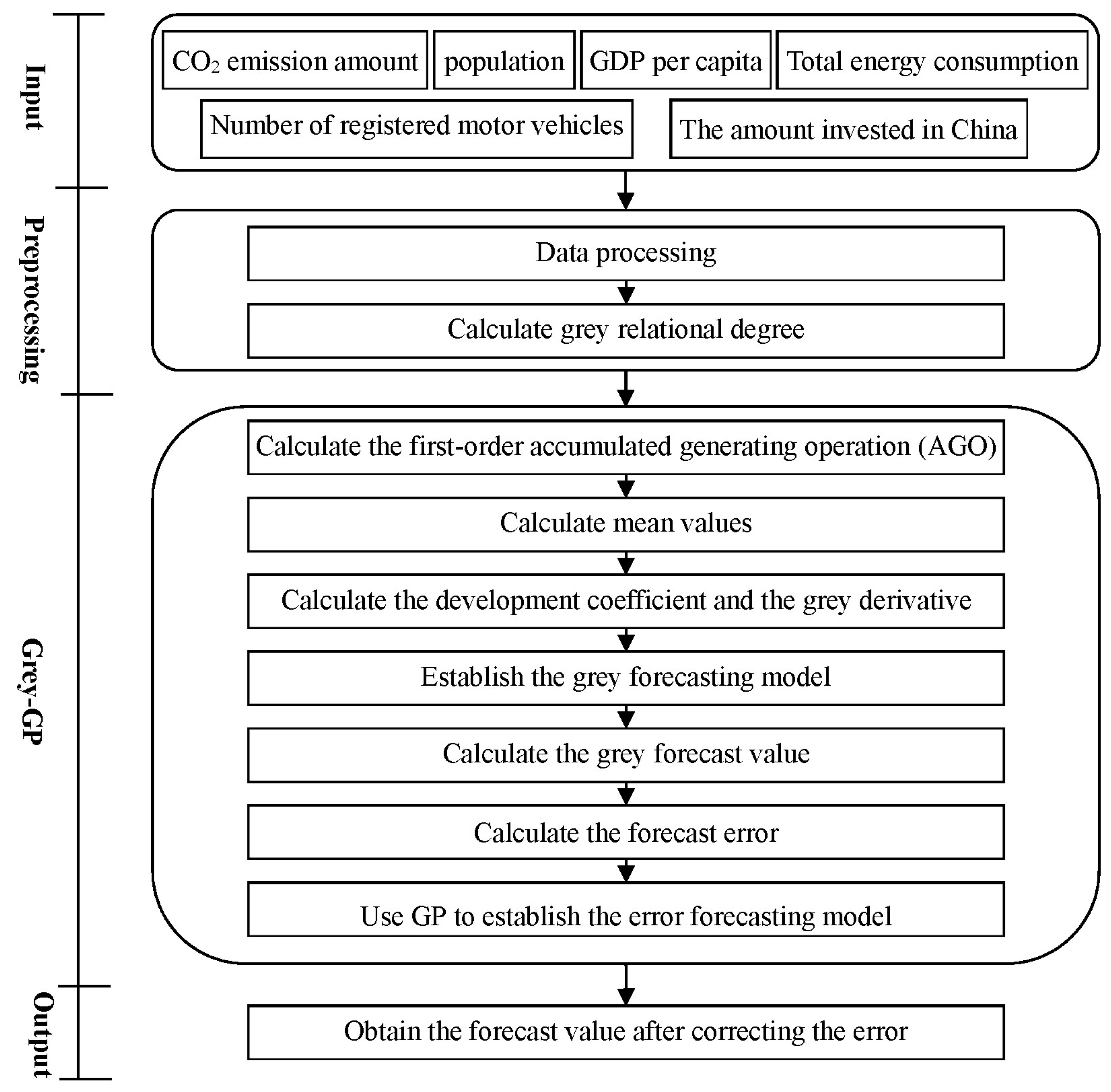
3. Methodology

Most of the forecasting methods commonly used in the previous studies adopted actual observed values to estimate the forecast value and did not consider other factors in the forecasting model. In addition, when the data shows a non-linear trend, the forecast value showed poor performance. To prevent these defects, we propose a mixed multivariable grey forecasting and GP model. This method is divided into two stages, the first stage is the multivariable grey forecasting method GM(1, N), in which the first parameter value 1 represents that the first-order derivative is applied in the forecasting model; and the second parameter represents that there are N − 1 associated series besides the predicted series. GM(1, N) has the advantage that it can introduce factors that can impact the forecast value into the forecasting model and only need four or more samples to accurately make forecasts. However, when the data is a non-linear trend, the grey forecasting model could show poorer forecast values. To improve the forecast accuracy, the second stage combines the grey forecasting with GP to build an error correction model with a lower forecast error.

The detailed framework of the proposed two stages is shown in Figure 1. This study considers multiple factors (e.g., population, GDP per capita, total energy consumption, number of registered motor vehicles, the amount invested in China, and so on) to forecast the amount of CO₂ emissions. First, the data of these factors are input. Then, the data is preprocessed, and then the grey relational analysis is used to calculate the grey relational degree between the primary factor (i.e., CO₂ emissions) and each of the other factors. After sorting the grey relational degrees, the important factors with a high degree of grey relation with CO₂ emissions are selected for later analysis. Then, GM(1, N) considering these selected factors is used to build the forecast model and further calculate the grey forecast value. Then, the error between the actual value and the forecast value is calculated. Then, GP is used to build the error forecast model. The final forecast value is obtained by integrating the forecast value from GM(1, N) and the error correction value from GP, to increase accuracy. The next section introduces the grey relational analysis, multivariable grey forecasting model, and GP used in the framework of the proposed method (Figure 1).

3.1. Grey Relational Analysis

The relation among factors can be evaluated according to similarity or difference among the development trends of factors. Through the grey relational analysis between the primary factor (i.e., carbon emissions in this study) and multiple factors, we can understand the correlation between the two as time or space changes. When system decision and forecast provide usable information or more reliable basis, this type of analysis model can clearly show the correlation between factors. The grey relational analysis procedures are as follows:

• When calculating the grey relation, a time series is established based on the original observed value of each period. Let $X_0(k)$ denote the primary series and $X_i(k)$, i = 1, 2, …, N denote the associated series, where k denotes the index of the period such as week, month, or year:

  $$\begin{array}{l}{X}_0=(X_0(1),X_0(2),\dots ,X_0(k)),\\ X_1=(X_1(1),X_1(2),\dots ,X_1(k)),\\ X_2=(X_2(1),X_2(2),\dots ,X_2(k)),\\ \begin{array}{ccc}& ⋮& \end{array}\\ X_N=(X_N(1),X_N(2),X_N(3),\dots ,X_N(k)),\\ \\ k=1,2,\dots ,m\end{array}$$
• The maximum difference and minimum difference between the primary series and the other associated series are calculated as follows:

  $${\Delta }_{\min }=\underset{\forall j\in i}{\min }\underset{\forall k}{\min }\left|X_0(k)-X_j(k)\right|$$

  (1)

  $${\Delta }_{\max }=\underset{\forall j\in i}{\max }\underset{\forall k}{\max }\left|X_0(k)-X_j(k)\right|$$

  (2)
• The grey relational coefficient $\gamma$ between the primary series and the associated series in period k is calculated as follows:

  $$\gamma (X_0(k),X_i(k))=\frac{{\Delta }_{\min }+\zeta {\Delta }_{\max }}{{\Delta }_{0i}(k)+\zeta {\Delta }_{\max }}$$

  (3)

  where ζ is the identification coefficient; and ${\Delta }_{0i}(k)=\left|X_0(k)-X_i(k)\right|$. Generally speaking, the identification coefficient value should be 0.5. However, to magnify the difference of the results, this value can be adjusted according to the actual need.
• The grey relational degree between the primary series and the associated series is the mean of all grey relational coefficients as calculated as follows:

  $$\gamma (X_0,X_i)=\frac{1}{m}{\displaystyle \sum _{k=1}^m\gamma (X_0(k),X_i(k))}$$

  (4)

The importance level of each factor can be obtained by comparing the grey relational degree between the primary factor and each other factor and then sorting them. The ordering of the grey relational degrees can then be used as the basis for the entire system’s decision making.

3.2. Multivariable Grey Forecasting Method GM(1, N)

In the grey forecasting model, GM(h, n) is a type of dynamic model, where h is the order number of the differential equation that characterizes the dynamic model; and n is the number of variables (i.e., factors in this study). GM(1, 1) and GM(1, N) are the most commonly used modes. The GM(1, 1) model uses the historical data of one variable to forecast the future behavior of the same variable. Differently, the GM(1, N) model has only one behavior variable, but has multiple variables that affect the behavior. Therefore, to consider multiple factors in forecasting carbon emissions, this study method uses GM(1, N).

The GM(1, N) model is introduced as follows: In the grey system, $X_1^0(k)$ is the observed value of the primary factor in period k; and $X_i^0(k)$, i = 2, …, N, is the associated factor.

• After the first-order accumulation generating operation (1-AGO) on the observed series $X_i^{(0)}=(X_i^{(0)}(1),X_i^{(0)}(2),\dots ,X_i^{(0)}(k))$ of each factor i, we obtain $X_i^{(1)}=(X_i^{(1)}(1),X_i^{(1)}(2),\dots ,X_i^{(1)}(k))$ where:

  $$X_i^{(1)}(k)={\displaystyle \sum _{m=1}^k{X}_i^{(0)}(m)}$$

  (5)
• Similar to whitening the GM(1, 1) model to obtain the general differential equation $X^{(0)}(k)+a{z}^{(1)}(k)=b$, the differential equation for the GM(1, N) model is expressed as follows:

  $$X_i^{(0)}(k)+a{z}_1^{(1)}(k)={\displaystyle \sum _{i=2}^N{b}_i{X}_i^{(1)}(k)}$$

  (6)

  where a is the grey development coefficient, which is the major parameter that reflects development trends; b_i is the grey action coefficient corresponding to the associated series i; and the mean series is obtained as follows:

  $$z_i^{(1)}=0.5\cdot x_i^{(1)}(k)+0.5\cdot x_i^{(1)}(k-1),k\ge 2$$

  (7)
• Transform Equation (6) into the following matrix form:

  $$\left[\begin{array}{c}{X}_1^{(0)}(2)\\ X_1^{(0)}(3)\\ ⋮\\ X_1^{(0)}(m)\end{array}\right]=\left[\begin{array}{cccc}-z_1^{(1)}(2)& X_2^{(1)}(2)& \dots & X_N^{(1)}(2)\\ -z_1^{(1)}(3)& X_2^{(1)}(3)& \dots & X_N^{(1)}(3)\\ ⋮& ⋮& & ⋮\\ -z_1^{(1)}(m)& X_2^{(1)}(m)& \dots & X_N^{(1)}(m)\end{array}\right]\left[\begin{array}{c}a\\ b_2\\ ⋮\\ b_n\end{array}\right]$$

  (8)
  The above matrix is solved by the least-squares method to obtain coefficient a and coefficient b_i. Then, $\widehat{\alpha }={\left[\begin{array}{cccc}a& b_2& \cdot \cdot \cdot & b_N\end{array}\right]}^T={(B^{T}B)}^{-1}{B}^{T}Y$ where:

  $$Y=\left[\begin{array}{c}{X}_1^{(0)}(2)\\ X_1^{(0)}(3)\\ ⋮\\ X_1^{(0)}(m)\end{array}\right]\mathrm{and}B=\left[\begin{array}{cccc}-z_1^{(1)}(2)& X_2^{(1)}(2)& \dots & X_N^{(1)}(2)\\ -z_1^{(1)}(3)& X_2^{(1)}(3)& \dots & X_N^{(1)}(3)\\ ⋮& ⋮& & ⋮\\ -z_1^{(1)}(m)& X_2^{(1)}(m)& \dots & X_N^{(1)}(m)\end{array}\right]$$
• We substitute coefficients a and b_i into Equation (6) to obtain the following series:

  $${\widehat{X}}_1^{(1)}(k+1)=[X_1^{(0)}(1)-{\displaystyle \sum _{i=2}^N\frac{b_i}{a}{X}_i^{(1)}(k+1)}]e^{-ak}+{\displaystyle \sum _{i=2}^N\frac{b_i}{a}{X}_i^{(1)}(k+1)}$$

  (9)
• Conduct inverse accumulation generation to obtain the forecast value:

  $${\widehat{X}}_1^{(0)}(k+1)={\widehat{X}}_1^{(1)}(k+1)-{\widehat{X}}_1^{(1)}(k)$$

  (10)

When the forecast value is obtained, the future dynamic status of the factors can be understood. Then, the error series between original values and forecast values is calculated. We then used the GP to estimate the error series, and conduct error correction to improve the accuracy.

3.3. Genetic Programing

GP is a type of automated function production method. Given a set of parameters, GP can automatically find a function that conforms to the parameters. The basic concept is based on GA, which includes reproduction, crossover, and mutation. The difference between GP and GA is that GA is expressed in an encoded string, but GP is expressed as a program tree diagram. Using GA to solve a problem suffers from the solution representation, with a fixed length that restricts the solution searching ability. In addition, it is not intuitive to decode the calculation results. Differently, GP is not limited by a fixed length, and can directly express the calculation results, which makes it easier to understand by decision makers.

The main architecture of GP includes a terminal set and function set. The former expresses variables or constants; and the latter expresses mathematical or calculation symbols (formed from addition, subtraction, multiplication, division, polynomials, trigonometric function, or other types of function). After the two sets are confirmed, it is required to define the fitness function to be optimized, set control parameters, and decide termination conditions of the GP algorithm. Then, GP is used to obtain the optimal function that best conform to actual objectives.

This study uses GP to correct the forecast error between actual values and forecast values. First, GM(1, N) is used to obtain the forecast values, and then calculate the error series:

$$e_i(k)=x_i(k)-{\widehat{x}}_i(k)$$

(11)

Then, GP is used to find the function characterizing the above error series as follows:

$$f({\widehat{e}}_i)=f\left(x_i\left(1\right),x_i(2),\dots ,x_i(k)\right),i=1,2,\dots ,N$$

(12)

The architecture of GP is set as follows: the terminal set is {e_i(1), e_i(2), …, e_i(k)}. The function set is {+, −, ×, /, log, sin, cos, exp}. The fitness function is defined as $\min \left|{\widehat{e}}_i-e_i\right|,$ for i = 1, 2, …, N. That is, the difference between the error estimation value produced by GP and the error obtained from the GM(1, N) model is used to evaluate fitness. The parameters used in GP include the population size, evolution size, the maximal depth for the evolutionary tree, crossover rate, and mutation rate. These parameter values are set through repeated experiments and exploration. The final forecast value is obtained by summing the forecast value ${\widehat{x}}_i(k)$ obtained by GM(1, N) and the forecast error value ${\widehat{e}}_i(k)$ obtained by GP, as calculated as follows:

$${\widehat{x}}_{i-\mathrm{new}}(k)={\widehat{x}}_i(k)+{\widehat{e}}_i(k)$$

(13)

4. Results

This section built a forecasting model and conducted experimental analysis based on the amount of CO₂ emissions in Taiwan, and considered the factors that affect the amount of CO₂ emissions. Among the factors that affect the amount of CO₂ emissions mentioned in the literature review in Section 2 [1,2,3,4], the factors that had a higher correlation with the amount of emissions include population, GDP per capita, total energy consumption, number of registered motor vehicles, and foreign investment.

The experiment in this study used the data of Taiwan as an example. Based on data from the Department of Statistics, Ministry of Economic Affairs, Taiwan, 50% percent of Taiwan’s foreign investment is in China. In addition, the data on the amount of CO₂ emissions from 2000 to 2015 shows that in 2009 the amount of carbon emissions significantly decreased. From the historic events, the cause of the CO₂ emission decrease during that year may be the financial crisis caused by the American subprime mortgage crisis at the end of 2007. At that time, the global stock market reached a new low, and banks in different countries faced collapse. This had a significant impact on Taiwan’s economy. Affected by the financial crisis, economic development encountered obstructions, and factories were closed.

We collected and compiled the amount of CO₂ emissions data and the factors from 2006 to 2011 (the year before Taiwan faced the financial crisis) for the grey relational analysis, as well as compared forecasts from different GM(1, N) models. We also found that growth of the amount of carbon emissions from 2010 to 2014 was gentle. Data showed that Taiwan’s investment in China increased. As manufacturers moved out from Taiwan, this study attempts to investigate whether this movement slowed down the carbon emission growth in Taiwan. This study analyzed and explored carbon emissions during this period. Data on the amount of CO₂ emissions and the factors in Taiwan for the period from 2010 to 2014 (the year when a large number of Taiwan businessmen moved factories to China) were compiled for grey relational analysis. Forecasts of different GM(1, N) models were compared.

In this section, the first subsection compiled the amount of CO₂ emissions and the factor data for the period from 2000 to 2015 for the grey relational analysis. Then, we further consider two periods. The second subsection analyzed the period from 2006 to 2011 (when Taiwan faced the financial crisis), and the third subsection analyzed the period from 2009 to 2015 (when a large number of Taiwan businessmen moved their factories to China). For the grey forecasting model, N = 2, 3, 4, 5, 6 was substituted to compare different GM(1, N) models.

4.1. Forecast and Analysis of the CO₂ Emission Amount in Taiwan

For the factors that affect Taiwan’s amount of CO₂ emissions, we collected data on Taiwan’s population, GDP per capita, total energy consumption, number of registered motor vehicles, and the amount invested in China for the period from 2000–2015, as shown in

Table 2. Various raw data.

Year	Carbon Emission Amount (Gg CO2-Equivalent)	Taiwan’s Population (People)	GDP per Capita (NT$)	Total Energy Consumption (1000 kiloliter of Oil Equivalent)	Number of Registered Motor Vehicles	Amount Invested in China (1000 USD)
2000	20,936	22,276,672	466,598	101,788.10	16,981,890	2,607,142
2001	21,304	22,405,568	454,687	106,381.60	17,422,491	2,784,147
2002	22,109	22,520,776	475,484	111,424.17	17,861,379	6,723,058
2003	23,068	22,604,550	486,018	119,583.41	18,452,827	7,698,784
2004	23,851	22,689,122	514,405	132,607.81	19,132,734	6,939,912
2005	24,520	22,770,383	532,001	133,679.26	19,809,106	6,002,029
2006	25,207	22,876,527	553,851	136,520.00	20,251,086	7,375,197
2007	25,587	22,958,360	585,016	144,192.32	20,652,231	9,961,542
2008	24,463	23,037,031	571,838	139,161.90	21,029,329	10,691,390
2009	23,218	23,119,772	561,636	136,267.54	21,306,396	7,142,593
2010	24,828	23,162,123	610,140	142,501.32	21,650,247	14,617,872
2011	25,345	23,224,912	617,078	138,236.51	22,150,801	14,376,624
2012	24,864	23,315,822	631,142	140,768.47	22,265,065	12,792,077
2013	24,911	23,373,517	652,429	143,135.84	21,477,473	9,190,090
2014	25,104	23,433,753	687,816	147,453.21	21,198,831	10,276,570
2015	26,463	23,483,793	711,310	145,084.20	21,400,897	9,896,793

Data source: Bureau of Energy, Directorate General of Budget, Accounting and Statistics (DGBAS), Department of Household Registration, Ministry of Transportation and Communications (MOTC), and Investment Commission of the Ministry of Economic Affairs (MOEAIC), Taiwan.

. We then applied the grey relational analysis to understand the importance ordering of the factors and the correlation(s) between them. The key to the analysis lay in the correlation coefficient between the factors.

The grey relational degree between the amount of CO₂ emissions and the factors is shown in

Table 3. Grey relational degree between CO₂ emission amount and factors.

	Population	GDP per Capita	Total Energy Consumption	Number of Registered Motor Vehicles	Amount Invested in China
$\gamma (X_0,X_i)$	0.9486	0.9592	0.9377	0.9807	0.5533

, in which the highest correlation of the amount of CO₂ emissions is with the number of registered motor vehicles. The second highest correlation is with the GDP per capita, followed by population, total energy consumption, and amount invested in China. The relational degree between each pair of factors is not significant. The key to the analysis is the correlation ordering between the factors.

The data from 2000–2013 includes a total of 14 sets of observations. The forecast model was built to obtain the simulation value and calculate the simulation value errors. The model forecast value and forecast value error were obtained from 2014 and 2015 data. N = 2, 3, 4, 5 was substituted into GM(1, N) to produce 31 sets of models. Based on the aforementioned method, we separately calculated the models built using different combinations of factors to show their error value and accuracy (

Table 4. Mean error and accuracy rate of Taiwan CO₂ emission amount GM(1, N) model.

Combination of Factors	Simulation Error	Forecast Error	Average Error	Average Accuracy
GM(1, 3) with P, EC	4.45%	2.28%	3.37%	96.63%
GM(1, 4) with G, NV, I	5.29%	1.59%	3.44%	96.56%
GM(1, 2) with NV	4.67%	2.23%	3.45%	96.55%
GM(1, 4) with P, EC, I	4.13%	2.93%	3.53%	96.47%
GM(1, 4) with P, EC, NV	3.91%	3.26%	3.59%	96.41%
GM(1, 5) with P, G, EC, I	4.52%	2.69%	3.61%	96.40%
GM(1, 5) with P, G, EC, NV	4.10%	3.14%	3.62%	96.38%
GM(1, 4) with P, G, EC	4.41%	2.86%	3.63%	96.37%
GM(1, 6) with P, G, EC, NV, I	4.08%	3.24%	3.66%	96.34%
GM(1, 5) with P, EC, NV, I	3.92%	3.41%	3.66%	96.34%
GM(1, 3) with NV, I	5.29%	2.27%	3.78%	96.22%
GM(1, 4) with G, NV, I	4.34%	3.22%	3.78%	96.22%
GM(1, 3) with P, G	5.29%	2.48%	3.88%	96.12%
GM(1, 3) with EC, I	4.38%	3.42%	3.90%	96.10%
GM(1, 5) with P, G, NV, I	5.67%	2.18%	3.93%	96.07%
GM(1, 4) with P, G, I	5.74%	2.20%	3.97%	96.03%
GM(1, 4) with P, NV, I	5.52%	2.48%	4.00%	96.00%
GM(1, 4) with P, G, NV	5.70%	2.40%	4.05%	95.95%
GM(1, 3) with P, NV	5.54%	2.58%	4.06%	95.94%
GM(1, 2) with EC	4.73%	3.58%	4.15%	95.85%
GM(1, 3) with G, EC	4.97%	3.38%	4.17%	95.83%
GM(1, 3) with P, I	5.77%	2.60%	4.18%	95.82%
GM(1, 2) with P	5.77%	2.60%	4.19%	95.82%
GM(1, 4) with EC, NV, I	6.09%	2.91%	4.50%	95.50%
GM(1, 5) with G, EC, NV, I	7.70%	1.45%	4.58%	95.42%
GM(1, 4) with G, EC, NV	4.29%	7.65%	5.97%	94.03%
GM(1, 3) with EC, NV	9.52%	6.60%	8.06%	91.94%
GM(1, 3) with G, NV	5.85%	11.22%	8.53%	91.47%
GM(1, 3) with G, I	25.50%	36.38%	30.94%	69.06%
GM(1, 2) with G	79.85%	61.76%	70.81%	29.19%
GM(1, 2) with I	88.72%	73.91%	81.32%	18.68%

Note: P represents the Taiwan population; G represents GDP per capita; EC represents the total energy consumption; NV represents the number of registered motor vehicles; I represents the amount invested in China from Taiwan.

). Table 4 shows that GM(1, 3) includes the population and the total energy consumption, and its accuracy rate was the highest at 96.63%. Overall, 18 combinations had accuracy higher than 96%. The two combinations with the lowest accuracy were GM(1, 2) using GDP and GM(1, 2) using the amount invested in China. Both had an accuracy rate lower than 30%.

This study applied three types of error evaluation methods as the evaluation indicators of the forecast model. The smaller the error value, the higher the forecast model’s accuracy rate. The first type of error evaluation method is the mean absolute percentage error (MAPE) calculated as follows:

$$\mathrm{MAPE}=\frac{1}{N}{\displaystyle \sum _{k=1}^N\left|\frac{f_k-o_k}{o_k}\right|}\times 100\%$$

(14)

where f_k is the forecast value of period k, and o_k is the original actual value of period k. This method divided the accuracy rate into four levels, as shown in

Table 5. MAPE accuracy level.

	≤ 10%	10%~20%	20%~50%	> 50%
Accuracy level	Highly accurate	Good	Reasonable	Inaccurate

.

The second type of error evaluation method is the mean absolute error (MAE), which uses error to indicate accuracy, and is calculated is as follows:

$$\mathrm{MAE}={\displaystyle \sum _{k=1}^N\frac{\left|f_k-o_k\right|}{N}}$$

(15)

The third type of error evaluation method is the percentage error (PE), which is represented in percentage form. This method can directly compare the difference between the forecast value and actual value, as calculated as follows:

$$\mathrm{PE}=\frac{\left|f_k-o_k\right|}{o_k}\times 100\%$$

(16)

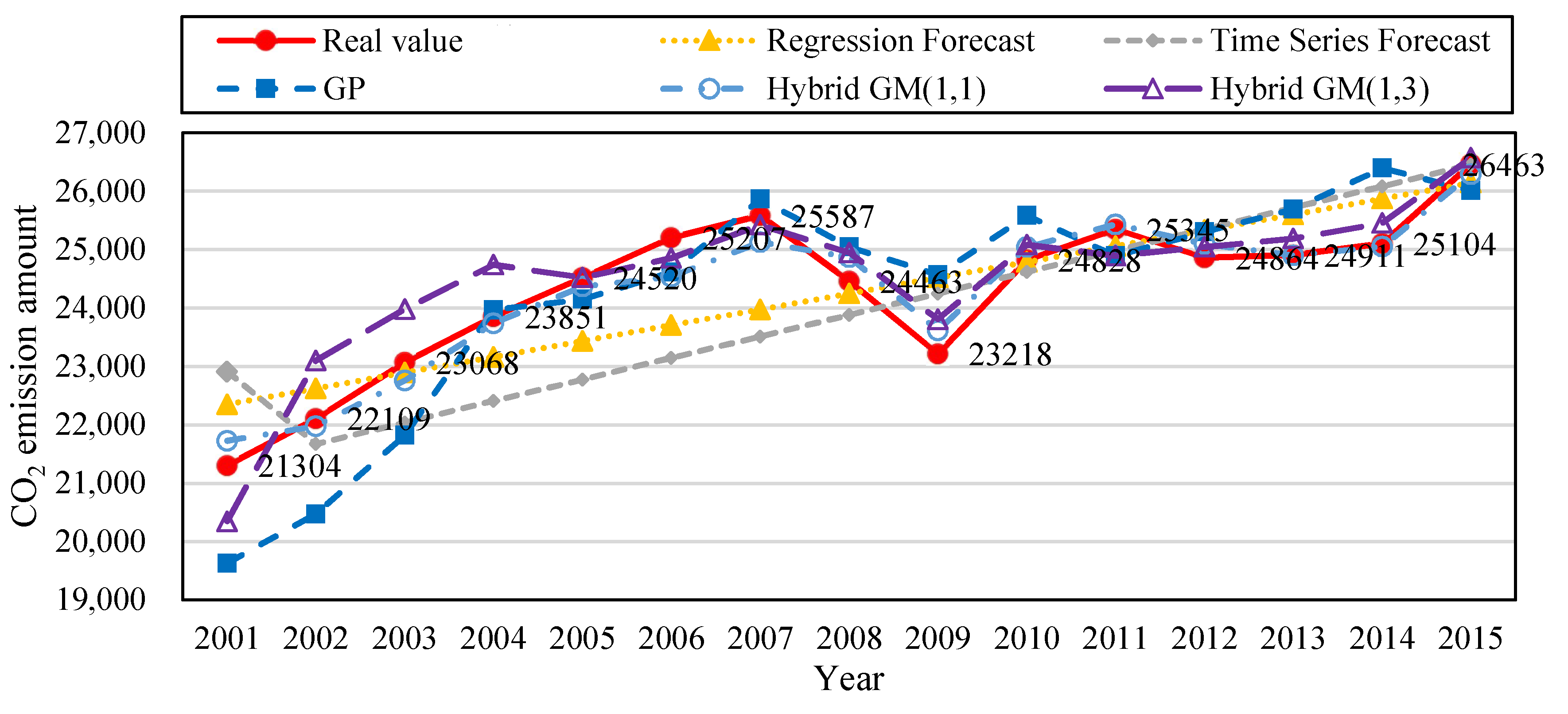
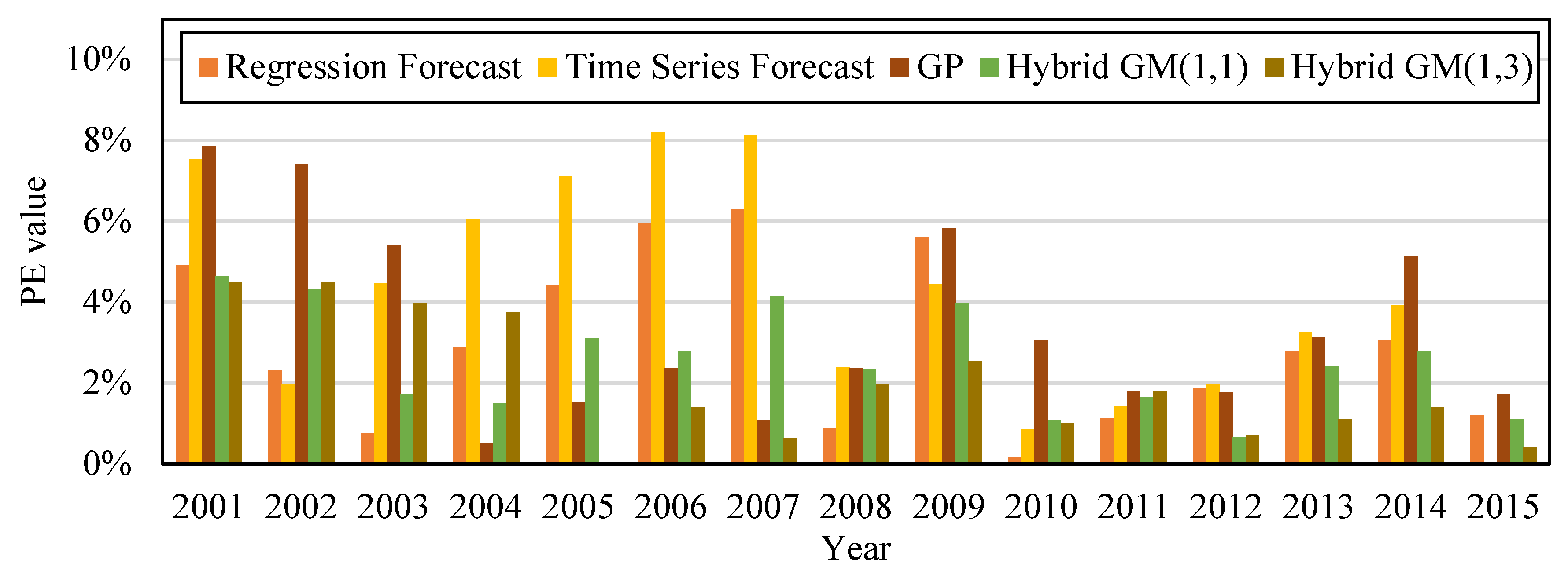
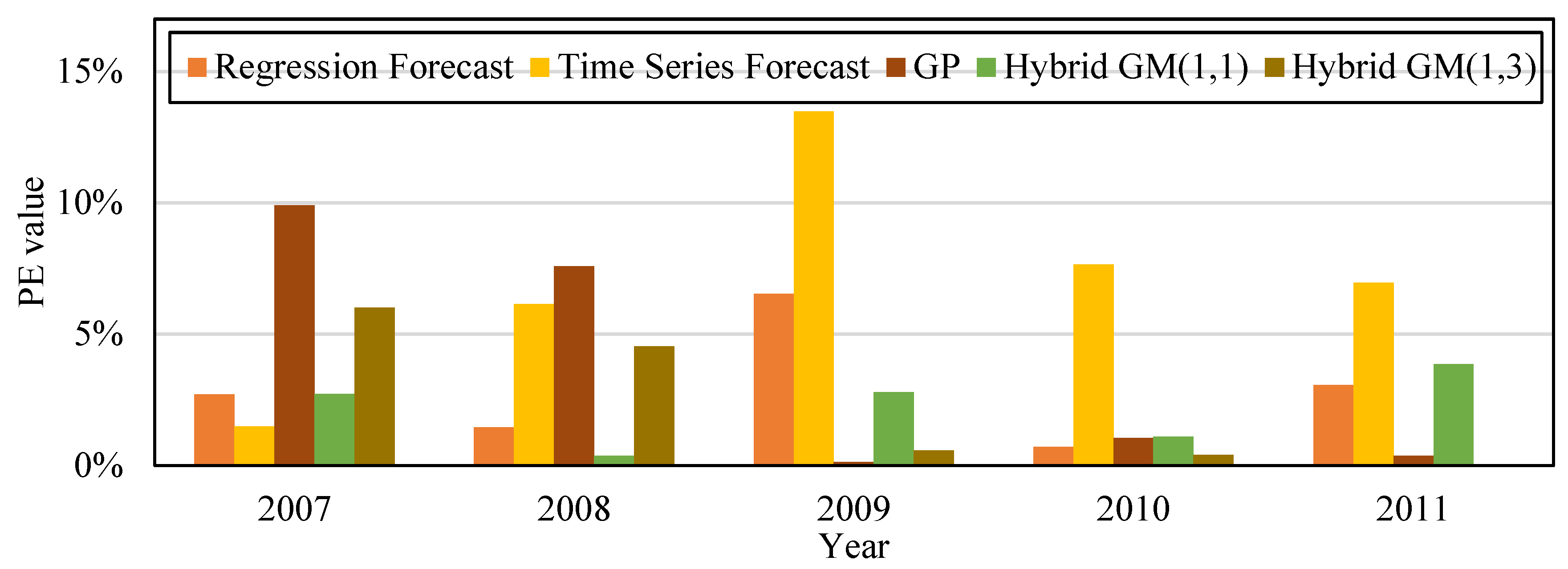
To prove the accuracy of the proposed method, we built the following forecast models based on the data from 2000 to 2015: regression forecast, time series forecast, GP, Hybrid GM(1, 1), and the proposed hybrid GM(1, 3). The built forecast models were trained with 14 sets of data from 2000–2013, and then were tested with two sets of data from 2014–2015.

Table 6. Comparison of five forecast models trained with the data from 2000–2013 and tested with the data from 2014–2015.

Year	Real Value	Regression Forecast		Time Series Forecast		GP		Hybrid GM(1, 1)		Hybrid GM(1, 3)
		Simulation	PE	Simulation	PE	Simulation	PE	Simulation	PE	Simulation	PE
2001	21,304	22,350.4	4.91%	22,907	7.52%	18,842.86	13.06%	21,726.23	4.6%	19,046.65	4.5%
2002	22,109	22,621.3	2.32%	21,672	1.98%	26,202.04	15.62%	21,979.24	4.3%	26,365.75	4.5%
2003	23,068	22,892.2	0.76%	22,040	4.46%	25,144.92	8.26%	22,757.94	1.7%	25,305.06	4.0%
2004	23,851	23,163.0	2.88%	22,408	6.05%	24,723.45	3.53%	23,737.88	1.5%	24,844.14	3.7%
2005	24,520	23,433.9	4.43%	22,776	7.11%	24,437.15	0.34%	24,370.46	3.1%	24,519.58	0.0%
2006	25,207	23,704.8	5.96%	23,144	8.18%	24,515.35	2.82%	24,535.62	2.8%	24,853.90	1.4%
2007	25,587	23,975.7	6.30%	23,512	8.11%	24,867.04	2.90%	25,125.12	4.1%	25,425.72	0.6%
2008	24,463	24,246.6	0.88%	23,880	2.38%	24,708.94	1.00%	24,871.53	2.3%	24,948.51	2.0%
2009	23,218	24,517.4	5.60%	24,248	4.44%	24,651.85	5.82%	23,615.23	4.0%	25,195.36	2.5%
2010	24,828	24,788.3	0.16%	24,616	0.85%	24,948.26	0.48%	25,043.91	1.1%	25,079.83	1.0%
2011	25,345	25,059.2	1.13%	24,984	1.42%	24,819.81	2.12%	25,435.47	1.7%	24,892.17	1.8%
2012	24,864	25,330.1	1.87%	25,352	1.96%	25,000.76	0.55%	25,096.56	0.7%	25,042.46	0.7%
2013	24,911	25,601.0	2.77%	25,720	3.25%	25,147.65	0.94%	24,901.87	2.4%	25,188.18	1.1%
MAPE
(01-13)			3.07%		4.44%		4.42%		2.64%		2.14%
MAE
(01-13)			768.78		1067.38		1079.89		248.67		457.40
2014	25,104	25,871.8	3.06%	26,088	3.92%	25,378.75	1.08%	25,050.47	2.8%	25,453.16	1.4%
2015	26,463	26,142.7	1.21%	26,456	0.03%	25,319.91	4.51%	26,293.30	1.1%	26,573.95	0.4%
MAPE
(14, 15)			2.13%		1.97%		2.80%		2.65%		0.91%
MAE
(14, 15)			544.54		1061.42		708.921		205.09		119.10

shows that the MAPE of regression forecast, time series forecast, GP, Hybrid GM(1, 1), and the proposed hybrid GM(1, 3) during training data was 3.07%, 4.44%, 4.42%, 2.64%, and 2.14%; and their MAE during training data was 768.78, 1,067.38, 1,079.89, 248.67, and 457.399, respectively. Their MAPE during testing data was 2.13%, 1.79%, 2.80%, 2.65%, and 0.91%, respectively; and their MAE during testing data was 544.54, 1,061.42, 708.921, 205.09, and 119.101, respectively. Figure 2 shows the trend of the amount of CO₂ emissions established with the simulation value and forecast value of the five types of forecast models from Table 6. Figure 3 is the bar chart built from the PE values of the five forecast models in Table 6. It can be observed that compared with other forecast models, the method proposed by this study had better accuracy for forecasting the amount of CO₂ emissions.

4.2. Analysis of the Amount of CO₂ Emissions in Taiwan during the Financial Crisis

The financial crisis caused by the American subprime mortgage crisis at the end of 2007 resulted in new lows in the global stock markets. Many banks faced bankruptcy and the crisis produced a significant impact on Taiwan’s economy. As the financial crisis hit, the news often reported factory shutdowns and company layoffs. The unemployment rate hit a historic high, as the labor market rapidly worsened to a level not seen before. To analyze the factors that affected Taiwan’s amount of CO₂ emissions during the financial crisis, we collected data on population, GDP per capita, total energy consumption, number of registered motor vehicles, and the amount invested in China for the period from 2006–2011, as shown in Table 4. We then applied the grey relational analysis to understand the importance of factors and the relational degrees of factors. The key to the analysis is the relational degrees of factors.

The grey relation degrees of all factors was sorted from large to small.

Table 7. Grey correlation of the amount of CO₂ emissions and factors.

	Population	GDP per Capita	Total Energy Consumption	Number of Registered Motor Vehicles	Amount Invested in China
$\gamma \left(X_0,X_i\right)$	0.9476	0.8812	0.9303	0.8946	0.6166

shows that Taiwan’s population has the highest correlation with the amount of CO₂ emissions, followed by total energy consumption, the number of registered motor vehicles, GDP per capita, and the amount invested in China.

Simulation values were obtained from the forecast model built with the data from 2006 to 2010, and the simulation value error was calculated. The model forecast value and forecast value error were obtained from the data in 2011. N = 2, 3, 4, 5 was substituted in GM(1, N) to produce 31 sets of models. Based on the aforementioned method, we separately calculated the models built from different combinations of factors. The error values and accuracy were also calculated, as shown in

Table 8. The mean error and accuracy rate of GM(1, N) model during the financial crisis (i.e., trained with the data from 2007–2010 and tested with the data in 2011).

Combination of Factors	Simulation Error	Forecast Error	Average Error	Average Accuracy
GM(1, 5) with P, EC, NV, I	5.44%	0.26%	2.85%	97.15%
GM(1, 2) G	4.84%	1.02%	2.93%	97.07%
GM(1, 3) G, NV	5.27%	0.61%	2.94%	97.06%
GM(1, 3) G, I	5.11%	0.92%	3.01%	96.99%
GM(1, 3) NV, I	5.54%	0.81%	3.18%	96.82%
GM(1, 2) NV	5.64%	0.93%	3.29%	96.71%
GM(1, 5) P, G, EC, NV	6.20%	0.49%	3.34%	96.66%
GM(1, 3) P, G	5.30%	1.48%	3.39%	96.61%
GM(1, 4) P, EC, I	5.41%	1.61%	3.51%	96.49%
GM(1, 3) P, I	5.43%	1.67%	3.55%	96.45%
GM(1, 4) P, G, EC	5.52%	1.98%	3.75%	96.25%
GM(1, 5) P, G, EC, I	6.95%	0.57%	3.76%	96.24%
GM(1, 3) P, NV	5.98%	1.74%	3.86%	96.14%
GM(1, 4) P, G, I	5.67%	2.06%	3.87%	96.13%
GM(1, 3) G, EC	5.64%	2.21%	3.93%	96.07%
GM(1, 4) G, EC, I	5.65%	2.24%	3.95%	96.05%
GM(1, 4) P, NV, I	5.72%	2.18%	3.95%	96.05%
GM(1, 4) P, G, NV	6.01%	2.18%	4.10%	95.90%
GM(1, 4) EC, NV, I	5.75%	2.47%	4.11%	95.89%
GM(1, 4) G, EC, NV	5.79%	2.44%	4.12%	95.89%
GM(1, 3) EC, NV	5.86%	2.53%	4.19%	95.81%
GM(1, 4) P, EC, NV	5.81%	2.73%	4.27%	95.73%
GM(1, 3) EC, I	6.05%	3.01%	4.53%	95.47%
GM(1, 6) P, G, EC, NV, I	6.98%	2.83%	4.90%	95.10%
GM(1, 2) P	6.91%	3.44%	5.17%	94.83%
GM(1, 2) EC	6.78%	4.41%	5.59%	94.41%
GM(1, 3) P, EC	6.96%	4.71%	5.83%	94.17%
GM(1, 4) G, NV, I	21.27%	19.15%	20.21%	79.79%
GM(1, 2) I	34.1%	36.51%	35.31%	64.69%
GM(1, 5)G, EC, NV, I	56.72%	44.52%	50.62%	49.38%
GM(1, 5) P, G, NV, I	67.22%	48.57%	57.9%	42.1%

Note: P represents the Taiwan population; G represents GDP per capita; EC represents the total energy consumption; NV represents the number of registered motor vehicles; I represents the amount invested in China from Taiwan.

. Results show that GM(1, 5), which included Taiwan’s population, total energy consumption, number of registered motor vehicles, and the amount invested in China had an accuracy rate of 97.15%, which is the combination with the highest accuracy. Among all combinations, three combinations had accuracies higher than 97%, and 14 combinations had accuracies higher than 96%.

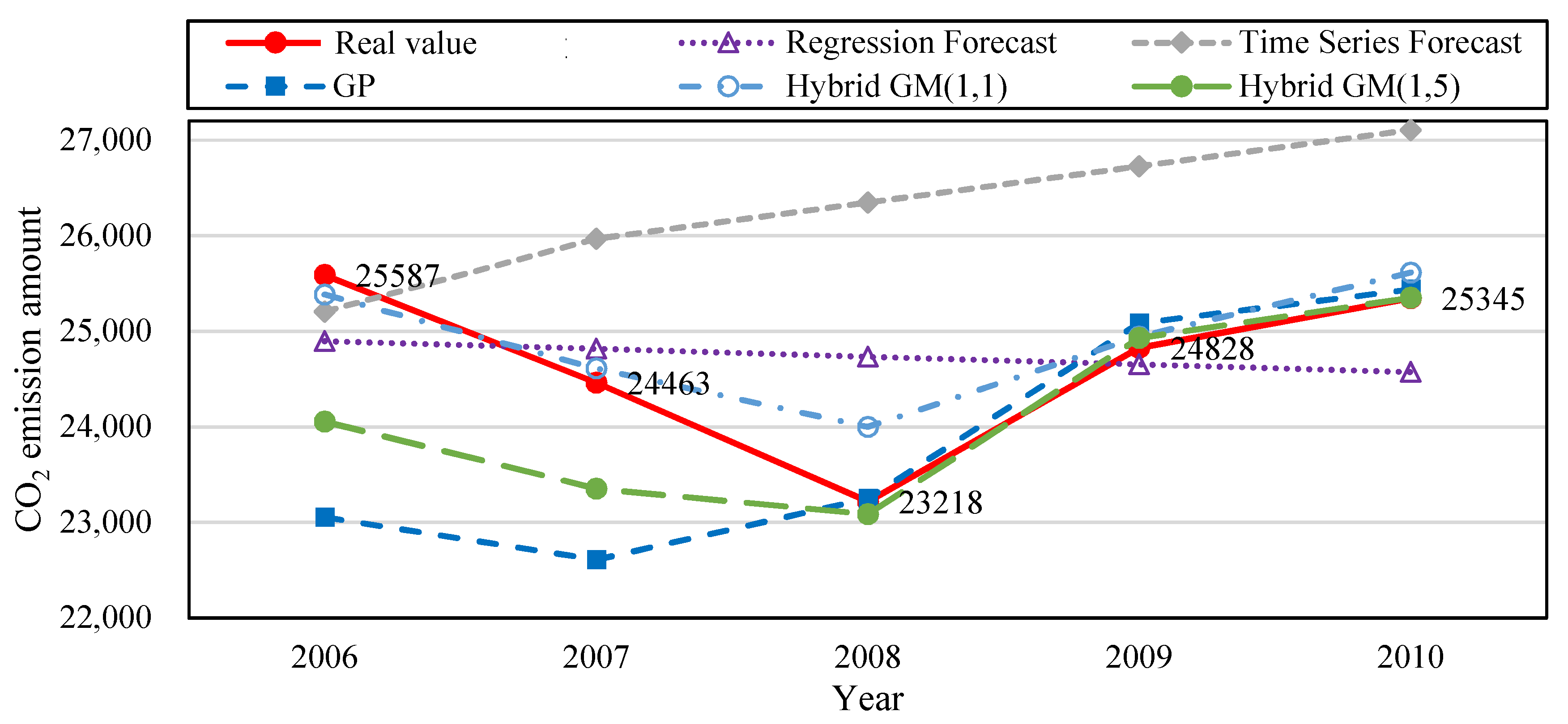
We built the following forecast models based on data from 2006 to 2011: regression analysis forecast, time series forecast, GP, hybrid GM(1, 1), and our proposed hybrid GM(1, 5). Five sets of data from 2006–2010 were used to train the forecast models, and then tested with data from 2011.

Table 9. Comprehensive comparison of forecast model trained with the data from 2007–2010 and tested with the data in 2011.

Year	Real Value	Regression Forecast		Time Series Forecast		GP		Hybrid GM(1, 1)		Hybrid GM(1, 5)
		Simulation	PE	Simulation	PE	Simulation	PE	Simulation	PE	Simulation	PE
2007	25,587	24,896.0	2.70%	25,207	1.49%	23,053.83	9.90%	25,383.70	2.72%	24,052.30	6.00%
2008	24,463	24,815.1	1.44%	25,967	6.15%	22,609.25	7.58%	24,609.06	0.37%	23,354.61	4.53%
2009	23,218	24,734.2	6.53%	26,347	13.48%	23,247.98	0.13%	23,999.04	2.79%	23,085.06	0.57%
2010	24,828	24,653.3	0.70%	26,727	7.65%	25,085.03	1.04%	24,943.91	1.09%	24,927.84	0.40%
MAPE			2.84%		7.19%		4.66%		1.74%		2.88%
(07-10)
MAE			592.80		1728.00		1168.48		250.25		602.46
(07-10)
2011	25,345	24,572.4	3.05%	27,107	6.95%	25,437.31	0.36%	25,614.84	3.86%	25,350.54	0.02%
MAPE			3.05%		6.95%		0.36%		3.86%		0.02%
MAE			592.80		1762		92.31		951.03		5.54

shows that the MAPE during training data for regression analysis forecast, time series forecast, GP, hybrid GM(1, 1), the proposed hybrid GM(1, 5) was 2.84%, 7.19%, 4.66%, 1.74%, and 2.88%, respectively. Their MAE during training data was 592.8, 1728, 1168.48, 250.25, and 602.46, respectively. Their MAPE during testing data was 3.05%, 6.95%, 0.36%, 3.86%, and 0.02%, respectively. The MAE during training data was 592.8, 1762, 92.31, 951.03, and 5.54, respectively. Figure 4 is the CO₂ emission amount trend produced from the simulation value and forecast value of the five forecast models in Table 9 for the financial crisis period. Figure 5 is the bar chart that compares the PE values from the five forecast model from Table 9. The original actual value in the data and chart clearly shows that after the financial crisis occurred in 2008, the amount of CO₂ emissions decreased significantly. CO₂ emissions gradually rose with the revival of the economy. Compared with other forecast models, the proposed model has superior fitness and variability, and is more accurate in forecasting CO₂ emission amount.

4.3. The Impact of Taiwan Businessmen Moving Overseas on Taiwan’s CO₂ Emission Amount

When Taiwan began allowing Taiwan businessmen to invest in China in 1990, the first people to invest in China were from the manufacturing industry and labor-intensive industries. Investments in the manufacturing industry accounted for 90% of all investments in China. China is large and full of resources, so small and medium-size industries can achieve economies of scale in production and sales. In addition, the land, equipment, factory, and labor were cheap in China, which gave small and medium-size companies an advantage in growth. Considering the popularity of investing in China in recent years, we collected factors that impacted CO₂ emissions in Taiwan during the period that Taiwan businessmen were moving overseas. We collected data on population, GDP per capita, total energy consumption, number of registered motor vehicles, and amount invested in China for the period between 2010 and 2014. We then applied grey relational analysis to understand the importance of factors and the relational degree between factors. The key to the analysis is the relational degree between factors. The grey relational degrees of all factors was sorted from large to small.

Table 10. Grey correlation for the amount of CO₂ emissions and factors.

	Population	GDP per Capita	Energy Consumption	Number of Registered Motor Vehicles	Amount Invested in China
$\gamma \left(X_0,X_i\right)$	0.9122	0.8052	0.9266	0.8847	0.5093

shows that Taiwan’s energy consumption has the highest correlation with the amount of CO₂ emissions, followed by population, the number of registered motor vehicles, GDP per capita, and the amount invested in China.

Simulation values were obtained from forecast model built with the data from 2010 to 2013, and the simulation value errors were calculated. Model forecast value and forecast value error were obtained with the data from 2014. N = 2, 3, 4, 5 was substituted in GM(1, N) to produce 31 combinations of factors used in the grey model. Based on the aforementioned method, we separately calculated models built from different factor combinations. The error values and accuracy were also calculated, as shown in

Table 11. Mean error and accuracy rate of the GM(1, N) model during the period when Taiwan businessmen were moving overseas (i.e., trained with the data from 2011–2013 and tested with the data in 2014).

Combination of Factors	Simulation Error	Forecast Error	Average Error	Average Accuracy
GM(1, 4) with P, NV, I	3.77%	0.49%	2.13%	97.87%
GM(1, 4) with G, EC, I	5.98%	0.65%	3.31%	96.69%
GM(1, 4) with P, EC, I	6.58%	0.63%	3.60%	96.40%
GM(1, 3) with G, I	6.34%	1.04%	3.69%	96.31%
GM(1, 4) with EC, NV, I	5.77%	1.88%	3.82%	96.18%
GM(1, 3) with NV, I	5.95%	2.44%	4.19%	95.81%
GM(1, 3) with P, I	7.05%	1.41%	4.23%	95.77%
GM(1, 4) with G, NV, I	6.18%	2.40%	4.29%	95.71%
GM(1, 2) with G	6.11%	2.61%	4.36%	95.64%
GM(1, 5) with P, G, EC, I	6.92%	1.88%	4.40%	95.60%
GM(1, 3) with EC, NV	6.95%	2.43%	4.69%	95.31%
GM(1, 6) with P, G, EC, NV, I	6.04%	3.70%	4.87%	95.13%
GM(1, 2) with P	7.64%	2.68%	5.16%	94.84%
GM(1, 3) with P, EC	7.62%	2.71%	5.17%	94.83%
GM(1, 2) with EC	7.79%	2.54%	5.17%	94.83%
GM(1, 3) with G, NV	7.90%	2.89%	5.39%	94.61%
GM(1, 3) with P, NV	8.09%	2.86%	5.47%	94.53%
GM(1, 3) with EC, I	8.01%	2.99%	5.50%	94.50%
GM(1, 2) with NV	5.43%	6.41%	5.92%	94.08%
GM(1, 3) with G, EC	5.52%	7.96%	6.74%	93.26%
GM(1, 4) with G, EC, NV	11.52%	5.43%	8.47%	91.53%
GM(1, 3) with P, G	11.76%	5.74%	8.75%	91.25%
GM(1, 4) with P, G, NV	12.01%	6.11%	9.06%	90.94%
GM(1, 4) with P, G, EC	12.63%	6.41%	9.52%	90.48%
GM(1, 4) with P, EC, NV	13.26%	7.96%	10.61%	89.39%
GM(1, 4) with P, G, I	19.80%	23.29%	21.54%	78.46%
GM(1, 5) with P, G, EC, NV	30.91%	25.59%	28.25%	71.75%
GM(1, 5) with G, EC, NV, I	22.65%	42.80%	32.73%	67.27%
GM(1, 5) with P, EC, NV, I	55.70%	91.88%	73.79%	26.21%
GM(1, 5) with P, G, NV, I	65.72%	89.3%	77.51%	22.49%
GM(1, 2) with I	67.21%	90.96%	79.09%	20.91%

Note: P represents the Taiwan population; G represents GDP per capita; EC represents the total energy consumption; NV represents the number of registered motor vehicles; I represents the amount invested in China from Taiwan.

. Result show that GM(1, 4), which included Taiwan’s population, number of registered motor vehicles, and amount invested in China had an accuracy rate of 97.87%, which is the highest accuracy. Four combinations had accuracy higher than 96%.

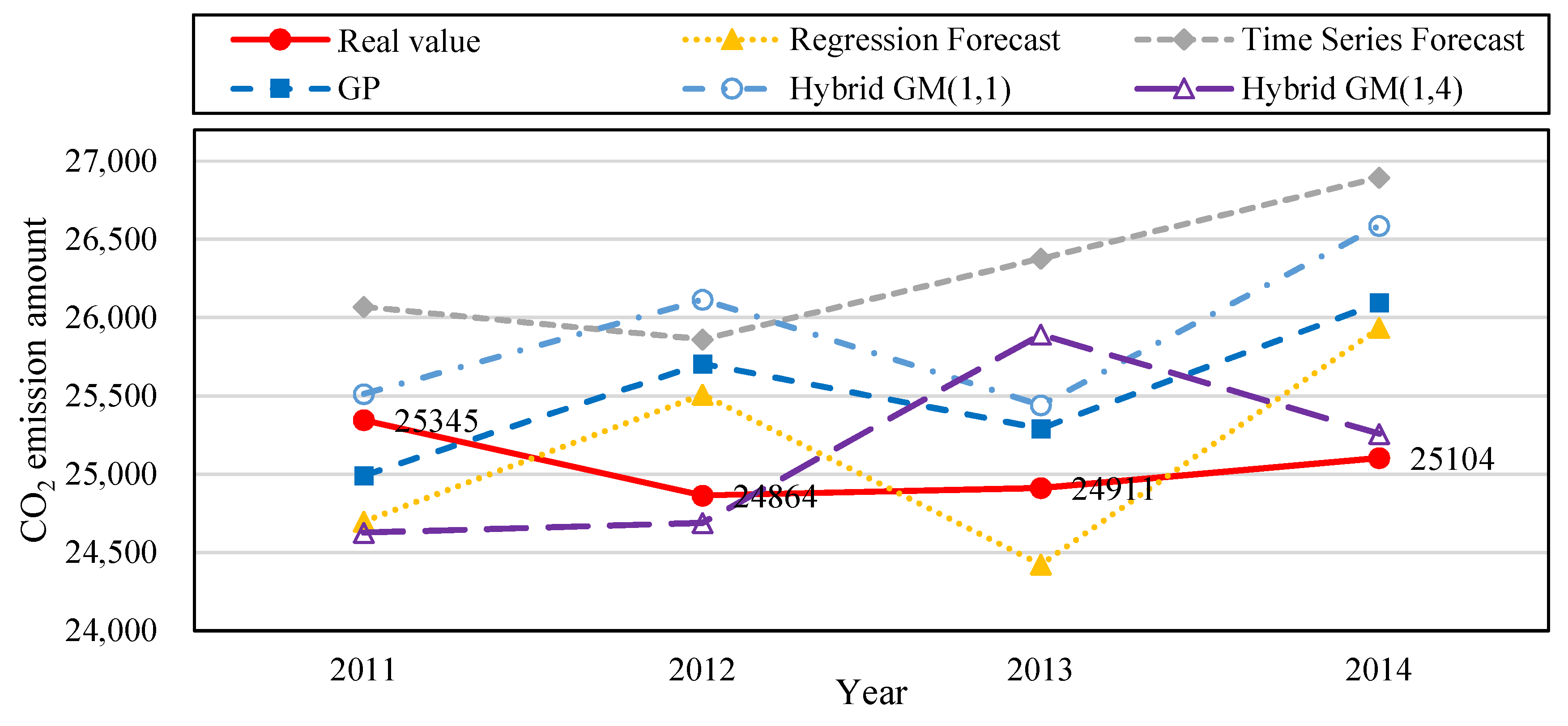
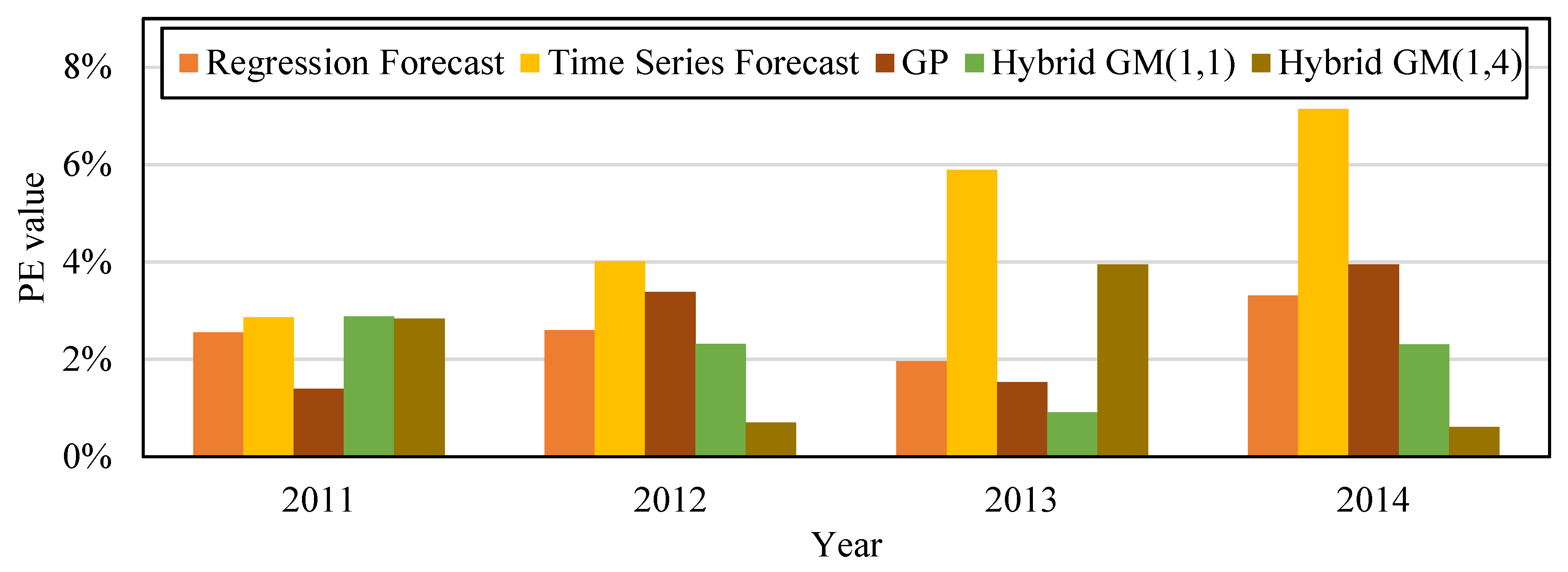
We built the following forecast models based on data from 2010 to 2014: regression forecast, time series forecast, GP, hybrid GM(1, 1), and the proposed hybrid GM(1, 4). Four sets of data from 2010 to 2013 were used to train the forecast models, and then were tested with data from 2014.

Table 12. Comprehensive comparison of forecast model trained with the data from 2011–2013 and tested with the data in 2014.

Year	Real Value	Regression Forecast		Time Series Forecast		GP		Hybrid GM(1, 1)		Hybrid GM(1, 4)
		Simulation	PE	Simulation	PE	Simulation	PE	Simulation	PE	Simulation	PE
2011	25,345	25,286.8	1.85%	25,011	0.74%	23,783.27	6.16%	25,512.63	2.9%	24,626.80	2.8%
2012	24,864	24,698.6	2.55%	26,071	2.86%	24,234.79	2.53%	26,115.29	2.3%	24,690.29	0.7%
2013	24,911	25,510.4	2.60%	25,862	4.01%	25,559.53	2.60%	25,441.51	0.9%	25,893.21	3.9%
MAPE
(11-13)			2.24%		3.38%		3.77%		2.03%		2.49%
MAE
(11-13)			560.1		843.75		946.49		511.5		408.90
2014	25,104	25,934.0	3.31%	26,896	7.14%	25,227.71	0.49%	26,588.1	2.3%	25,257.58	0.6%
MAPE			3.31%		7.14%		0.49%		2.3%		0.61%
MAE			830		1792		123.71		598.43		153.58

shows that the MAPE during training data for the regression forecast, time series forecast, GP, hybrid GM(1, 1), and the proposed hybrid GM(1, 4) was 2.24%, 3.38%, 3.77%, 2.03%, and 2.49%, respectively. Their MAE during training data was 560.1, 843.75, 946.49, 511.5, and 408.9, respectively. Their MAPE during testing data was 3.31%, 7.14%, 0.49%, 2.3%, and 0.61%, respectively. Their MAE during training data was 830, 1792, 123.71, 598.43, and 153.58, respectively. Figure 6 is the trend if the amount of CO₂ emissions produced with the simulation value and forecast value of the five forecast model in Table 12 for the period when Taiwan businessmen were moving overseas. Figure 7 is the bar chart that compares the PE values from the five forecast models in Table 12. The original actual value in the data and chart clearly shows that the amount of CO₂ emissions in 2010 dropped after Taiwan businessmen moved overseas. Compared with other forecast models, the proposed model has superior fitness and variability, and is more accurate in forecasting the amount of CO₂ emissions.

5. Discussion

The result of this study shows that a large N value (i.e., number of factors are considered) may not make the GM(1, N) forecast produce more accurate forecast values. Thus, the value of N is not related to accuracy. A possible reason is that too many factors considered in the model have interactions with one another, so that they can produce offsets or additive effects that decrease the forecast accuracy. Furthermore, in the grey relational analysis that affects the amount of CO₂ emissions, the scale of the relational degree of factors does not have a significant influence on forecast accuracy. Hence, by repeatedly experimenting with different combinations of factors, we were able to determine the combination with the highest accuracy. The difference between the proposed forecast model and the classical GM(1, 1) or other conventional forecast methods is that the proposed forecast model not only considers the time change in the original data, but also considers the factors that are reflected on the actual value. We also used GP to conduct error value correction to avoid only considering changes in original data. This is because when drastic change occurs to a factor, it could result in an excessive forecast error.

The experimental analysis was divided into three environments (for total amount of CO₂ emissions during the financial crisis period and when Taiwan businessmen moved overseas) for comparison. The experiment results show that the method proposed in this study has higher accuracy rate and better adaption to different environmental changes compared to other methods. The main experiment conclusions are as follows:

• Our experimental results showed that the amount of carbon emissions began to drop significantly after 2006. Therefore, the forecast error for those few years also increased significantly. From previous history and news, at that time, global stock markets were at historic lows, and banks in different countries faced bankruptcy. Taiwan was affected by the financial crisis caused by the American subprime mortgage crisis. The experiment scenario was focused on the carbon emission forecast and analysis for Taiwan during the financial crisis period. The most accurate model for forecasting Taiwan’s CO₂ emission amount during this period considered the following factors: population, total energy consumption, number of registered motor vehicles, and the amount invested in China.
• The experiments also found that the growth of the amount of carbon emissions from 2010 to 2014 was gentle. Data shows that when Taiwan’s investment in China grew and manufacturers moved overseas, there is a possibility that this slowed down carbon emissions in Taiwan. Therefore, we analyzed and explored that period. For the period from 2010 to 2014, the most accurate Taiwan amount of CO₂ emission forecast model considered the following factors: Taiwan’s population, number of registered motor vehicles, and the amount invested in China.

6. Conclusions

This work has proposed an approach that integrates multivariable grey forecasting and GP to consider multiple factors to forecast carbon emissions. Multivariable grey forecasting model is suitable for making predictions based on multiple factors with only four or more samples; and GP is used to create the error correction model for the prediction error of multivariable grey forecasting model. The performance of the proposed approach was tested on a case study for forecasting the carbon dioxide emissions in Taiwan from 2000 to 2015. The experimental result showed that the proposed approach with three factors (i.e., population, energy consumption, and carbon emissions) performed best among various combinations of six factors in this case. Note that the proposed approach applied in different examples may conclude that considering a different number of factors performs best. In addition, compared with previous approaches, the proposed approach also showed higher accuracy.

The possible limitation of the proposed approach is as follows. Inherited from the limitation of grey forecasting as indicated in a lot of previous literature (e.g., [7,20,21]), the proposed method includes the grey forecasting method that adopts the least-squares method in estimation, so the predictions of the proposed method may be biased when the data samples have a lot of noise or show a sudden peak/valley owing to some sudden events or external factors. For example, when some country or region starts to implement a series of regulations and methods to prohibit or reduce CO₂ emissions in some year, the data that year may have a large drop. However, those regulations and methods may not be effective or stable in the following years, and hence the data of these years may demonstrate great vibration. Most forecasting methods suffer from this kind of noisy data.

In the future, we will use different types of data, such as electricity consumption and market sales data, for forecasting. The use of different types of problems and parameters will be more challenging for the mixed multivariable grey forecasting model designed in this study. Because factors for actual values are directly reflected in the forecast model, we can determine what kind of problem is suitable for what type of mathematical model. If we can put this model to good use, we can effectively solve instability and improve problem solving efficiency.

References

- Zakarya, G.Y.; Mostefa, B.; Abbes, S.M.; Seghir, G.M. Factors Affecting CO2 Emissions in the BRICS countries: A panel data analysis. Procedia Econ. Financ. 2015, 26, 114–125. [Google Scholar] [CrossRef]
- Wu, L.; Liu, S.; Liu, D.; Fang, Z.; Xu, H. Modelling and forecasting CO2 emissions in the BRICS (Brazil, Russia, India, China, and South Africa) countries using a novel multivariable grey model. Energy 2015, 79, 489–495. [Google Scholar] [CrossRef]
- Wang, T.; Li, H.; Zhang, J.; Lu, Y. Influencing factors of carbon emission in China’s road freight transport. Procedia-Soc. Behav. Sci. 2012, 43, 54–64. [Google Scholar] [CrossRef]
- Xu, B.; Lin, B. Differences in regional emissions in China’s transport sector: Determinants and reduction strategies. Energy 2016, 95, 459–470. [Google Scholar] [CrossRef]
- Belbute, J.M.; Pereira, A.M. An alternative reference scenario for global CO2 emissions from fuel consumption: An ARFIMA approach. Econ. Lett. 2015, 136, 108–111. [Google Scholar] [CrossRef]
- Aydin, G. The Development and validation of regression models to predict energy-related CO2 emissions in Turkey. Energy Sources Part B Econ. Plan. Policy 2015, 10, 176–182. [Google Scholar] [CrossRef]
- Deng, J.L. Grey Prediction and Decision; Huazhong University of Science and Technology: Wuhan, China, 1986. [Google Scholar]
- Wang, Y.; Chen, L.; Kubota, J. The relationship between urbanization, energy use and carbon emissions: Evidence from a panel of Association of Southeast Asian Nations (ASEAN) countries. J. Clean. Prod. 2016, 112, 1368–1374. [Google Scholar] [CrossRef]
- Hammoudeh, S.; Nguyen, D.K.; Sousa, R.M. Energy prices and CO2 emission allowance prices: A quantile regression approach. Energy Policy 2014, 70, 201–206. [Google Scholar] [CrossRef]
- Sohag, K.; Begum, R.A.; Abdullah, S.M.S.; Jaafar, M. Dynamics of energy use, technological innovation, economic growth and trade openness in Malaysia. Energy 2015, 90, 1497–1507. [Google Scholar] [CrossRef]
- Kivyiro, P.; Arminen, H. Carbon dioxide emissions, energy consumption, economic growth, and foreign direct investment: Causality analysis for Sub-Saharan Africa. Energy 2014, 74, 595–606. [Google Scholar] [CrossRef]
- Bastola, U.; Sapkota, P. Relationships among energy consumption, pollution emission, and economic growth in Nepal. Energy 2015, 80, 254–262. [Google Scholar] [CrossRef]
- Wang, Y.; Li, L.; Kubota, J.; Han, R.; Zhu, X.; Lu, G. Does urbanization lead to more carbon emission? Evidence from a panel of BRICS countries. Appl. Energy 2016, 168, 375–380. [Google Scholar] [CrossRef]
- Alam, M.M.; Murad, M.W.; Noman, A.H.M.; Ozturk, I. Relationships among carbon emissions, economic growth, energy consumption and population growth: Testing Environmental Kuznets Curve hypothesis for Brazil, China, India and Indonesia. Ecol. Indic. 2016, 70, 466–479. [Google Scholar] [CrossRef]
- Salahuddin, M.; Gow, J. Economic growth, energy consumption and CO2 emissions in Gulf Cooperation Council countries. Energy 2014, 73, 44–58. [Google Scholar] [CrossRef]
- Tang, C.F.; Tan, B.W. The impact of energy consumption, income and foreign direct investment on carbon dioxide emissions in Vietnam. Energy 2015, 79, 447–454. [Google Scholar] [CrossRef]
- Koza, J.R. Genetic Programming: On the Programming of Computers by Means of Natural Selection; MIT Press: Cambridge, MA, USA, 1992; Volume 1. [Google Scholar]
- Castelli, M.; Trujillo, L.; Vanneschi, L.; Popovič, A. Prediction of energy performance of residential buildings: A genetic programming approach. Energy Build. 2015, 102, 67–74. [Google Scholar] [CrossRef]
- Kovačič, M.; Šarler, B. Genetic programming prediction of the natural gas consumption in a steel plant. Energy 2014, 66, 273–284. [Google Scholar] [CrossRef]
- Wang, Z.-X.; Ye, D.-J. Forecasting Chinese carbon emissions from fossil energy consumption using non-linear grey multivariable models. J. Clean. Prod. 2010, 142, 600–612. [Google Scholar] [CrossRef]
- Wu, L.; Gao, X.; Xiao, Y.; Yang, Y.; Chen, X. Using a novel multivariable grey model to forecast the electricity consumption of Shandong Province in China. Energy 2018, 157, 327–335. [Google Scholar] [CrossRef]
- Hamzacebi, C.; Karakurt, I. Forecasting the energy-related CO2 emissions of Turkey using a grey prediction model. Energy Sources Part A Recovery Util. Environ. Eff. 2015, 37, 1023–1031. [Google Scholar] [CrossRef]
- Meng, M.; Niu, D.; Shang, W. A small-sample hybrid model for forecasting energy-related CO2 emissions. Energy 2010, 64, 673–677. [Google Scholar] [CrossRef]
- Dangerfield, B.J.; Morris, J.S. Top-down or bottom-up: Aggregate versus disaggregate extrapolations. Int. J. Forecast. 1992, 8, 233–241. [Google Scholar] [CrossRef]
- Zarnikau, J. Functional forms in energy demand modeling. Energy Econ. 2003, 25, 603–613. [Google Scholar] [CrossRef]
- Xiao, B.; Guo, P.; Mu, G.; Yan, G.; Li, P.; Cheng, H.; Li, J.; Bai, Y. A spatial load forecasting method based on the theory of clustering analysis. Phys. Procedia 2012, 24, 176–183. [Google Scholar]
- Sbrana, G.; Silvestrini, A. Forecasting aggregate demand: Analytical comparison of top-down and bottom-up approaches in a multivariate exponential smoothing framework. Int. J. Prod. Econ. 2013, 146, 185–198. [Google Scholar] [CrossRef]
- Tra, T.V.; Thinh, N.X.; Greiving, S. Combined top-down and bottom-up climate change impact assessment for the hydrological system in the Vu Gia-Thu Bon River Basin. Sci. Total Environ. 2018, 630, 718–727. [Google Scholar] [CrossRef] [PubMed]
- Lawrence Berkeley National Laboratory. Capabilities of Energy Efficiency Standards (EES) Group. Available online: https://ees.lbl.gov/capabilities (accessed on 7 November 2018).
- Pacific Northwest National Laboratory. Research for Secure, Sustainable Energy. Available online: https://energyenvironment.pnnl.gov (accessed on 7 November 2018).
- McNeil, M.A.; Letschert, V.E.; de la Rue du Can, S.; Egan, C. Acting Globally: Potential Carbon Emissions Mitigation Impacts from an International Standards and Labeling Program; Technical Report LBNL-2331E; Lawrence Berkeley National Laboratory: Berkeley, CA, USA, 2009. [Google Scholar]
- Schein, J.; Letschert, V.; Chan, P.; Chen, Y.; Dunham, C.; Fuchs, H.; McNeil, M.; Melody, M.; Strattron, H.; Williams, A. Methodology for the National Water Savings and Spreadsheet: Indoor Residential and Commercial/Institutional Products, and Outdoor Residential Products; Technical Report LBNL-2001015; Lawrence Berkeley National Laboratory: Berkeley, CA, USA, 2017. [Google Scholar]
- Carvallo, J.; Larsen, P.; Sanstad, A.; Goldman, C. Load Forecasting in Electric Utility Integrated Resource Planning; Technical Report LBNL-1006395; Lawrence Berkeley National Laboratory: Berkeley, CA, USA, 2016. [Google Scholar]
- Kholod, N.; Evans, M. Black Carbon Emissions from Diesel Sources in Russia; Technical Report PNNL-25754; Pacific Northwest National Laboratory: Berkeley, CA, USA, 2016. [Google Scholar]
Figure 1.
The framework of the proposed method.
Figure 2.
Comparison of forecast values of the five forecast models trained with the data from 2000–2013 and tested with the data from 2014–2015.
Figure 3.
Comparison of PE values of the five forecast models trained with the data from 2000–2013 and tested with the data from 2014–2015.
Figure 4.
Comparison of the five forecast models trained with the data from 2007–2010 and tested with the data in 2011.
Figure 5.
Comparison of PE values of the five forecast models trained with the data from 2007–2010 and tested with the data in 2011.
Figure 6.
Comparison of forecast values of the five forecast models trained with the data from 2011–2013 and tested with the data in 2014.
Figure 7.
Comparison of PE values of the five forecast models trained with the data from 2011–2013 and tested with the data in 2014.