
Tree Based Approaches for Predicting Concrete Carbonation Coefficient
by
 , and
, and
Shreenivas Londhe
1, 
Preeti Kulkarni
1,
Pradnya Dixit
1,
Ana Silva
2,* ,
,
Rui Neves
3 and
and
Jorge de Brito
2 1
Vishwakarma Institute of Information Technology, Pune 411048, India
2
Civil Engineering Research and Innovation for Sustainability, Instituto Superior Técnico, University of Lisbon, Av. Rovisco Pais, 1049-001 Lisbon, Portugal
3
Civil Engineering Research and Innovation for Sustainability, ESTBarreiro, Polytechnic Institute of Setúbal, R. Américo da Silva Marinho, 2839-001 Lisbon, Portugal
*
Author to whom correspondence should be addressed.
Appl. Sci. 2022, 12(8), 3874; https://doi.org/10.3390/app12083874
Submission received: 14 February 2022
/
Revised: 5 April 2022
/
Accepted: 9 April 2022
/
Published: 12 April 2022
(This article belongs to the Special Issue Diagnostics and Monitoring of Steel and Concrete Structures)
Abstract
:Carbonation is one of the critical durability issues in reinforced concrete structures in terms of their structural integrity and safety and may cause the fatal deterioration and corrosion of steel reinforcement if ignored. Many researchers have performed a considerable number of studies to predict the carbonation of concrete structures. However, it is still challenging to predict the carbonation depth or carbonation coefficient, as they depend on various factors. Therefore, creating a model that can learn from available data using Data Driven Techniques (DDT) is a step forward in this research field. This study provides new approaches to predict the carbonation coefficient of concrete through Model Tree (MT), Random Forest (RF) and Multi-Gene Genetic Programming (MGGP) approaches. With 827 case studies, the predicted models can be seen as a function of a set of conditioning factors, which are statistically significant in explaining the carbonation mechanism. The results obtained through MT, RF and MGGP were compared with those obtained through Multiple Linear Regression (MLR), Artificial Neural Networks (ANNs) and Genetic Programming (which were previously developed). The results reveal that the MT, RF and MGGP perform better than the previous models. Moreover, the MT technique displays its output in terms of series of equations, RF as multiple trees and MGGP in form of a single equation, which are more user-friendly and applicable in practice.
1. Introduction
Carbonation is one of the major causes of deterioration in reinforced concrete structures [1]. Carbonation can reduce the alkalinity of concrete, thereby making it lose the protection of steel, which is a prerequisite for concrete reinforcement corrosion in the common atmospheric environment. The carbonation of concrete is a natural phenomenon that is commonly defined as the chemical reaction between carbon dioxide (CO2) and cement hydration products such as Ca (OH)2 and calcium–silicate–hydrate (C-S-H). The process of concrete carbonation begins at exposed surfaces immediately upon exposure to CO2, and carbonation rates increase for poor quality, porous concretes and grouts. The consumption of Ca (OH)2 reduces the concrete pH to levels where thin oxides film around the steel surface, which protects it from corrosion, becomes unstable, allowing steel corrosion onset [2,3]. Conventionally, concrete carbonation depth at a given time under steady-state conditions can be fairly predicted by Fick’s second law of diffusion in which the significant parameters are claimed to be the water/cement (w/c) ratio, binder constituents and content and the exposure conditions (e.g., relative humidity) [1,2,3,4,5]. These factors can cause the concrete carbonation coefficient to vary a great deal, as they influence the pore system of hardened concrete (affected by w/c ratio), the amount of Ca (OH)2 to react with CO2 (affected by binder type and content), the dissolution of Ca (OH)2, which is required for it to react with CO2 (affected by relative humidity), and the concentration of CO2 at the concrete surface [5,6]. Developing a holistic and accurate carbonation prediction model is a challenging task, as it is difficult to mathematically describe the several phenomena that occur and, most of all, their interactions. Various theoretical and experimental studies have been carried out to estimate the concrete carbonation depth [7,8,9] and most of them are focused on the estimation of the carbonation rate, through a carbonation coefficient based on the Fick’s second law of diffusion [5]. Even so, it is still difficult to build a prediction model for carbonation depth that can describe all conditions of concrete carbonation.
New age techniques to develop models were defined to describe the complex behaviour of the carbonation coefficient. Data Driven Techniques (DDT) such as Artificial Neural Networks (ANNs) and Genetic Programming (GP), among others, have been used to predict the carbonation depth and carbonation coefficient. Carbonation depth prediction through neural networks (NNs), using the acknowledged input parameters, has been tried [4]. Diffusion coefficients of CO2 were estimated through a neural network algorithm, confirming the decrease in the diffusion coefficient with the increase of relative humidity (RH) and with the decrease of the w/c ratio [10]. Neural network and genetic programming were used to predict the carbonation coefficient and strength of concrete with a correlation coefficient of 0.90 and higher [11]. ANNs have been used for the analysis of the corrosion of steel in concrete to quantify the chloride diffusion in concrete, and it was found that the predictions given by the NNs were adequate [12,13]. Kewalramani and Gupta [14] conducted a study for the prediction of the compressive strength of concrete, using multiple regression analysis and ANNs. Deep neural network architectures provide capabilities to learn hierarchical features from the dataset while providing a more efficient representation than more classic models, improving the generalisation capability of the models [15]. A study by Brusaferria et al. [16] presented a novel probabilistic method for forecasting day-ahead electricity prices based on Bayesian deep learning and deployed a Bayesian inference framework introducing probability distributions over neural network weights and a Gaussian likelihood function. Bayesian linear regression is seen as a suitable tool to revise and update design codes; e.g., the creep correction coefficients are estimated using Bayesian linear regression [17]. Tesfamariam and Martín-Pérez [18] proposed the implementation of a Bayesian Belief Network model for carbonation-induced corrosion of reinforced concrete, which highlighted the impact of various exposure conditions on the rate of carbonation ingress and the potential for reinforcing steel.
Therefore, new models to describe the complex behaviour of the concrete carbonation coefficient still have to be defined, aiming at improving the reliability concerning corrosion prevention. The recent DDTs of Model Tree (MT) and Random Forest (RF) can be suitable vehicles for this task owing to their learning ability from the available data. Carbonation depth has been predicted by adopting decision trees such as the regression tree, bagged ensemble and reduced bagged ensemble regression tree, with excellent performance and understanding of the influential variables [19]. The carbonation depth of concrete using Gene Expression Programming (GEP) was modelled and validated by Murat et al. [20] using the six parameters that predominantly control the carbonation depth of concrete. Currently, there is a trend to carry out concrete mix design and concrete strength prediction through RF and Multi-Gene Genetic Programming (MGGP) [21,22].
In the studies presented so far, no agreement on the way that the carbonation coefficient should be determined has been found. As concrete carbonation depends on many factors and the interactions between them, the modelling of carbonation depth evolution is indeed a complex task. Multiple Linear Regression (MLR) models developed earlier (by some of the authors) displayed a satisfactory performance that can still be improved. Due to the linear nature of MLR, this technique was not capable of modelling the nonlinear relationship between RH and carbonation, and thus the sample analysed was then divided into two subsamples, and two different models were developed: one for an RH of 70% or less and one for an RH higher than 70%. This calls for the use of DDTs such as MT (with M5 Algorithm as splitting criterion), RF and MGGP. The major advantage of these techniques lies in their method of presenting the output and understanding the influential variables. Model Tree displays the output in the form of series of equations, RF in the form of trees and MGGP as equations. The respective outputs are the main innovation of the current work, along with the understanding of the influential parameters in all the techniques. This understanding of the influential parameters gives the researcher more insight into the problem of selecting the most suitable variables and subsequently the models. The current study is a horizontal extension of the studies performed using MLR [23], ANNs and GP [11]. Models are developed to predict the carbonation coefficient of concrete with relevant input parameters, and the performance of the models is compared with that of the existing models [11,23]. The techniques used for this study are Model Tree with M5 Algorithm (MT), Random Forest (RF) and Multi-Gene Genetic Programming (MGGP).
The next section presents a brief introduction of these DDTs, followed by details of the data used in the model development. The methodology adopted for creating the prediction models is discussed further. The results along with the discussion are presented in the subsequent section. This article ends with concluding remarks.
2. Tree Based Modelling Techniques
In the current study, MT, RF and MGGP techniques are grounded on the tree-based approach. Tree-based models use decision trees to present how different input variables can be used to predict a target value and can be used for both classification and regression problems. The basic advantage of tree-based models is that decision trees are easy to understand and interpret, and outcomes can be easily explained. Splitting variables into branches and combining the predictions can aid in maximising information gain and thus obtaining better predictions. The techniques used in the current study are Model Tree with M5 Algorithm (MT), Random Forest (RF) and Multi-Gene Genetic Programming (MGGP).
2.1. Model Tree (MT)
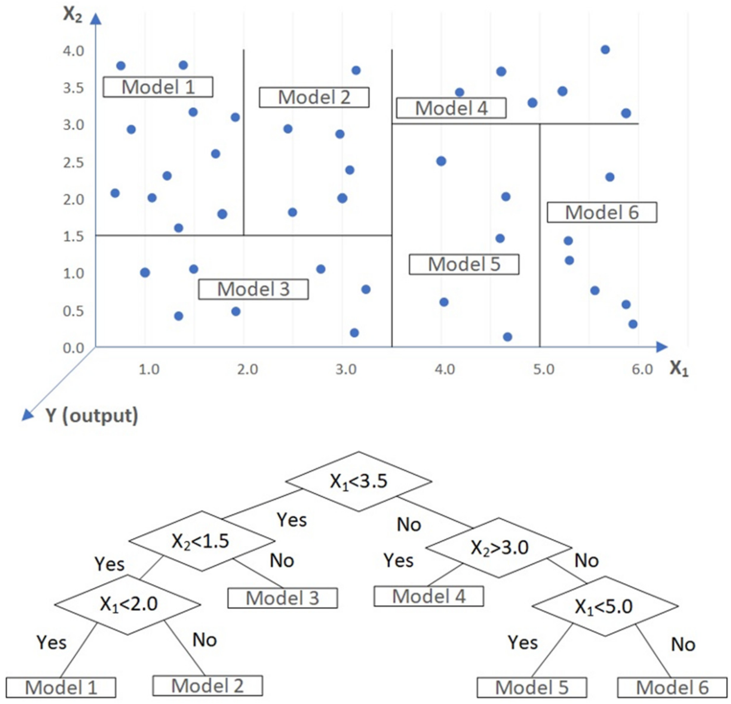
The M5 Model Tree algorithm, used as a splitting criterion, was originally established by Quinlan in 1992 [24]. MT combines a conventional decision tree with the possibility of generating linear regression functions at the leaves. The M5 tree is a piecewise linear model, standing between linear models such as ARIMA (Autoregressive Integrated Moving Average) and nonlinear models as ANNs. Smoothing and pruning is performed to the trees to overcome the over-fitting problem. For decision tree, the splitting criterion is based on the standard deviation error reduction of the values in the subset T of the training data that reaches a particular node (which is an analogue of entropy). For further details of M5 Model Tree, readers are directed to [24,25]. The figure below shows how the M5 algorithm is used for inducing a Model Tree [24] in the present study. A typical Model Tree is shown in Figure 1.
2.2. Random Forest (RF)
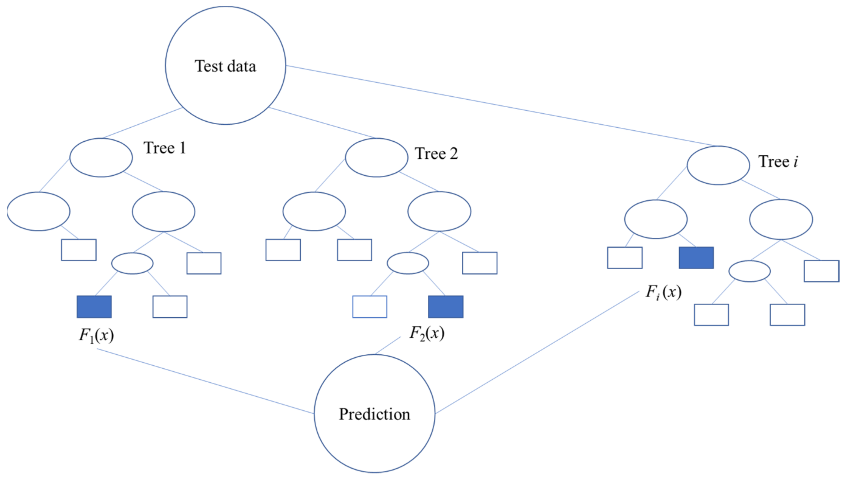
Random Forest is a non-parametric and semi-unsupervised algorithm within the decision tree family, encompassing a collection of uncorrelated trees to generate predictions for regression and classification purposes [26]. It combines bagging and ensemble learning theory with the random subspace method. This method allows the combination of multiple decision trees to obtain the output, instead of only depending on individual decision trees. Random Forest applies multiple decision trees as base learning models. One can randomly perform row and feature sampling from the dataset forming sample datasets for every model (bootstrapping [27]). Random Forest is a classifier involving a compendium of tree-structured classifiers: {h(x, Θi), i = 1 …}, where {Θi} are independent and similarly scattered random vectors and each tree forms a unit vote for the most popular class of input x. The splitting continues until the error goal is met. A bootstrap re-sampling is applied to sample the initial data and create a set of training samples. Each training sample randomly includes the relevant attributes across random subspace techniques to build the decision tree. The optimal result is achieved by voting or averaging method. The analysis of the variable importance in modelling the behaviour of response variables is feasible with RF, using variable importance metrics in two stages [27,28]. Figure 2 shows a Random Forest regression for a typical model.
Feature importance analysis is also an interesting characteristic of RF. Breiman [27] also refers to permutation importance, which quantifies the significance of a variable based on the standard accuracy (classifier) or R2 coefficient (explanatory variable) by evaluating the validation set or the out-of-bag (OOB) samples through the RF. The importance of that variable is the difference between the starting point and the decrease in overall accuracy or R2 affected by transposing the column, and the results are more reliable [27,28]. The higher the value of out-of-bag, the more important the input [29]. The relative position of a variable used as a decision node in a tree establishes the comparative significance of that variable for the prediction of the explanatory variable.
2.3. Multi-Gene Genetic Programming (MGGP)
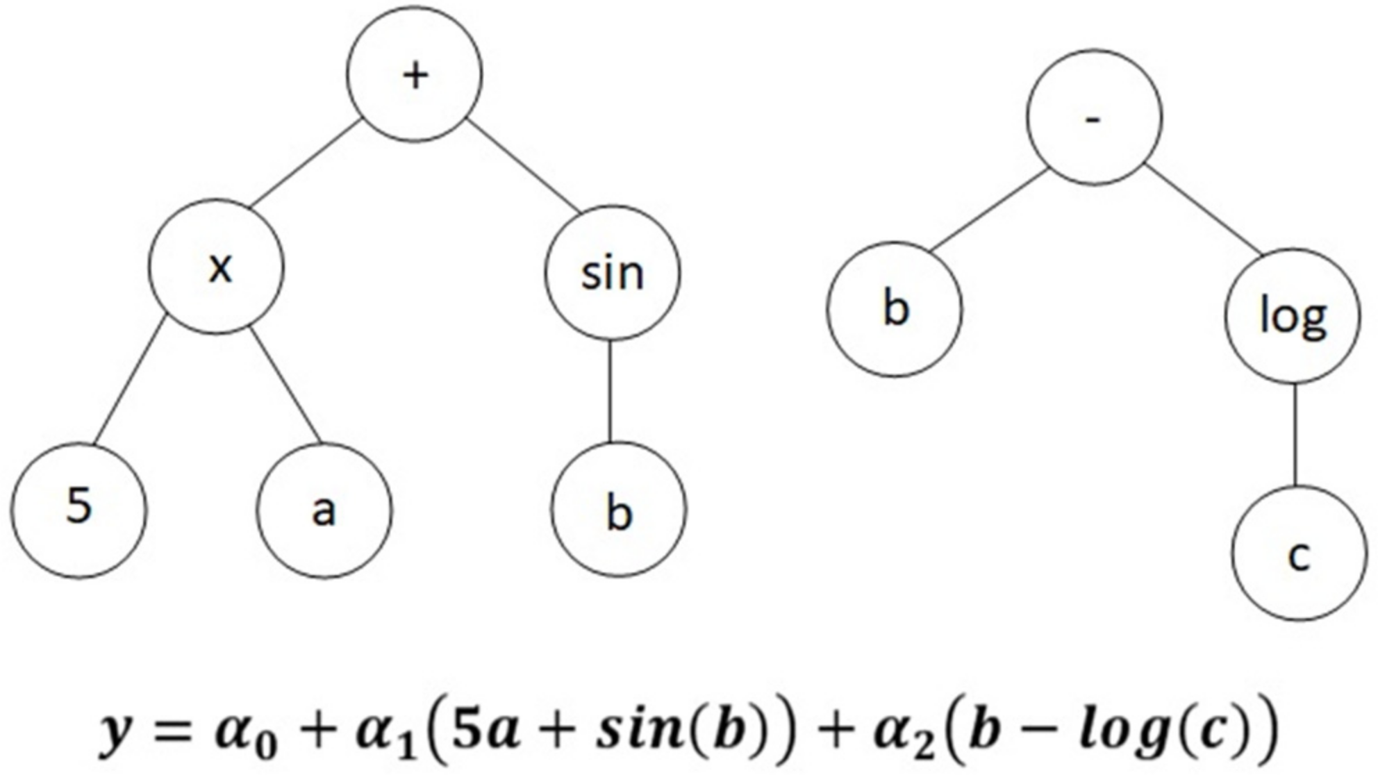
Genetic programming (GP), usually represented by a tree structure, is a machine learning method that is biologically inspired. To perform a task, GP evolves equations or computer programmes and then breeds together the best performing trees to create a new population. Cross-over, mutation and reproduction are the genetic operations used in GP [30]. MGGP, a variant of GP, consists of one or more traditional trees known as genes [31]. Genes are acquired incrementally by individuals in order to improve fitness (e.g., to reduce a model’s sum of squared errors on a data set). The overall model is a weighted linear combination of each gene. Multigene symbolic regression can be implemented using GPTIPS toolbox for Matlab [32,33]. The resulting pseudo-linear model can capture non-linear behaviour. Forcing the transformations to be low order (by restricting the GP tree depth) allows the evolution of accurate, relatively compact mathematical models of predictor–response (input–output) data sets, even when there is a large number of input variables. For example, the multigene model shown in Figure 3 predicts an output variable using the input variables x1, x2 and x3. This model structure contains non-linear terms (e.g., the hyperbolic tangent) but is linear in the parameters with respect to the coefficients a0, a1 and a2. In practice, the user specifies the maximum number of genes, Gmax, a model is allowed to have and the maximum tree depth, Dmax, any gene may have and therefore can exert control over the maximum complexity of the evolved models. In particular, it was found that enforcing stringent tree depth restrictions (i.e., maximum depths of four or five nodes) often allows the evolution of relatively compact models that are linear combinations of low-order non-linear transformations of the input variables.
A Multi-Gene Genetic Programming-based model automatically evolves a mathematical expression in a symbolic form, which can be analysed further to find which variables affect the final prediction and in what trend, and this is the unique aspect of the technique [23]. To provide the identification of input variables that are significant to the output, graphical input frequency analysis of single model or of a user-specified fraction of the population is used [34].
3. Materials and Methods
3.1. Data Used in the Study
As stated earlier, this work is an extension of previous ones and is intended to predict the carbonation coefficient and strength of concrete using Multiple Linear Regression [23], Artificial Neural Networks and Genetic Programming [11]. Therefore, the same data collated from 17 studies (827 values) found in the literature are used. These encompass data from concrete mixes with different types of binder and binder contents, different water/binder ratios and compressive strengths, as well as types of curing and workability. Approximately half of the data concern concrete in service conditions, i.e., natural exposure, whereas the remaining data concern concrete subjected to accelerated carbonation conditions (laboratory CO2 enriched environment). To ensure that the complete data of all variables could be used to determine the value by default, the missing values in any variable were taken as the mean value of the respective [23]. The checking of the data was carried out, and the outliers (points more than three standard deviations away from the mean value of the respective variable) were removed. Further details of the data can be found in [23], while a summary using variable abbreviations is shown in Table 1. These input parameters are the same as those considered in [23], which were selected according to the analysis of variance technique.
For the variable “Exposure class” (X), the value of 1 means that the results concern an exposure to an environment that causes concrete to be permanently dry (e.g., building interior) or permanently wet (e.g., totally immersed). The value of 2 is for concrete exposed to environments with moderate humidity (e.g., concrete in open air structures sheltered from rain). Finally, the value of 3 stands for results from concrete exposed to dry–wet cycles (e.g., concrete in open air structures not sheltered from rain) and for concrete with long periods in contact with water (e.g., rainwater drainage systems).
Various methods of pre-processing data are used by various researchers, such as rescaling, binarising or standardising the data using Gaussian distribution. One of the commonest problems in pre-processing data is missing values. One way of dealing with this is eliminating the variables with missing values, only using the variables with complete data. Despite its simplicity, this approach has several disadvantages, namely because, on several occasions, the dataset is reduced to an insufficient size [35]. Therefore, different methods have been developed to deal with missing values. Simple imputation and multiple imputation are the most common approaches [23]. Here, the missing predictor values are replaced by the mean value of the variable under analysis, considering the physical meaning of the mean value for the reliability of the predictions. Based on this approach, the complete data of the variable can be used to estimate the value by default [23]. The data were carefully analysed, and the outliers for each model to be developed in this study are removed. In this study, all the points whose standard deviation values relative to the average were higher than three were considered influential.
It is widely accepted that the carbonation rate increases with the relative humidity (RH) until a threshold value, beyond which it starts to decrease, becoming virtually nil when concrete becomes saturated [23]. In [23], the sample was divided in two sub-samples, using as a splitting criterion an RH of 70% This procedure was used to allow the use of linear functions. Then, two distinct linear models, instead of a single model, were developed. This study intends to overcome this limitation, proposing a single model to predict the concrete carbonation coefficient for each approach, based on the whole sample. Moreover, the herein proposed models are supposed to provide more accurate predictions, founded on their capability of learning and generalising through behaviour patterns. Furthermore, the models proposed in this study aim at providing a single equation that can be easily used in practice, providing a more transparent model when compared with ANNs [11], which are usually seen as “black boxes”. Additionally, the range of relative humidity found in the samples from which the models are developed is from 50% to 90%, which matches the interval where the higher carbonation rates occur [36].
3.2. Methodology Adopted
To predict the carbonation coefficient (k), the factors affecting the carbonation of concrete were considered. The data mentioned in the previous section were used, and three models were developed using MT, RF and MGGP—one for each tree-based approach. These global models eliminate the use of different models for different humidity levels. The data characteristics of MT, RF and MGGP models are as shown in Table 1.
Model Tree models were developed in WEKA, software version 3.9, developed by University of Waikato, New Zealand [37], and the M5P algorithm developed by Quinlan [24] was used. Random Forest was developed in Python through Jupyter notebook (a web-based interactive computing platform). For RF, the number of trees was selected between 100 and 500, and the bagging iterations and the tree size were selected, anticipating that these were those that yielded the best performance by a low Mean Square Error (MSE). Multi-Gene Genetic Programming was developed in Matlab 2017 using GPTIPS-2 (an open-source toolbox for MGGP). Readers are referred for features of GPTIPS to [31,32]. The Root Mean Square Error (RMSE) function was adapted for error minimisation during runs [31,32]. The parameters were selected as those that yielded the best performance of the models. A large population and generations were assessed to find models with minimum error. The programs were run until the specified number of generations was reached. The allowable number of genes and tree depth were, respectively, set to optimal values as trade-offs between the running time and the complexity of the evolved solutions [31,32]. The best MGGP models were chosen based on providing the best fitness value on the training data as well as the simplicity of the models [32]. These settings in RF and MGGP were based on existing knowledge about the predictive modelling of other data sets of similar size, and so they may not be optimal. The MGGP parameters and their settings are as shown in Table 2.
Variable or parameter importance is also a distinctive feature of the current work. The influential parameters in MT can be highlighted through the values of the standardised coefficients of the parameters, while in RF and MGGP, these can be shown through the variable/parameter permutation importance and the input frequency, respectively. The parameter influence analysis enhances the concept understanding of the algorithm and aids in its validation.
In this investigation, 70% of the data were used for model calibration, while the remaining 30% were used for testing. The model calibration stops when the error in the validation dataset starts increasing—a phenomenon known as over fitting. Statistical metrics such as the correlation coefficient (r), Mean Absolute Error (MAE) and Root Mean Square Error (RMSE) were used to assess models’ performance [38]. High prediction accuracy was expected for lower error statistics (RMSE, MAE), while the opposite was valid for the correlation coefficient. Further, the degree by which RMSE exceeded MAE was an indicator of the extent to which outliers (or variance in the differences between the modelled and observed values) existed in the data [38,39,40]. The results of the models (for testing data set) were also evaluated graphically in the form of scatter plots and hydrograph.
4. Results and Discussion
This section presents the developed models and their performance in testing (i.e., for 30% of the unseen data) and discusses the results.
The number of rules (equations) developed for MT is 6. Figure 4 displays the decision tree of the model and the identification of the leaves’ equations, with these being presented in Equation (1).
Concerning the MT model, when new data are presented, the first step is to analyse the CO2 content, i.e., to check whether CO is ≤3 or >3. If CO is >3, the next branch is selected, and it is again determined whether the CO value is ≤15 or >15. If it is ≤15, the LM 4 equation can be used for the prediction of k. Each variable at each node is analysed by estimating the expected decrease in error. The variable that is selected for separating maximises the expected error reduction at that node. The decision criteria rely on CO2 levels, w/b ratios and compressive strength, corresponding to their higher significance. Furthermore, despite the empirical/statistical nature of the model, it is interesting to notice a positive association of k with w/b ratio and with CO2 content, while the association between k and RH is varying, which is in tune with the fundamental knowledge on concrete carbonation. In general, the negative influence of X and fc is observed through their negative coefficients.
Random Forest (RF) has the unique characteristic of splitting the data randomly and building decision trees and further bagging or averaging the values. This feature of RF stands out in these models’ families and can be also stated as non-linear modelling technique. Random Forest displays the output in terms of the regression trees developed. Random Forest has a unique characteristic of splitting the data randomly and building decision trees and further bagging or averaging the values. This feature of RF stands out in these models’ families and can be also stated as a non-linear modelling technique.
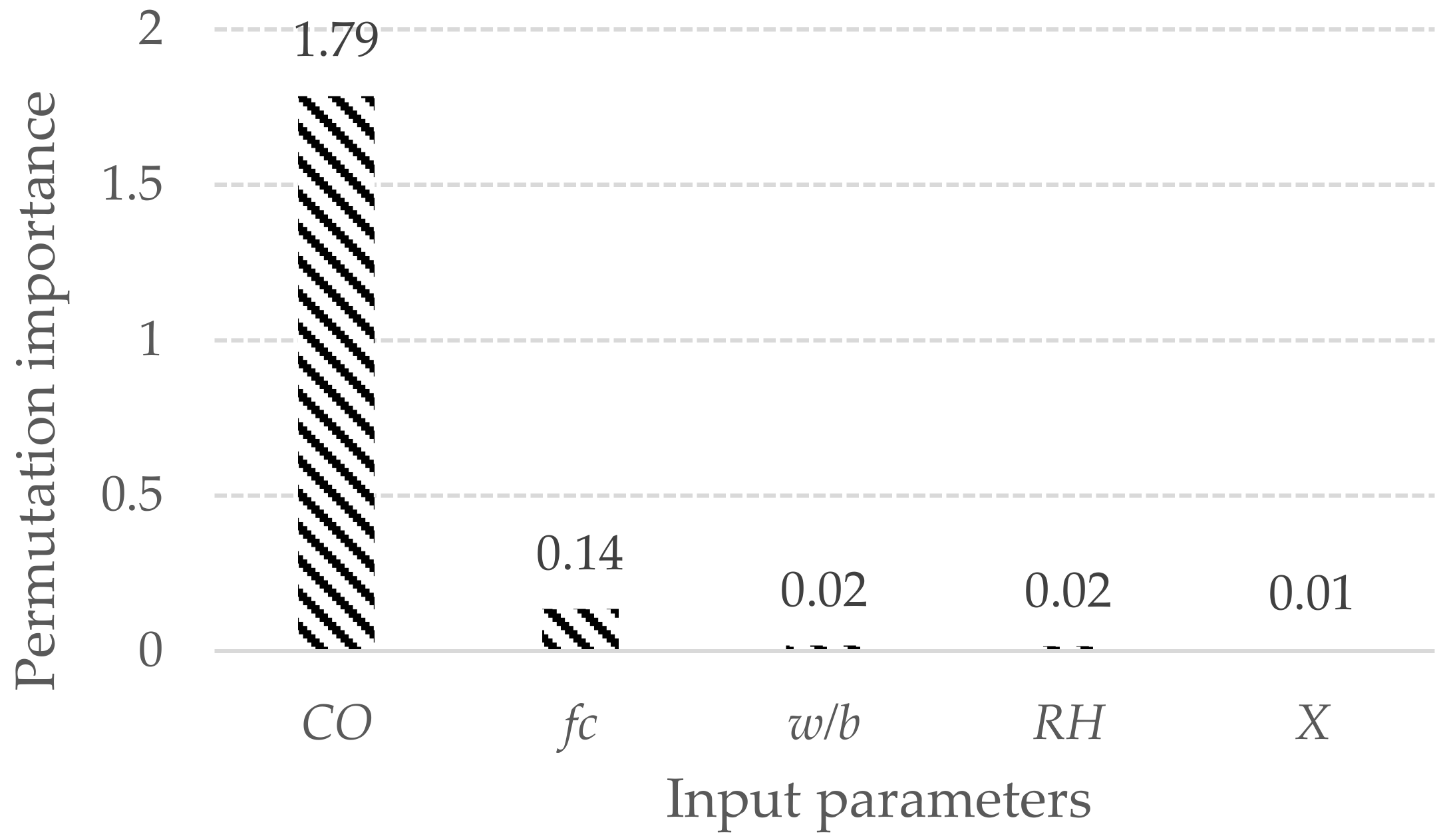
The splitting starts with the randomly selected parameters and determines which parameter value would lead to the “best split” i.e., the least MSE (mean squared error) as its objective or cost function, which needs to be minimised—in this case MSE. The output values at the end of each tree are subjected to averaging. Such a regressor can be useful for a set of equally well-performing models in order to offset their individual weaknesses and can also be called ensemble prediction. RF has the characteristic of the selection of parameters that are highly influential in predicting the output. The permutation feature importance is defined as the reduction in a model result when a single variable value is arbitrarily rearranged. This approach unplugs the connection between the explanatory variable and the response variable; consequently, the decrease in the model ranking reveals how much the variation of the model is explained by that variable. This technique is model-agnostic and can be applied several times, testing various combinations of the explanatory variable [27]. Figure 5 shows the permutation importance of the RF model parameters, where the higher importance of CO is followed by fc, which is in accordance with the fundamental knowledge of the concept.
The third technique of study, MGGP, was employed to develop the MGGP model. The MGGP algorithm merges the model architecture choice proficiency of GP with the variable estimation ability of conventional regression to describe the nonlinear interactions [41,42].
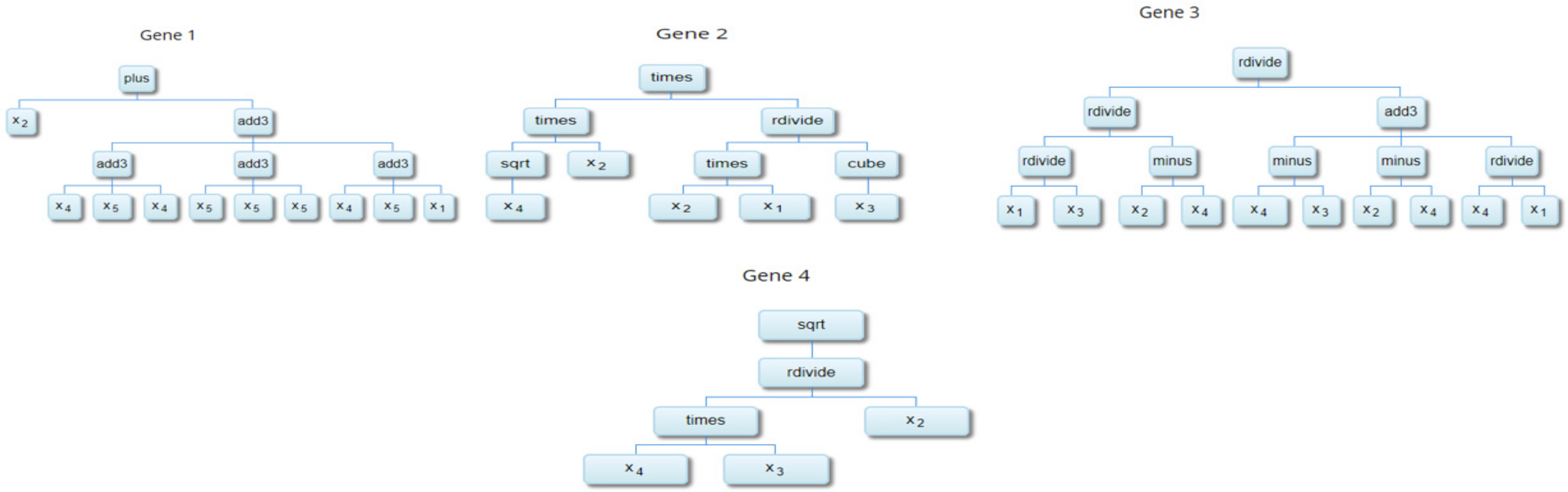
Figure 6 shows the expressional trees developed for the MGGP model. The trees are combined using different weights of genes. Table 3 summarises the equations developed from the trees (genes) and the weights of each gene.
The solution is given by a linear sum of the outputs and a bias value, the weights of which are shown in Table 3. Using the least squares method, the weight related to each tree is determined by minimising the goodness-of-fit error between the model and the training set [38]. The regression equation developed by MGGP is as shown in Equation (2).
The standalone equation, besides being user-friendly, also reflects the importance of each parameter by its inclusion in the equation. GP has a unique characteristic in which the parameter that does not contribute significantly to prediction is removed. MGGP also displays the importance feature in prediction through input frequency analysis. The importance parameter CO has prominently been seen to be followed by w/b, fc, RH and X parameters. This input frequency analysis (Figure 7) also adheres to the fundamental knowledge on the concrete carbonation process.
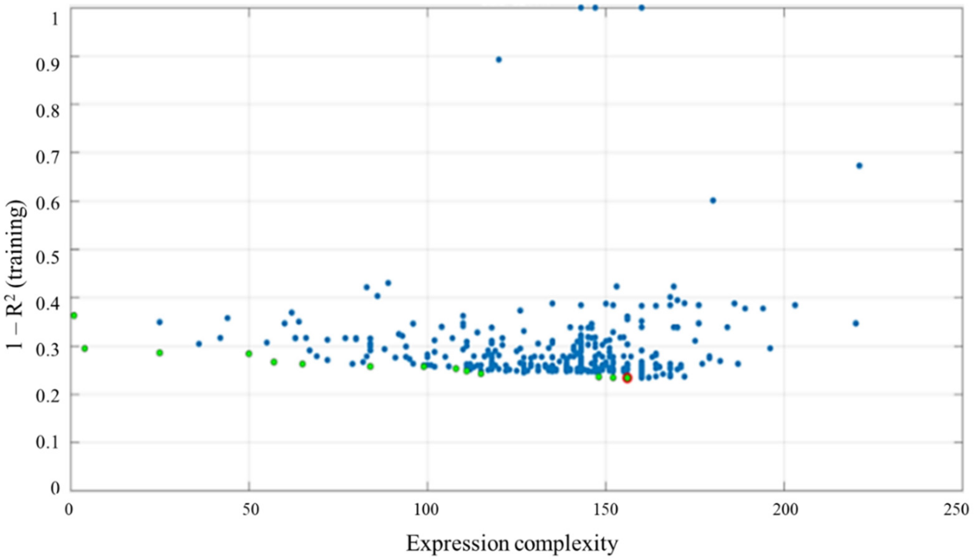
Figure 8 shows the accuracy versus the complexity of the developed models through a Pareto chart. There, the models with good performance are shown to be far less complex, as seen in the green dots in the Pareto chart. The red circle in Figure 8 for MGGP designates the best model described in this study, which is not outperformed by any other model regarding its simplicity and fitness. Thus, the equation of the MGGP model is the least complex and best fitted model out of the 1500 developed. From the Pareto front (Figure 8), developers can decide whether the incremental gain in performance is worth the related model complexity. The MGGP concept considers the analysis of multiple models, offering a superior number of alternatives to the stakeholder. A single model can also be chosen according to specific application constraints or demands.
According to the coefficients of Equations (1) and (2), as well as the variable importance in RF, the most important parameter in concrete carbonation is the concentration of carbon dioxide [23]. In fact, the literature indicates that the concrete carbonation rate fundamentally depends on the CO2 diffusivity, which, besides depending on the concrete’s porous structure and on its subsequent filling by other substances, particularly water, depends on the CO2 gradient from the concrete surface to carbonation front [23].
Performance indicators of the developed models, obtained from the testing samples, are shown in Table 4. The computational time to build the Model Tree (MT) is 0.08 s and 0.01 s to test the model, for Multi-Gene Genetic Programming (MGGP), the computational time is 14 min and 88 s, while for Random Forest (RF) the computational time is 40.5104 s. The performances of MT and RF are on par with the excellent performance of r = 0.953 and r = 0.955, respectively. MGGP, with r = 0.936, is close to, but below, the accuracy displayed by MT and RF, presenting simultaneously higher RMSE and MSE values. All these new models present lower RMSE values than those proposed in [11], developed using ANN and GP techniques. The former were developed with the purpose of overcoming the issue of having to consider two models when using the MLR technique, as in [23], due to the non-monotonic influence of RH in carbonation, as explained before. However, this use of two models, with RH playing the role of the splitting criterion, may be faced as a particular Model Tree. Thus, the performance indicators for the ensemble of the two MLR models proposed in [23] were computed, delivering values of r = 0.867, RMSE = 7.344 and MAE = 4.904. Therefore, MT, RF and MGGP models constitute an improvement concerning concrete carbonation coefficient prediction.
The scatter plot for MT, RF and MGGP models in Figure 9, Figure 10 and Figure 11 show a balanced scatter with no obvious under or over-prediction.
Furthermore, the performance of the model developed using MGGP, MT and RF were compared with the model developed using Artificial Neural Networks, Genetic Programming and Multiple Linear Regression [11]. Table 4 and Table 5 allow the comparison of the performance of the models, revealing that tree-based models display greater performance as compared to ANNs, GP and MLR.
Standard Random Forest (SRF) is a powerful method for high-dimensional regression and classification. For Random Forest, SRF gives an accurate approximation of the conditional mean of a response variable, revealing that RF provides information about the full conditional distribution of the response variable, not only about the conditional mean. Further conditional quantiles can be inferred with quantile regression forests (QRF)—a generalisation of random forests. Thus, quantile regression forests give a non-parametric and accurate way of estimating conditional quantiles for high-dimensional predictor variables that can be further studied for better predictions and accuracy [43,44]. The Gaussian Process Regression (GPR) can also be used, which is formulated in the Bayesian context. Specifically, the outputs of the GPR are assumed with a Gaussian process (GP) characterised prior by a mean function and covariance function. The adoption of sparse Gaussian process regression (GPR) allows the improvement of the short-term and long-term forecasting accuracy [45].
5. Conclusions
The present investigation constitutes a first approach towards modelling concrete carbonation using three data-driven techniques: Model Tree (MT), Random Forest (RF) and Multigene Genetic Programming (MGGP). Three models to predict concrete carbonation coefficient were developed and analysed, using MT, RF and MGGP. The performance of these models was compared with assembled MLR models, ANNs and GP models, which were previously applied in this field. In the different models proposed, MT, RF and MGGP have shown good performance in predicting the concrete carbonation coefficient. Further, these models revealed similar performance between them and an enhanced performance when compared with MLR, ANN and GP.
In all the models discussed, RF on average scores well on performance, as it leverages the power of multiple decision trees and it does not rely on the feature importance given by a single decision tree. MT coupled with the divide and conquer technique acquires the advantage of splitting until the lowest standard deviation error is reached and thus contributes to the good performance of models rather than a single tree. On the other hand, MGGP, with its evolution structure and operators such as reproduction, cross-over and mutation, offers the advantage of the selection of influential parameters deriving equations that lower the mean squared error. The weighted linear combination number of genes in MGGP helps to obtain better performance. Parameter influence in MT in the form of coefficients, permutation importance in RF, input frequency in MGGP and coefficients in MLR facilitate an understanding of the influential parameters, and thus we attempt to shatter the myth that these DDTs are “black boxes” and can be at least labelled as “grey boxes”.
This work also attempts to provide the readers with a tool in the form of series of equations that can be easily used through MT; while RF with series of trees can be combined further for easy deployment. MGGP presents a single equation that can be easily deployed and is user-friendly.
Author Contributions
Conceptualisation, A.S. and R.N.; methodology, S.L., P.K., P.D.; software, S.L., P.K., P.D.; validation, S.L., P.K., P.D.; formal analysis, A.S., R.N. and J.d.B.; writing—original draft preparation, S.L., P.K., P.D.; writing—review and editing, A.S., R.N. and J.d.B. All authors have read and agreed to the published version of the manuscript.
Funding
This research was funded by FCT (Portuguese Foundation for Science and Technology) through the project BestMaintenance-LowerRisks (PTDC/ECI-CON/29286/2017).
Institutional Review Board Statement
Not applicable.
Informed Consent Statement
Not applicable.
Data Availability Statement
The data presented in this study are available on request from the corresponding author.
Acknowledgments
The authors gratefully acknowledge the support of the Vishwakarma Institute of Information Technology (Pune, India) and to the CERIS Research Centre (Instituto Superior Técnico-University of Lisbon).
Conflicts of Interest
The authors declare no conflict of interest.
References
- Ciampoli, M. Time dependent reliability of structural systems subject to deterioration. Comput. Struct. 1998, 67, 29–35. [Google Scholar] [CrossRef]
- Ann, K.Y.; Pack, S.W.; Hwang, J.P.; Song, H.W.; Kim, S.H. Service life prediction of a concrete bridge structure subjected to carbonation. Constr. Build. Mater. 2010, 24, 1494–1501. [Google Scholar] [CrossRef]
- Huang, Q.; Jiang, Z.; Zhang, W.; Gu, X.; Dou, X. Numerical analysis of the effect of coarse aggregate distribution on concrete carbonation. Constr. Build. Mater. 2012, 37, 27–35. [Google Scholar] [CrossRef]
- Taffese, W.Z.; Al-Neshawy, F.; Sistonen, E.; Ferreira, M. Optimized neural network-based carbonation prediction model. In Proceedings of the International Symposium Non-Destructive Testing in Civil Engineering (NDT-CE) 2015, Berlin, Germany, 15–17 September 2015. [Google Scholar]
- Neville, A.M. Properties of Concrete, 4th ed.; Wiley: New York, NY, USA, 1996. [Google Scholar]
- Neves, R. The Air Permeability and Concrete Carbonation of Concrete in Structures. Ph.D. Thesis, Instituto Superior Técnico, Technical University of Lisbon, Lisbon, Portugal, 2012. [Google Scholar]
- Chang, C.F.; Chen, J.W. The experimental investigation of concrete carbonation depth. Cem. Concr. Res. 2006, 36, 1760–1767. [Google Scholar] [CrossRef]
- Monteiro, I.; Branco, F.A.; de Brito, J.; Neves, R. Statistical analysis of the carbonation coefficient in open air concrete structures. Constr. Build. Mater. 2012, 29, 263–269. [Google Scholar] [CrossRef]
- Papadakis, V.G.; Vayenas, C.G.; Fardis, M.N. Fundamental modelling and experimental investigation of concrete carbonation. ACI Mater. J. 1991, 88, 363–373. [Google Scholar]
- Kwon, S.J.; Song, H.W. Analysis of carbonation behavior in concrete using neural network algorithm and carbonation modeling. Cem. Concr. Res. 2010, 40, 119–127. [Google Scholar] [CrossRef]
- Londhe, S.N.; Kulkarni, P.S.; Dixit, P.R.; Silva, A.; Neves, R.; de Brito, J. Predicting carbonation coefficient using Artificial neural networks and genetic programming. J. Build. Eng. 2021, 39, 1022–1058. [Google Scholar] [CrossRef]
- Parthiban, T.; Ravi, R.; Parthiban, G.T.; Srinivasan, S.; Ramakrishnan, K.R.; Raghavan, M. Neural network analysis for corrosion of steel in concrete. Corros. Sci. 2005, 47, 625–1642. [Google Scholar] [CrossRef]
- Peng, J.; Li, Z.; Ma, B. Neural network analysis of chloride diffusion in concrete. J. Mater. Civ. Eng. 2002, 14, 327–333. [Google Scholar] [CrossRef]
- Kewalramani, M.A.; Gupta, R. Concrete compressive strength prediction using ultrasonic pulse velocity through artificial neural networks. Autom. Constr. 2006, 15, 374–379. [Google Scholar] [CrossRef]
- Bengio, Y. Learning deep architecture for AI. Found. Trends Mach. Learn. 2009, 2, 1–127. [Google Scholar] [CrossRef]
- Brusaferria, A.; Matteuccib, M.; Portolania, P.; Vitalia, A. Bayesian deep learning based method for probabilistic forecast of day-ahead electricity prices. Appl. Energy 2019, 250, 1158–1175. [Google Scholar] [CrossRef]
- Daou, H.; Raphael, W. A Bayesian regression framework for concrete creep prediction improvement: Application to Eurocode 2 model. Res. Eng. Struct. Mater. 2021, 7, 393–411. [Google Scholar] [CrossRef]
- Tesfamariam, S.; Martín-Pérez, B. Bayesian Belief Network to Assess Carbonation-Induced Corrosion in Reinforced Concrete. J. Mater. Civ. Eng. 2008, 20, 707–717. [Google Scholar] [CrossRef]
- Zewdu, W.T.; Sistonen, E.; Puttonen, J. Prediction of Concrete Carbonation Depth using Decision Trees. In Proceedings of the ESANN 2015 Proceedings, European Symposium on Artificial Neural Networks, Computational Intelligence and Machine Learning, Bruges, Belgium, 23–23 April 2015. [Google Scholar]
- Murad, Y.Z.; Tarawneh, B.K.; Ashteyat, A.M. Prediction model for concrete carbonation depth using gene expression programming. Comput. Concr. 2020, 26, 497–504. [Google Scholar]
- Londhe, S.N.; Kulkarni, P.S.; Dixit, P.R. A comparative study of concrete strength prediction using artificial neural network, multigene programming and model tree. Chall. J. Struct. Mech. 2019, 5, 1–42. [Google Scholar]
- Liu, P.; Wu, X.; Cheng, H.; Zheng, T. Prediction of compressive strength of High-Performance Concrete by Random Forest algorithm. IOP Conf. Ser. Earth Environ. Sci. 2020, 552, 012020. [Google Scholar]
- Silva, A.; Neves, R.; de Brito, J. Statistical modeling of carbonation in reinforced concrete. Cem. Concr. Compos. 2014, 50, 73–81. [Google Scholar] [CrossRef]
- Quinlan, J.R. Learning with Continuous Classes. In Proceedings AI”92; Adams, A., Sterling, L., Eds.; World Scientific: Singapore, 1992; pp. 343–348. [Google Scholar]
- Witten, I.H.; Frank, E. Data Mining: Practical Machine Learning Tools and Techniques with Java Implementations; Morgan Kaufmann: Los Altos, CA, USA, 2000. [Google Scholar]
- Granada, F.; Saroli, M.; de Marinis, G.; Gargano, R. Machine Learning Models for Spring Discharge Forecasting. Geofluids 2017, 2018, 8328167. [Google Scholar] [CrossRef] [Green Version]
- Breiman, L. Random Forests. Mach. Learn. 2001, 45, 5–32. [Google Scholar] [CrossRef] [Green Version]
- Tyralis, H.; Georgia, P.; Langousis, A. A brief review of random forests for water scientists and practitioners and their recent history in water resources. Water 2019, 11, 910. [Google Scholar] [CrossRef] [Green Version]
- Hai-Bang, L.; Tran, V.Q. Estimation of compressive strength of concrete containing manufactured sand by Random Forest. Int. J. Sci. Technol. Res. 2020, 9, 564–567. [Google Scholar]
- Londhe, S.N.; Dixit, P.R. Genetic programming: A novel computing approach in modeling water flows. In Genetic Programming—In New Approaches and Successful Applications; licensee InTech.16; IntechOpen: London, UK, 2012; Chapter 9. [Google Scholar]
- Searson, D.P.; Leahy, D.E.; Willis, M.J. GPTIPS: An Open-Source Genetic Programming Toolbox for Multigene Symbolic Regression. In Proceedings of the International Multi Conference of Engineers and Computer Scientists, Hong Kong, China, 17–19 March 2010. [Google Scholar]
- Searson, D.P.; Willis, M.J.; Montague, G.A. Co-evolution of non-linear PLS model components. J. Chemom. 2007, 2, 592–603. [Google Scholar] [CrossRef]
- Pandey, D.S.; Pan, I.; Das, S.; Leahy, J.J.; Kwapinski, W. Multi-gene genetic programming based predictive models for municipal solid waste gasification in a fluidized bed gasifier. Bioresour. Technol. 2015, 179, 524–533. [Google Scholar] [CrossRef] [PubMed] [Green Version]
- Hii, C.; Searson, D.P.; Willis, M.J. Evolving toxicity models using multigene symbolic regression and multiple objectives. Int. J. Mach. Learn. Comput. 2011, 1, 30–35. [Google Scholar] [CrossRef] [Green Version]
- Hair, J.F.; Black, W.C.; Babin, B.; Anderson, R.E.; Tatham, R.L. Multivariate Data Analysis, 6th ed.; Prentice-Hall Publishers: Englewood Cliffs, NJ, USA, 2007. [Google Scholar]
- Helene, P.R.L. Contribution to the Study of Corrosion of Concrete Reinforcement. Ph.D. Thesis, Polytechnic School, University of São Paulo, São Paulo, Brazil, 1993. (In Portuguese). [Google Scholar]
- Available online: https://waikato.github.io/weka-wiki/downloading_weka/ (accessed on 24 November 2021).
- Jain, A.; KumarJha, S.; Misra, S. Modeling and analysis of concrete slump using Artificial Neural Networks. J. Mater. Civ. Eng. 2008, 20, 628–633. [Google Scholar] [CrossRef]
- Legates, D.R.; McCabe, G.J., Jr. Evaluating the use of “goodness of fit” measures in hydrological and hydro climatic model validation. Water Resour. Res. 1991, 35, 233–241. [Google Scholar] [CrossRef]
- Londhe, S.N. Soft computing approach for real-time estimation of missing wave heights. Ocean. Eng. 2008, 35, 1080–1089. [Google Scholar] [CrossRef]
- Gandomia, A.H.; Mohammadzadeh, D.; Juan Luis Pérez-Ordóñez, S.B.; Alavid, A.H. Linear genetic programming for shear strength prediction of reinforced concrete beams without stirrups. Appl. Soft Comput. 2014, 19, 112–120. [Google Scholar] [CrossRef]
- Gandomi, A.H.; Atefi, E. Software review: The GPTIPS platform. Genet. Program. Evolvable Mach. 2020, 21, 273–280. [Google Scholar] [CrossRef] [Green Version]
- Dang, S.; Peng, L.; Zhao, J.; Li, J.; Kong, Z. A Quantile Regression Random Forest-Based Short-Term Load Probabilistic Forecasting Method. Energies 2022, 15, 663. [Google Scholar] [CrossRef]
- Meinshausen, N. Quantile Regression Forests. J. Mach. Learn. Res. 2006, 7, 983–999. [Google Scholar]
- Wang, H.; Zhang, Y.-M.; Mao, J.-X. Sparse Gaussian process regression for multi-step ahead forecasting of wind gusts combining numerical weather predictions and on-site measurements. J. Wind Eng. Ind. Aerodyn. 2022, 220, 104873. [Google Scholar] [CrossRef]
Figure 1.
An example of a typical Model Tree (adapted from [26]).
Figure 1.
An example of a typical Model Tree (adapted from [26]).

Figure 2.
Typical Random Forest tree (adapted from [26]).
Figure 2.
Typical Random Forest tree (adapted from [26]).


Figure 3.
Illustration of a Multi-Gene model (adapted from [26]).
Figure 3.
Illustration of a Multi-Gene model (adapted from [26]).

Figure 4.
Model for MT approach.

Figure 5.
Permutation importance of RF model parameters.

Figure 6.
Expressional tree for MGGP approach.

Figure 7.
Input frequency of MGGP model parameters.

Figure 8.
Pareto chart for MGGP model.

Figure 9.
Scatter plot and hydrograph for MT model.

Figure 10.
Scatter plot and hydrograph for RF model.

Figure 11.
Scatter plot and hydrograph for MGGP model.


Table 1.
Details of the data used for model development.
| Parameters | Min | Max | Mean | Mode |
|---|---|---|---|---|
| Clinker (kg/m3)—CC | 66.000 | 529.150 | 292.196 | 362.990 |
| Clinker/binder ratio (%)—CR | 20.000 | 100.000 | 80.228 | 95 |
| 28-day compressive strength in MPa—fc | 8.800 | 127.500 | 48.823 | 37.000 |
| CO2 content—CO | 0.020 | 50.000 | 15.490 | 0.040 |
| Number of curing days—d | 7 | 91 | - | 28 |
| Water/binder ratio—w/b | 0.240 | 1.000 | 0.501 | 0.370 |
| Relative humidity (%)—RH | 50 | 90 | - | 65 |
| Exposure class—X | 1 | 3 | - | 1 |
| Carbonation coefficient in (mm/year0.5)—k | 0.180 | 60.420 | 14.585 | 1.730 |
Table 2.
Parameter setting for MGGP.
| MGGP Parameters | Parameter Settings |
|---|---|
| Population size | 500–900 |
| Number of generations | 200–500 |
| Selection method | Tournament |
| Tournament size | 13–15 |
| Cross-over rate | 0.78–0.84 |
| Mutation rate | 0.14–0.20 |
| Termination criteria | 500 generation or fitness value less than 0.00 whichever is earlier. |
| Maximum number of genes and tree depth | 4–5 |
| Mathematical operations | +, −, ×, /, sin, cos, exp, √, {} |
Table 3.
Equations and weights for each gene.
| Term | Value | Weight |
|---|---|---|
| Bias | 9.83 | 9.83 |
| Gene 1 | −0.138 | |
| Gene 2 | 451 | |
| Gene 3 | 83,300 | |
| Gene 4 | 4.39 |
Table 4.
Performance indicators of the developed models.
| MT | RF | MGGP | |
|---|---|---|---|
| Time required for modelling | Building the model: 0.08 s Testing the models: 0.01 s | 40.5104 s | 14 min 88 s |
| r | 0.953 | 0.955 | 0.936 |
| RMSE | 3.871 | 3.584 | 4.453 |
| MAE | 2.341 | 2.032 | 2.546 |
Table 5.
Performance of models developed using ANNs, GP and MLR.
| Artificial Neural Network (ANNs) | Genetic Programming (GP) | Multiple Linear Regression (MLR) | |
|---|---|---|---|
| Correlation coefficient—r | 0.940 | 0.937 | 0.917 |
| Root mean square error—RMSE | 4.554 | 4.510 | 5.019 |
| Mean Absolute Error | 2.991 | 2.598 | 3.371 |
Publisher’s Note: MDPI stays neutral with regard to jurisdictional claims in published maps and institutional affiliations. |
© 2022 by the authors. Licensee MDPI, Basel, Switzerland. This article is an open access article distributed under the terms and conditions of the Creative Commons Attribution (CC BY) license (https://creativecommons.org/licenses/by/4.0/).
Share and Cite
MDPI and ACS Style
Londhe, S.; Kulkarni, P.; Dixit, P.; Silva, A.; Neves, R.; de Brito, J. Tree Based Approaches for Predicting Concrete Carbonation Coefficient. Appl. Sci. 2022, 12, 3874. https://doi.org/10.3390/app12083874
AMA Style
Londhe S, Kulkarni P, Dixit P, Silva A, Neves R, de Brito J. Tree Based Approaches for Predicting Concrete Carbonation Coefficient. Applied Sciences. 2022; 12(8):3874. https://doi.org/10.3390/app12083874
Chicago/Turabian StyleLondhe, Shreenivas, Preeti Kulkarni, Pradnya Dixit, Ana Silva, Rui Neves, and Jorge de Brito. 2022. "Tree Based Approaches for Predicting Concrete Carbonation Coefficient" Applied Sciences 12, no. 8: 3874. https://doi.org/10.3390/app12083874
Note that from the first issue of 2016, this journal uses article numbers instead of page numbers. See further details here.