
Immune System Programming: A Machine Learning Approach Based on Artificial Immune Systems Enhanced by Local Search


1
College of Engineering and Technology, American University of the Middle East, Egaila 54200, Kuwait
2
Department of Mathematics, Faculty of Science, Assiut University, Assiut 71516, Egypt
3
Department of Computer Science, Faculty of Computers & Information, Assiut University, Assiut 71526, Egypt
*
Author to whom correspondence should be addressed.
Electronics 2022, 11(7), 982; https://doi.org/10.3390/electronics11070982
Submission received: 15 February 2022
/
Revised: 15 March 2022
/
Accepted: 17 March 2022
/
Published: 22 March 2022
(This article belongs to the Special Issue Advances in Intelligent Systems and Networks)
Abstract
:The foundation of machine learning is to enable computers to automatically solve certain problems. One of the main tools for achieving this goal is genetic programming (GP), which was developed from the genetic algorithm to expand its scope in machine learning. Although many studies have been conducted on GP, there are many questions about the disruption effect of the main GP breeding operators, i.e., crossover and mutation. Moreover, this method often suffers from high computational costs when implemented in some complex applications. This paper presents the meta-heuristics programming framework to create new practical machine learning tools alternative to the GP method. Furthermore, the immune system programming with local search (ISPLS) algorithm is composed from the proposed framework to enhance the classical artificial immune system algorithm with the tree data structure to deal with machine learning applications. The ISPLS method uses a set of breeding procedures over a tree space with gradual changes in order to surmount the defects of GP, especially the high disruptions of its basic operations. The efficiency of the proposed ISPLS method was proven through several numerical experiments, including promising results for symbolic regression, 6-bit multiplexer and 3-bit even-parity problems.
1. Introduction
A genetic algorithm (GA) is a meta-heuristic search algorithm that mimics the biological processes of natural selection and survival of the best. GA has been studied and experimented with widely through many applications in several areas [1]. Next, genetic programming (GP) was introduced as a new evolutionary algorithm that inherits the GA strategy [2,3]. The first appearance of pure GP was written in 1985 by Nichael Cramer [4]. He used the idea of GA to propose the tree-based genetic programming approach. Then, this work became popularized via a search technique created by John Koza in the 1990s [5,6]. John Koza demonstrated the feasibility of the GP in many application areas. Since then, the number of research in this field has spread and increased rapidly, and the concept of GP was widely applied in plenty of applications, such as classification [7,8], control [9,10], dynamic processes [11,12], electrical circuit design [13,14], chemical engineering including polymer design [15,16], regression [17,18], and signal processing [19,20].
The main differences between GA and GP can be summarized in the representation of solutions and application fields. Candidate solutions in GP are represented as executed forms, usually hierarchical tree forms, while solutions in GA are represented as fixed-length binary strings or linear real-valued codes [16]. In GP, each tree consists of a set of leaf nodes called terminals and a set of internal nodes called functions. The functions and terminals are defined to represent candidate solutions depending on the problem under study. Moreover, the tree-based representation of a solution is an important feature of GP and enables it to handle and solve a variety of applications. The GP algorithm optimizes a population of computer programs in tree-based representation that evolve in each generation according to their fitness value defined by a program’s ability to solve the problem. The algorithm begins the search with a randomly generated set of computer programs. Then, based on their fitness, some individuals are selected from the current population to breed new individuals, using the crossover and/or mutation operators. This process is iterated to drive the population toward the main goal. Consequently, GP is known to pursue the goal of machine learning, which means that computers program themselves without humans guiding them step by step. In addition, many challenging real-world problems have been solved by using the GP technique [18,21]. Despite all these GP successes and applications, standard breeding operators can spoil promising solutions, and there are some risks that the optimal structure will be difficult to find. Therefore, there have been many attempts to modify GP operators with the purpose of maintaining promising individuals and reaching optimal solutions [13,22].
Meta-heuristics are often seen as promising options for solving problems that can be modeled or transformed into optimization problems. The most widely used data-structure types that are used in meta-heuristics are real-valued vectors and bit strings [23]. Choosing a suitable meta-heuristic method that solves a given problem is fundamental. The performance of different meta-heuristics varies, even when they are applied to the same problem. Moreover, the “No Free Lunch” theorem reports that the average performance of search algorithms is equal over all possible applications, so no search method is better than others in general [24]. The presence of a large variety of meta-heuristics methods has stimulated many attempts to extend the scope of meta-heuristics to deal with the tree-data structure and accommodate different types of applications. Using the tree-data structure, there are a limited number of successful attempts to produce alternatives to GP from traditional meta-heuristic methods, such as memetic programming [25], tabu programming [26], and scatter programming [27]. Therefore, we aim to extend more efficient meta-heuristics methods and design new machine learning tools that use tree data structure and manipulate computer programs.
This paper introduces the immune system programming with a local search (ISPLS) algorithm that searches for an appropriate computer program and inspires its idea from the artificial immune system (AIS) algorithm. The AIS algorithm is a meta-heuristic method that takes inspiration from the human natural immune system. The immune system has many attributes that would be advisable for an artificial system to have, such as self-organization, learning, adaptation, and recognition. AIS is growing rapidly, and it applies the principles of the natural immune system in a wide range of application areas [28,29]. Therefore, we introduce ISPLS as a new machine learning approach that behaves as an AIS algorithm but deals with computer programs that are represented as trees. The main contribution of the proposed algorithm is to plan more alternatives to the GP algorithm in order to adapt more application areas by using the evolutionary and adaptive mechanisms of AIS. The main focus is that ISPLS uses breeding operators over a tree space to generate new offspring from the current parent. These breeding operators make the effects of the program under some restrictions. In addition, ISPLS exploits the breeding operators in the structure of the local search (LS) procedure with gradual changes in order to overcome the defects of GP. The results show that ISPLS is promising in terms of solving many benchmark problems; symbolic regression, 6-bit multiplexer and 3-bit even-parity problems.
The paper is organized as follows. The next section illustrates the main framework of MHP. Section 3 describes the basic concept of AIS, which is an inspirational source for the proposed algorithm. Section 4 shows the proposed ISPLS algorithm together with breeding operators over tree space and the LS procedure that achieves the intensification principle in the most promising areas. The numerical results of the ISPLS method are shown in Section 5 for three types of benchmark problems: symbolic regression, 6-bit multiplexer, and 3-bit even-parity problems. Finally, the conclusion appears in Section 6.
2. Meta-Heuristic Programming (MHP)
Meta-heuristics can be categorized into two categories: population-based methods and point-to-point methods [1]. In the latter group of methods, at the end of each iteration, the search provides only one solution with which the search then begins in the next iteration. On the other hand, at the end of each iteration, population-based methods retrieve a set of many solutions. The most famous meta-heuristic method is the GA, which is considered an example of population-based meta-heuristics, while tabu search, simulated annealing and ant colony optimization are point-to-point meta-heuristics [30,31].
The MHP is a framework that attempts to cover many of the well-known meta-heuristic methods and generalizes the data structures used in these methods to be tree-data structures, instead of bit strings or vectors of numbers [26]. In the MHP framework, the initial computer programs can be adapted through four procedures to find an acceptable target solution to the problem at hand. The order of these procedures depends on the meta-heuristic algorithm. These procedures are as follows [26,30]:
- TrialProgram: attempts to generate trial programs from the current program(s).
- Enhancement: enhances the search process by exploiting the best region (good regions are explored more thoroughly to find better solutions) or escaping from the local region if an improvement step is not achieved.
- UpdateProgram: selects one or more programs to use for the next generation or the next iterate.
- Diversification: directs the search to new unexplored regions in the search space or to escape from the local area.
TrialProgram and UpdateProgram procedures are the basic procedures in MHP. The other procedures are added to achieve better and faster performance from MHP. In fact, by using these procedures, the MHP behaves as an intelligent hybrid framework [30]. The layout of the MHP framework follows the following steps:
- 1.
- Initialization: Generate an initial population (or an initial program ) and initialize the iteration counter .
- 2.
- Main Loop: Repeat the main search steps (2.1)–(2.4) for M times.
- 2.1
- Trial Solutions: Use TrialProgram Procedure in order to create trial programs from the current ones (or ).
- 2.2
- Enhancement: Apply Enhancement Procedure to improve the programs in .
- 2.3
- Solution Updating: Apply UpdateProgram Procedure to choose the next population (or next iterate program ).
- 2.4
- Update Parameter: Update the current parameters.
- 3.
- Termination: Proceed to Step 5 if the termination criteria are met.
- 4.
- Diversification: If it is necessary to diversify, apply DiverseProgram Procedure to update the population (or solution ) with new diverse solutions. Set and go to Step 2.
- 5.
- Intensification: Apply Enhancement Procedure to improve the best programs obtained so far.
3. Artificial Immune System
The immune system of each organism differs according to its attributes. The human immune system aims to protect the human body from harmful bacteria, fungi, parasites, and viruses that are classified as pathogenic sources and capable of causing disease [32]. Moreover, the immune system recognizes pathogens through antigen molecules and presents different forms of antibodies consisting of T cells and B cells to generate a reaction against these pathogens [33,34].
Although diseases come in many forms, the immune system is considered an adaptive and robust system because it is capable of forming a group of immune cells of many shapes and sizes [35]. These cells combine to form more complex structures called antibodies. In order for the immune system to be more effective, it can change the structure of immune cells to maximize their affinity for the antigen through the process of affinity mutation. Thus, despite the complexity of diseases, immune cells try to adapt themselves to fight these diseases without any prior knowledge of their structure [36,37].
Clonal selection is a popularly accepted theory used to model the immune system’s responses to infection. The clonal selection was proposed by Frank Burnet in 1959 [38]. It is based on the cloning and affinity maturation concept. The entire process of clonal selection is based on antigen recognition and cell proliferation. B cells are used to destroy all antigens that invade the body. When the body is exposed to a foreign antigen attack, these B cells clone a specific type of antibody, , which achieves the best bond with antigen . The bending between and is measured by how well the paratope matches an epitope of the . A closer match means a stronger bond. The mutation process is applied to the cloned cells to ensure diversity. Moreover, the selection process ensures that the cells with a higher affinity survive [32].
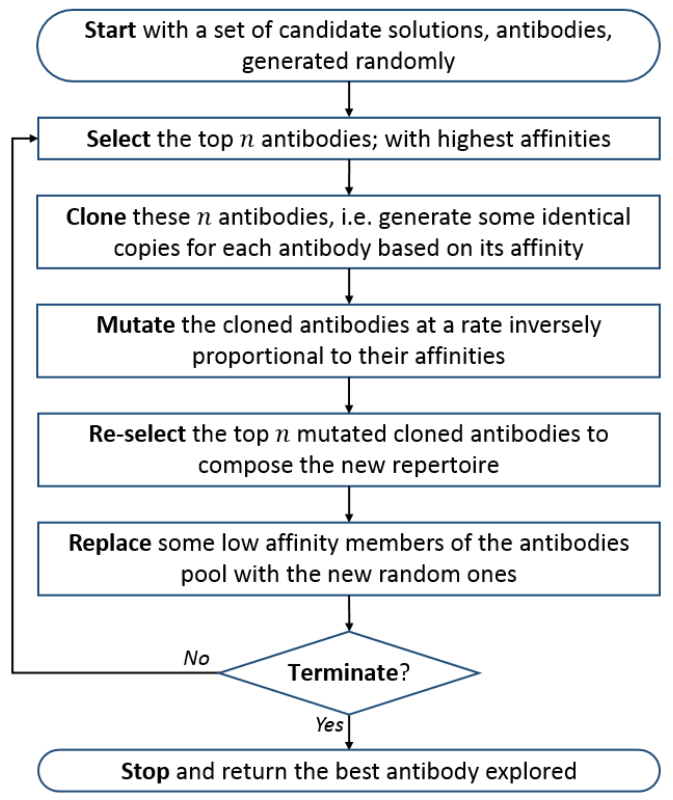
Many artificial immune algorithms have been proposed to imitate the clonal selection theory. De Castro and Von Zuben [32] introduced a clonal selection algorithm called CLONALG to solve learning and optimization problems in 2002. The CLONALG algorithm is illustrated in Algorithm 1, and its flowchart is explained in Figure 1. For more details, see [32].
| Algorithm 1 CLONALG algorithm. |
|
From the CLONALG algorithm, one can note that individuals have independent mutation rates based on their affinities. Specifically, promising solutions that are close to the optimal solution are processed with smaller mutation rates, while those that fall far from the optimal solution undergo greater mutation rates [32]. The cloning process means reproducing new solutions that are copies of their parents. The number of clones, , generated from each of the n best solutions is calculated as follows:
where is a clonal factor , i is the current solution rank , and is the population size; see [37]. By observing the AIS algorithm, one can note that the clonal selection immune algorithm is a class of evolutionary algorithms and that it is inspired by the human immune system [31].
4. Immune System Programming with Local Search
The proposed ISPLS algorithm deals with a computer program that is represented as a tree with some inner nodes acting as functions and some external nodes representing terminals. The set of functions and the set of terminals and their domains are determined by the user based on the problem at hand. In addition, the tree construction is converted into executable code during the coding process. The search space in the case of the ISPLS algorithm is the collection of all computer programs that can be represented as tree forms. In addition, each computer program has some neighborhoods that should be generated by using the breeding operators that are illustrated in Section 4.1. With these breeding operators, the LS procedure is defined in Section 4.2 for creating new computer programs that meet certain conditions, which are explained later. Section 4.3 summarizes the full steps of the proposed ISPLS algorithm.
The running algorithm of ISPLS achieves the MHP conditions as shown in the following stages:
- Initial Stage: The set of initial programs is randomly generated.
- Evaluation Stage: For each program in , evaluate its efficiency through its ability to solve the considered problem.
- Clonal Stage: Create some clones of the most promising programs in and save them as the set.
- Mutation Stage: Apply a mutation mechanism on programs in the set to create a new set of children programs called the set.
- Divers Stage: Construct a new set, named the set, that contains diverse programs to assist the search process variety.
- Replace Stage: Replace the set with selected programs from .
By iterating the last five stages, the ISPLS looks through the search space of the computer program to gain access to an elite program that solves the problem under consideration. However, during the search process of the main algorithm, the ISPLS should achieve the balance between the intensification search and the diversification search. In fact, the intensification search is achieved by ISPLS through the clonal process and uses the mutation process on a small scale to get close to the neighboring of the current program. The diversification search can be done by carrying out a large-scale mutation process of some selected programs, as long as a new set of random programs is generated in each generation during the diversification stage.
In the clonal stage, the fitness values of all programs in the current population are used to rank these programs in descending sort order. Then, each of the first n programs is replicated several times to produce clones according to Equation (1). On the other hand, the ISPLS algorithm implements a mutation process with different scales of each program in the first n best programs using a factor called , which is calculated as follows:
where is a given parameter with a positive value, and i is the program rank; see [37]. The values of and are proportional to the program efficiency. For the best program in the current population, arrives at its maximum value, and reaches its minimum value. Therefore, the algorithm applies several mutations with small scales and produces a deep exploration around the best program. As long as i increases, decreases, and increases. Therefore, the algorithm applies mutation processes using a large scale to defeat the trapping in the local maxima or minima.
4.1. Breeding Operations
The mutation stage has a main role in advance of the search operation. The ISPLS algorithm depends on the LS procedure to perform the mutation process and obtain good programs in the neighborhood of the current one. The LS procedure employs three types of breeding operations, shaking, grafting, and pruning, in different scales to achieve harmony between intensification and diversification searches. The basic ideas of these breeding operations are taken from the tabu programming [26], with some modifications. Those three operations can be classified into two categories: fixed-structure search and dynamic-structure search. Fixed-structure search discovers the neighborhood of the present program by altering its nodes without changing its structure. On the other hand, the dynamic structure search is able to modify the structure of the current program through extending some of its terminal nodes or deleting some of its subtrees. The LS procedure uses the process as a fixed structure search. However, and are employed as dynamic-structure searches. Before starting the description of shaking, grafting and pruning procedures, some basic notations are defined. For a program P, we define the following:
- , the program depth, is the number of links in the path from the root of the program P to its farthest terminal node.
- is the number of links in the path from node l to the root of the program that contains l.
- is the maximum depth for a program that is allowed during the search process.
- is the number of all nodes in the program P.
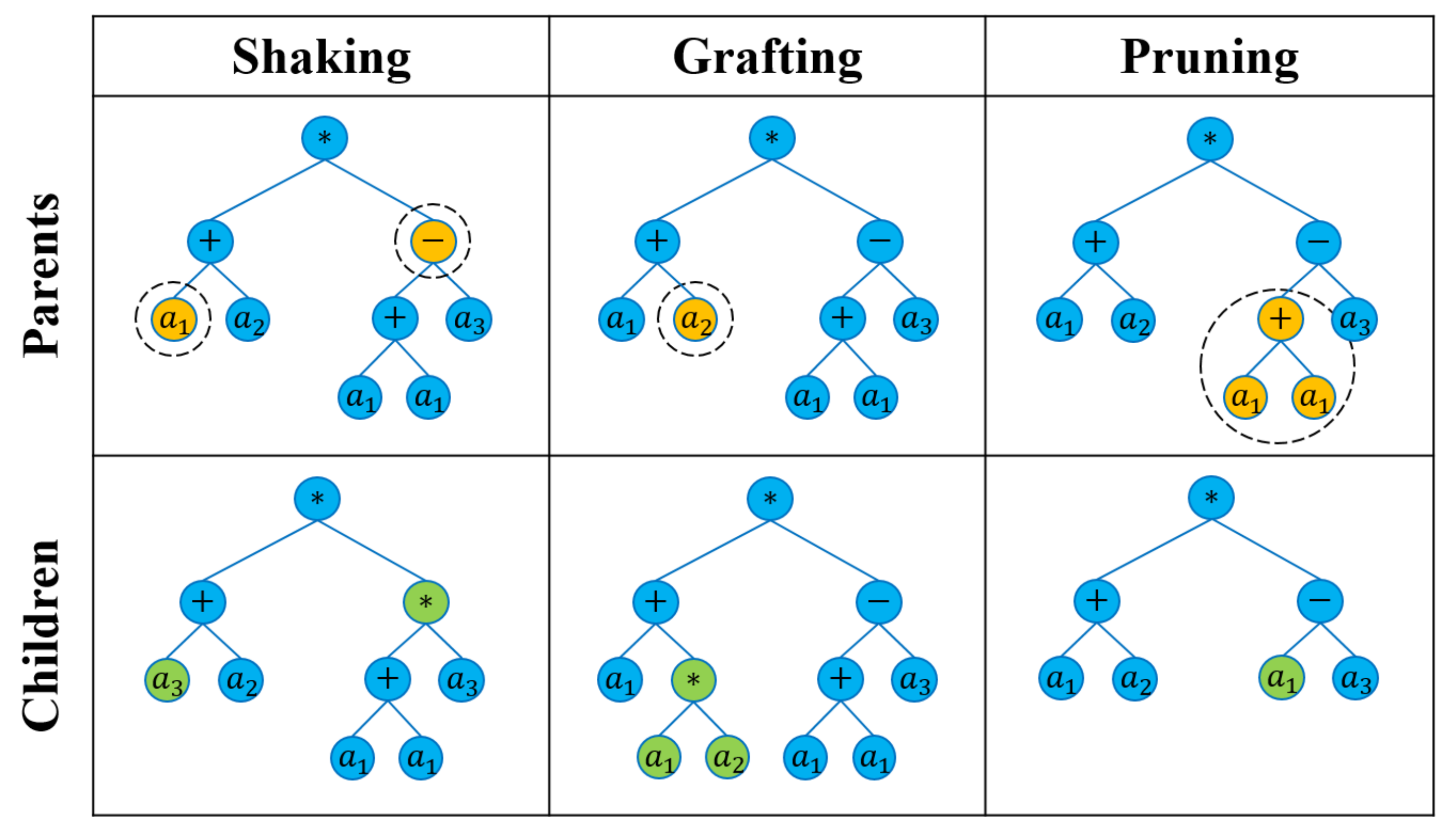
4.1.1. Shaking Procedure
The shaking search process can be classified as a fixed-structure search. It creates a new set of computer programs called from the current program P by changing, at most, nodes that are selected randomly from P without any effect on the structure. The selected nodes and their alternatives should have the same properties, i.e., a terminal node is replaced with a new terminal one, and a function node is replaced with a new function on conditions that have the same number of arguments. Procedure 1 introduces the description of the shaking process that creates a set of N trials from the current program P, with a maximum number of changes for each trial.
Procedure 1.
- 1.
- Initialization: Set Γ to hold the numbers of all changeable nodes in P and set the program pool to be empty.
- 2.
- If Γ is empty, then terminate. Otherwise, let equal to .
- 3.
- Main Loop: For , do the following Steps 3.1–3.4.
- 3.1
- Set .
- 3.2
- Let v be a random permutation of numbers in Γ.
- 3.3
- For , do the following Step 3.3.1.
- 3.3.1
- If a similar alternative value from the collection of terminals or functions exists, replace with it.
- 3.4
- Add to .
- 4.
- Return with .
It is important to note that in Step 3.3.1 of Procedure 1, a leaf node is exchanged with another leaf node from the terminal set, and a function node is exchanged with another function node of the same number of arguments. However, the procedure is terminated if there are no alternatives for all nodes in the program.
4.1.2. Grafting Procedure
The grafting search is performed as a dynamic structure search to enhance the search process. This process creates a set of new programs altered from a program P through the expansion of some of its terminal nodes, which are selected randomly, to be subtrees. Procedure 2 introduces the grafting process to create N trial programs from a program P, where at most terminals are expanded to become subtrees.
Procedure 2.
- 1.
- Initialization: Initialize to be an empty program pool set.
- 2.
- Main Loop: For , do the following Steps 2.1–2.3.
- 2.1
- Set .
- 2.2
- For , do the following Steps 2.2.1–2.2.3.
- 2.2.1
- Set T to contain all terminal nodes in whose depth is less than or equal to .
- 2.2.2
- If T is empty, then terminate. If not, choose a terminal node at random.
- 2.2.3
- The node t is replaced with a new randomly generated subtree with depth i.
- 2.3
- Update and add it to .
- 3.
- Return with .
4.1.3. Pruning Procedure
The pruning search process is also another type of dynamic structure search, and it is considered the reverse of the grafting process. The pruning process generates a new set of changed programs from the program P by changing some of its branches by some terminals. Procedure 3 illustrate the description of the pruning process to create N trials from the program P, where the procedure cuts, at most, branches of a specified depth, selected randomly, for each trial.
Procedure 3.
- 1.
- Initialization: Initialize to be an empty program pool set and update N to be equal to .
- 2.
- Main Loop: For , do the following Steps 2.1–2.3.
- 2.1
- Set .
- 2.2
- For , do the following Steps 2.2.1–2.2.3.
- 2.2.1
- Set S to contain all subtrees in whose depth is equal to i.
- 2.2.2
- From S, choose a subtree θ at random.
- 2.2.3
- Replace θ with a terminal node chosen from the set of terminals at random.
- 2.3
- Update and add it to .
- 3.
- Return with .
Figure 2 shows, graphically, the strategy of the three types of breeding operations. As was mentioned above in the breeding operators, some values must be determined before calling these three procedures, such as N and . The N value determines the number of trials that are produced, but also this number of trials is dependent on the number of functions and terminals in the original solution. On the other hand, the value controls the amount of changes in each trial; with more detail, if the value of and , that means the shaking procedure is introduced in three trials. The first trial is generated by choosing a random node and replacing it with another alternative node, and the second trial is also generated by choosing one random node and replacing it with an alternative node, and so on. On the other hand, when the grafting procedure is called, the first trial is generated by choosing a random node and replacing it with a subtree of depth equal to 1, while the second trial is generated by choosing a random node and replacing it with a subtree of depth equal to 2, and so on.
Applying the breeding operators’ procedures and getting on the neighbors of the current solution P requires a lot of information about it, such as the size of P, the number of terminal nodes and function node in P, the number of the argument to each function node in P, and the depth of each branch in the solution. Moreover, by applying the previous breeding procedures, no one asserts obtaining all the neighbors around an original solution. So, these procedures are considered stochastic search procedures that obtain random candidate solutions in the neighborhood of the solution at hand. In other words, you can obtain totally different results in each call of any of these procedures, although you are using the same solution and the same parameters.
To enhance the result of the search process, the previous breeding procedures were designed to be able to explore the search space gradually. They can be applied with a small scale of changes to avoid the disruption of the current solution and also applied with a big scale of changes to keep the principle of diversity. The gradual changes keep the balance between the intensification and the diversification principles in the search process, and this is considered a major issue that should be taken into account in designing efficient search procedures [1]. On the other hand, the ISPLS is using an LS procedure that is a strategy that exploits the previous breeding procedures to improve the search process. The next subsection illustrates the LS procedure with its details.
4.2. LS Procedure
In this subsection, the breeding procedures that were shown in Section 4.1 are employed in the LS procedure to create new programs under some restrictions. Specifically, when intensification is desired, the LS procedure is used on a small scale. Exactly the contrary, the LS procedure is used on a large scale when the diversification search is required. The LS procedure is proposed to find the best program in the neighborhood of the current program and also to cover all the search space by moving from one area to another. Procedure 4 illustrates the steps of the LS procedure, where the main loop of the procedure is terminated if the maximum number of non-improvements is reached.
Procedure 4.
- 1.
- Initialization: Set , and .
- 2.
- Main Loop: do the following Steps 2.1–2.5 while .
- 2.1
- Apply the shaking procedure and set X = Shaking().
- 2.2
- Set be the best program in X.
- 2.3
- If is better than P, then set and go to Step 2.1. Otherwise, set .
- 2.4
- If P is better than , then set = P.
- 2.5
- If , apply only one option randomly selected from the following choices (i) or (ii).
- (i)
- Apply the grafting procedure and set Y = Grafting().
- (ii)
- Apply the pruning procedure and set Y = Pruning().
Let , where is the best program in the Y.
- 3.
- Termination: Return .
In the initialization step, Step 1, the procedure starts with a program P that is received from another algorithm. In addition, and a counter k take their initial values. The counter k is used to count the number of non-improvements during the search process. The user must determine two positive integers, and N. Specifically, is the maximum number of non-improvements, and N represents the number of trial programs that are generated in the neighborhood of the current program by using shaking, grafting and pruning search procedures. In Step 2.1, an inner loop iterates the shaking procedure until it finds a better program near P. Then, it replaces the current program P, and the procedure goes back to Step 2.1. Otherwise, the LS procedure updates the counter k and proceeds to Step 2.4 to update if a better program is explored. In Step 2.5, when the number of non-improvements reaches the maximum number of non-improvements , the procedure stops and returns with . Otherwise, it proceeds to Step 2.6 to diversify the search process by applying either the grafting or the pruning procedure, which is chosen randomly. In Step 2.7, the procedure replaces P with the best program in Y and updates if a better program is explored, then goes back to Step 2.1. Finally, when the termination condition is satisfied, the algorithm stops at Step 3 and returns with the best program found. The main loop is repeated as long as the value of the counter k does not exceed the maximum value . Therefore, the number of fitness evaluations needed during a single run of the LS procedure varies depending on the improvement of the current program. Figure 3 shows the flowchart of the proposed LS procedure.
As mentioned above, the strategy of the LS procedure depends on the shaking procedure that detects the close tree structures around the current program and moves to the best of them. Applying this operation several times leads to making good exploration around the current program; the strategy also uses the dynamic structure search to move to another area when the change for the better is stopped in this region. Therefore, the ISPLS algorithm exploits the LS procedure to enhance the search operation.
4.3. ISPLS Algorithm
Algorithm 2 summarizes the complete steps of the ISPLS method, using the breeding operations and procedures introduced in the previous subsections, where is given, and it represents the rate of the most promising solutions that will be cloned and mutated. Additionally, the value is given, and it represents the rate of new programs that are created in the diversification stage.
The termination condition is satisfied by one or more of the following: the algorithm reaches the maximum number of iterations, the algorithm reaches the maximum number of fitness evaluations, or the algorithm obtains the optimal solution.
| Algorithm 2 ISPLS algorithm. |
|
The ISPLS algorithm uses the strategy of the artificial immune system and provides it by the LS procedure to guide the search to an optimal solution in a suitable time. In Steps 1.1–1.3, the algorithm begins by reading and determining the parameter values, and then it generates the initial solutions in a set. Then, it sorts the initial population in descending order according to the fitness value to give the good solutions more opportunity for improvement by the LS procedure. In each iteration, the algorithm selects the best solutions in the population and applies the LS procedure to each of them. The algorithm is designed to consider the number of trials of one solution that are represented by each of the breeding operators as the number of cloning of this solution to ensure that there is no repetition in the output of the breeding operators. In addition, each solution has a single substitute in the next generation. The algorithm in each generation enhances the search operation by adding a new set of solutions that is generated randomly to increase the diversification. The main loop is repeated until a termination condition is satisfied, then it returns with the best program obtained.
The set represents the memory section, while the other elements of the population are considered the remaining section. The replace stage rivals between the output of the LS procedure , the remaining section, and the newly generated solution .
The computational complexity of the worst-case scenario for a single iteration of the main loop of Algorithm 2 is , and it can be interpreted as follows:
- Step 2.1 is , to sorting all programs in .
- Step 2.2 is , to fill .
- Step 2.4 is , to update , where .
- Step 2.5 is , to generate a set of d programs for .
- Step 2.7 is , to update .
It means that the computational complexity of the proposed ISPLS algorithm, Algorithm 2, is , where represents the maximum number of iterations. Similarly, the computational complexity of the AIS algorithm is , since AIS uses a simple mutation procedure to update [35]. As a result, the complexity of ISPLS is higher than the corresponding complexity of AIS, unless the LS procedure succeeds in improving the programs in and finds the optimal solution.
5. Experimental Results
In this section, we focus on the performance of the proposed ISPLS algorithm under different environments. In all experiments, the algorithm is terminated as soon as the maximum number of fitness evaluations is reached or the optimal solution is found. In addition, some comparisons between the ISPLS algorithm and other algorithms are reported. It is important to note that, for the ISPLS algorithm, the initial population in each test problem is generated as full trees of depth , which can be considered a parameter.
5.1. Test Problems
5.1.1. Symbolic Regression Problems
The main target in a symbolic regression problem is to find a mathematical formula that fits a given data set. The fitness value for a program is computed as the sum with an inverse sign of absolute errors between the expected output and the actual output of all fitness cases. Therefore, the maximum fitness value for this problem is 0. In this paper, we considered four symbolic regression problems where a polynomial function f will be given, and the target for each problem is to produce a new function g that approximates the original polynomial with the minimum error by using a data set generated in random from f [26]. The set is used as the function set for all symbolic regression problems, where the operator % is the protected division, i.e., if and otherwise [30,39].
The Fourth Degree Polynomial
In this subsection, we consider the quartic polynomial function , where a data set of 20 fitness cases of the form is obtained by choosing x uniformly at random in the interval [−1, 1] [2,26]. This problem is referred to as the SR-QP problem in this paper. The function set of the SR-QP problem is and the terminal set is the singleton .
The Quintic Degree Polynomial
In this problem, we consider the quintic polynomial function , where a data set of 50 fitness cases of the form is obtained by choosing x uniformly at random in the interval [−1, 1] [39]. This problem is referred to as the SR-QUP problem. The function set of the SR-QUP problem is set to be and the terminal set is .
The Sixtic Degree Polynomial
Here, we consider the sixtic polynomial function , where a data set containing 50 fitness cases of the form is obtained by choosing x uniformly at random in the interval [−1, 1] [39]. This problem is referred to as the SR-SP problem throughout the remainder of this paper. Moreover, we use as the function set for the SR-SP problem and the terminal set is .
The Multivariate Polynomial
In this problem, the multivariate polynomial function = is considered, where a data set of 50 fitness cases of the form (,) is generated randomly with This problem is referred to as the POLY-4 problem in this paper. Similarly, to the previous problems, we use as the function set; however, the variables and are used to form the terminal set for the POLY-4 problem.
5.1.2. 6-Bit Multiplexer Problem
The input to the Boolean 6-Bit Multiplexer (6-BM) function is composed of two “address” bits and , and four “data” bits and . However, the value of the 6-BM function is the data bit that is singled out by the two address bits, and All combinations of the arguments are considered fitness cases. The truth table is formed by calculating the Boolean value of each combination. The fitness value of a program is evaluated as the number of fitness cases, where the Boolean values returned by that program are the correct Boolean values. Therefore, the program’s maximum fitness value is the same as the number of fitness cases, which is 64 [26,30]. For the 6-BM problem, the function set is the set of Boolean functions where returns y if x is true, and it returns z otherwise. Moreover, the set of arguments is used as the terminal set.
5.1.3. 3-Bit Even-Parity Problem
A parity bit is a check bit (1 or 0) that is added to the end of a string of binary code. This parity bit is used to denote whether the total number of 1-bits in the string is even or odd. Parity bits are used for error detection purposes, e.g., detecting of transmission errors [40]. The Boolean 3-bit even-parity (3-BEP) function is a function of 3 arguments of bit type, namely and . Therefore, the function returns 1 if the arguments include an even number of 1-bits, and it returns 0 otherwise. All combinations of the arguments are considered fitness cases. The truth table is formed by calculating the Boolean value of each combination. The fitness value of a program is computed as the number of fitness cases, where Boolean values returned by the program are the correct Boolean values. Therefore, the program’s maximum fitness value for the 3-BEP problem is 8 [27,39]. For the 3-BEP problem, the set of Boolean functions forms the function set, and the set of arguments forms the terminal set [41].
5.2. Parameter Tuning
This subsection discusses the performance of the ISPLS algorithm through the benchmark problems in the previous subsection. We focus on the effect of the ISPLS parameters and their proper values for each test problem. Therefore, a set of different values is specified for each of these parameters. Then for each value, 100 independent runs are performed in order to calculate the mean value of the number of fitness evaluations used through these independent runs. Other parameters are fixed at their standard values given in Table 1. These values are determined from the common setting in the literature and from some pilot experiments as well. The results obtained from parameter tuning differ from one problem to another because of the difference in the problem’s structure and complexity. This is the reason for applying the parameter tuning process to each problem. Through all the experiments in this paper, we use the maximum depth , which means the maximum length of a program is 255 nodes for the SR-QP, SR-QUP, SR-SP, POLY-4 and 3-BEP problems. However, the maximum length as of a program for the 6-BM problem is 3280 since the function set contains the ternary function .
Table 2 and Table 3 show the performance of the ISPLS algorithm with different values of each parameter for all the problems under consideration. In all the experiments shown in these tables, the ISPLS algorithm terminates when it obtains the optimal program with the maximum fitness value.
We used the ANOVA statistical test to analyze the performance of the proposed algorithm using different parameter values for 6 benchmark problems with the full set of runs, 20,900 independent runs. All data were transformed using log function, then analysis of variance was performed using Proc Mixed of the SAS version 9.2, and mean values (per 100 runs) were compared by Duncan’s at a significance level of [42]. The results of the statistical analysis indicate that the benchmark problems are independent and the selection of parameter values is a problem-based issue. Similarly, the results indicate that the set of parameters have significant effect and independent for . The crucial parameters for the ISPLS algorithm are and . The best value for depends on the problem itself, and suitable values are limited between 3 and 5 for all problems under study. The value of should be large enough, but not too much, to cover the entire search space. For all problems, it is preferable to specify a value for between 25 and 75. Moreover, large values of reflect the best performance for all problems, and the best values of are limited from to . On the other hand, and have a moderate effect of the performance of the algorithm. Furthermore, the performance is stable for all proposed values of and . The computational results presented in Table 2 and Table 3 also reflect the same conclusions obtained from the statistical test of ISPLS parameter values.
5.3. Comparative Results
In this subsection, we examine the performance of the ISPLS algorithm along with some different GP algorithms that appeared in the literature.
5.3.1. ISPLS Algorithm vs. GPLab Toolbox and TP Algorithm
GPLab [43,44] is a Matlab toolbox that includes the traditional features and capabilities of GP tools that can be used for a wide range of uses. In this experiment, we compared the results of the ISPLS algorithm with the corresponding results of the GPLab toolbox, assuming that both have a limited number of fitness evaluations. Table 4 illustrates the comparison between ISPLS and GPLab, where is referred to as the maximum allowed number of fitness evaluations [26].
Tabu programming (TP) algorithm is an extended version of the tabu search algorithm [30], in which the search space of the TP algorithm is a collection of all computer programs that can be represented as trees. The main contribution of TP is designing other alternatives to the GP algorithm in order to accommodate more application areas. Table 4 illustrates the comparison between ISPLS, TP and GPLab for 100 independent runs with a limited number of fitness evaluations for each run. Specifically, the maximum number of fitness evaluations for each run is 2500 for the SR-QP problem and 25,000 for both 6-BM and 3-BEP problems [26]. The results of these algorithms are shown in Table 4 in terms of the mean of the number of fitness evaluations needed for each run and the success rate. A one-sample t-test, two-tailed, is used to compare the significant differences between the means of GPLab and TP versus ISPLS, where means that the difference is highly significant, means the difference is significant, and means the difference is not significant. Parameter values of ISPLS are shown in Table 1, except in the 3-BEB problem where the equals
5.3.2. ISPLS Algorithm vs. GP and BC-GP Algorithms
Poli and Langdon [45] introduced the BC-GP algorithm as a modified version of the GP algorithms. Moreover, extensive numerical experiments have been performed using thousands of independent runs to compare between the standard GP algorithm and the backward-chaining GP (BC-GP) algorithm for the SR-QP and POLY-4 problems [45,46]. In this section, we performed several experiments for the same problems using the ISPLS algorithm to compare our results with those of Poli and Langdon [46].
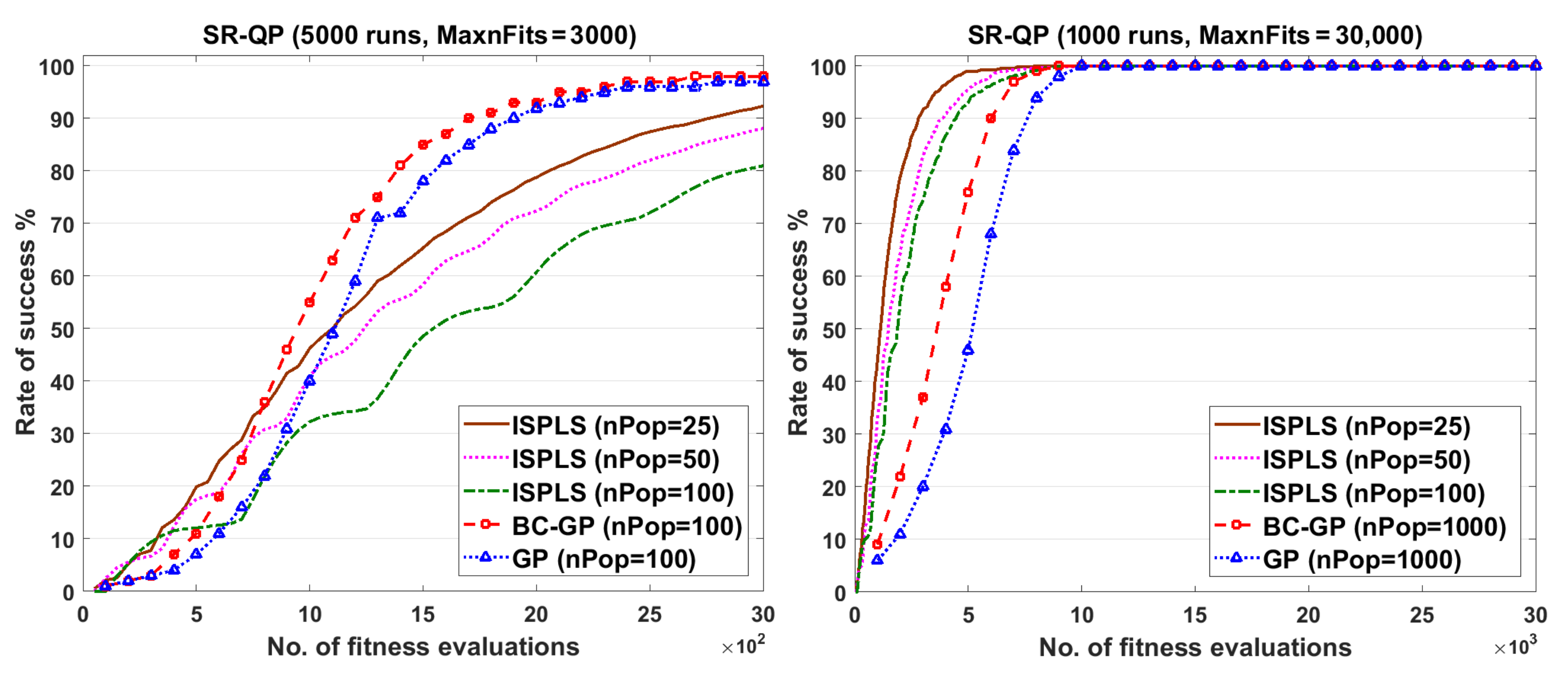
Poli and Langdon [45] used the GP and BC-GP algorithms through two different experiments for the SR-QP problem with different settings. In the first experiment, 5000 independent runs were performed for using for 30 generations, i.e., the maximum number of fitness evaluations for each algorithm was . In the second experiment, 1000 independent runs were performed using for 30 generations, i.e., the maximum number of fitness evaluations for each algorithm was = 30,000. Similar experiments were conducted for the POLY-4 problem, where 5000 independent runs and other 1000 independent runs were performed with and = 10,000, respectively. For each run, the GP and BC-GP algorithms iterated for 30 generations, i.e., = 30,000 and = 300,000 fitness evaluations. Results of the GP and BC-GP algorithms are obtained from [46].
For the ISPLS algorithm, six different experiments were conducted for the SR-SP problem using different settings. Mainly, 5000 independent runs with , and 1000 independent runs with = 30,000 were performed, where each experiment was repeated three times using and . The remaining parameter values of the ISPLS algorithm are shown in Table 1. Figure 4 shows the performance of the proposed algorithm compared with the GP and BC-GP algorithms in terms of the rate of success for the SR-QP problem.
For the POLY-4 problem, we repeated the same experiments of the SR-QP problem using the ISPLS algorithms. Specifically, 5000 independent runs with = 30,000, and 1000 independent runs with = 300,000 were performed and repeated three times using and . The remaining parameter values of the ISPLS algorithm are shown in Table 1. Figure 5 shows the performance of all algorithms in terms of the rate of success for the POLY-4 problem.
As noticed from the previous figures, the ISPLS algorithm can find an optimal solution very fast compared with the BC-GP and GP algorithms. Therefore, the ISPLS algorithm can save a lot of time and computations during the search process. One can conclude that ISPLS was superior to GP and BC-GP.
5.3.3. ISPLS Algorithm vs. CGP, ECGP, EGGP, TAPMCGP and FMCGP Algorithms
Walker and Miller in [39], Atkinson in [47] and Fang and Joe in [48] examined the performance of different versions of the Cartesian genetic programming (CGP) algorithm. Specifically, extensive numerical experiments have been performed on many benchmark problems using the CGP, ECGP, EGGP, TAPMCGP, and FMCGP algorithms. In this experiment, we present a comparison between the performance of these algorithms and the performance of the ISPLS algorithm. For the CGP and ECGP algorithms in [39], 50 independent runs were performed for each problem under study. However, for the CGP, EGGP, TAPMCGP, and FMCGP algorithms in [47,48], 100 independent runs were performed for each problem under study. Similarly, we also performed 100 independent runs for each problem using the ISPLS algorithm. For each run, the algorithm ran until an optimal solution with the maximum fitness value was discovered. The parameter values of the ISPLS algorithm for each problem are shown in Table 1. Moreover, we used , and for the SR-QUP, SR-SP and 3-BEP problems, respectively.
Table 5 shows the performance of the CGP, ECGP, EGGP and ISPLS algorithms in terms of the median (ME), median standard deviation (MAD) and interquartile range (IQR) of the number of fitness evaluations used to reach the optimal solution, where results of CGP, ECGP and EGGP were reported from the original references [39,47]. Table 6 shows the performance of Baseline CGP, TAPMCGP, FMCGP and ISPLS algorithms in terms of the mean and standard deviation (Std) of the number of fitness evaluations used to reach the optimal solution, where results of Baseline CGP, TAPMCGP, and FMCGP were reported from its original reference [48]. A one-sample t-test, two-tailed, was used to compare the significant differences between the means of the Baseline CGP, TAPMCGP, and FMCGP versus ISPLS, where means the difference is very significant, means the difference is very significant, and means the difference is not significant.
From results in Table 5 and Table 6, we can see that the ISPLS algorithm clearly outperforms all algorithms under consideration for all test problems, except the FMCGP algorithm for the SR-SP problem. These results reflect the power of the LS procedure with the the proposed breeding operator: shaking, grafting and pruning operators.
6. Conclusions
The ISPLS algorithm is proposed as an extension of the AIS algorithm, which is a popular population-based meta-heuristic method. Solution representation can be distinguished as the main difference between ISPLS and AIS algorithms. More specifically, solutions in the ISPLS algorithm are computer programs represented by parse trees. In addition, the proposed sets of local search procedures are used to define and explore the best neighborhoods of a solution. This procedure is able to balance between the intensification and the diversification searches. Three types of standard problems were used to test the performance of the ISPLS algorithm through a set of experiments to analyze the main parameters of the proposed algorithm. From these numerical experiments, the ISPLS algorithm showed promising performance compared to different versions of the GP algorithm. Specifically, the ISPLS algorithm outperformed the GP algorithm in terms of success rate and also the required number of fitness evaluations to reach an optimal solution, at least for the well-studied test problems.
Author Contributions
Conceptualization, E.M., Y.R. and A.-R.H.; methodology, E.M., Y.R. and A.-R.H.; programming and implementation, E.M., Y.R. and A.-R.H.; writing—original draft preparation, E.M. and Y.R.; writing—review and editing, E.M., Y.R. and A.-R.H. All authors have read and agreed to the published version of the manuscript.
Funding
This research received no external funding.
Data Availability Statement
Main results of the paper attached as Excel file.
Conflicts of Interest
The authors declare no conflict of interest.
References
- Gendreau, M.; Potvin, J.Y. Handbook of Metaheuristics; Springer: Berlin/Heidelberg, Germany, 2010; Volume 2. [Google Scholar]
- Koza, J.R. Genetic Programming: A Paradigm for Genetically Breeding Populations of Computer Programs to Solve Problems; Stanford University: Stanford, CA, USA, 1990. [Google Scholar]
- Koza, J.R. Genetic Programming: On the Programming of Computers by Means of Natural Selection; MIT Press: Cambridge, MA, USA, 1992; Volume 1. [Google Scholar]
- Cramer, N.L. A representation for the adaptive generation of simple sequential programs. In Proceedings of the First International Conference on Genetic Algorithms, Pittsburgh, PA, USA, 24–26 July 1985; pp. 183–187. [Google Scholar]
- Koza, J.R. Genetic programming as a means for programming computers by natural selection. Stat. Comput. 1994, 4, 87–112. [Google Scholar] [CrossRef]
- Koza, J.R. Genetic Programming III: Darwinian Invention and Problem Solving; Morgan Kaufmann: Burlington, MA, USA, 1999; Volume 3. [Google Scholar]
- Santoso, L.; Singh, B.; Rajest, S.; Regin, R.; Kadhim, K. A genetic programming approach to binary classification problem. EAI Endorsed Trans. Energy Web 2020, 8, e11. [Google Scholar] [CrossRef]
- Devarriya, D.; Gulati, C.; Mansharamani, V.; Sakalle, A.; Bhardwaj, A. Unbalanced breast cancer data classification using novel fitness functions in genetic programming. Expert Syst. Appl. 2020, 140, 112866. [Google Scholar] [CrossRef]
- Hu, N.; Zhong, J.; Zhou, J.T.; Zhou, S.; Cai, W.; Monterola, C. Guide them through: An automatic crowd control framework using multi-objective genetic programming. Appl. Soft Comput. 2018, 66, 90–103. [Google Scholar] [CrossRef] [Green Version]
- De Vega, F.F.; Olague, G.; Lanza, D.; Banzhaf, W.; Goodman, E.; Menendez-Clavijo, J.; Martinez, A. Time and individual duration in genetic programming. IEEE Access 2020, 8, 38692–38713. [Google Scholar] [CrossRef]
- De Giorgi, M.G.; Quarta, M. Hybrid multigene genetic programming-artificial neural networks approach for dynamic performance prediction of an aeroengine. Aerosp. Sci. Technol. 2020, 103, 105902. [Google Scholar] [CrossRef]
- Zhang, F.; Mei, Y.; Nguyen, S.; Zhang, M. Collaborative multifidelity-based surrogate models for genetic programming in dynamic flexible job shop scheduling. IEEE Trans. Cybern. 2021. [Google Scholar] [CrossRef]
- Hodan, D.; Mrazek, V.; Vasicek, Z. Semantically-oriented mutation operator in cartesian genetic programming for evolutionary circuit design. Genet. Program. Evolvable Mach. 2021, 22, 539–572. [Google Scholar] [CrossRef]
- Dray, K.E.; Edelstein, H.I.; Dreyer, K.S.; Leonard, J.N. Control of mammalian cell-based devices with genetic programming. Curr. Opin. Syst. Biol. 2021, 28, 100372. [Google Scholar] [CrossRef]
- Alviso, D.; Artana, G.; Duriez, T. Prediction of biodiesel physico-chemical properties from its fatty acid composition using genetic programming. Fuel 2020, 264, 116844. [Google Scholar] [CrossRef]
- Huang, J.; Liew, J.; Ademiloye, A.; Liew, K.M. Artificial intelligence in materials modeling and design. Arch. Comput. Methods Eng. 2021, 28, 3399–3413. [Google Scholar] [CrossRef]
- Zhong, J.; Feng, L.; Cai, W.; Ong, Y.S. Multifactorial genetic programming for symbolic regression problems. IEEE Trans. Syst. Man Cybern. Syst. 2018, 50, 4492–4505. [Google Scholar] [CrossRef]
- Chaabene, W.B.; Nehdi, M.L. Genetic programming based symbolic regression for shear capacity prediction of SFRC beams. Constr. Build. Mater. 2021, 280, 122523. [Google Scholar] [CrossRef]
- Gayanov, R.; Mironov, K.; Kurennov, D. Estimating the trajectory of a thrown object from video signal with use of genetic programming. In Proceedings of the 2017 IEEE International Symposium on Signal Processing and Information Technology (ISSPIT), Bilbao, Spain, 18–20 December 2017; pp. 134–138. [Google Scholar]
- Pigozzi, F.; Medvet, E.; Nenzi, L. Mining Road Traffic Rules with Signal Temporal Logic and Grammar-Based Genetic Programming. Appl. Sci. 2021, 11, 10573. [Google Scholar] [CrossRef]
- Mabrouk, E.; Ayman, A.; Raslan, Y.; Hedar, A.R. Immune system programming for medical image segmentation. J. Comput. Sci. 2019, 31, 111–125. [Google Scholar] [CrossRef]
- Meier, A.; Gonter, M.; Kruse, R. Accelerating convergence in cartesian genetic programming by using a new genetic operator. In Proceedings of the 15th Annual Conference on Genetic and Evolutionary Computation, Amsterdam, The Netherlands, 6–10 July 2013; pp. 981–988. [Google Scholar]
- Montoya, F.G.; Navarro, R.B. Optimization Methods Applied to Power Systems: Volume 1; MDPI: Basel, Switzerland, 2019. [Google Scholar]
- Adam, S.P.; Alexandropoulos, S.A.N.; Pardalos, P.M.; Vrahatis, M.N. No free lunch theorem: A review. In Approximation and Optimization; Springer: Cham, Switzerland, 2019; pp. 57–82. [Google Scholar]
- Mabrouk, E.; Hedar, A.R.; Fukushima, M. Memetic programming with adaptive local search using tree data structures. In Proceedings of the 5th International Conference on Soft Computing as Transdisciplinary Science and Technology, Cergy-Pontoise, France, 28–31 October 2008; pp. 258–264. [Google Scholar]
- Hedar, A.R.; Mabrouk, E.; Fukushima, M. Tabu programming: A new problem solver through adaptive memory programming over tree data structures. Int. J. Inf. Technol. Decis. Mak. 2011, 10, 373–406. [Google Scholar] [CrossRef]
- Osman, M.K. Designing Machine Learning Tools Based on Meta-Heuristic Programming. Ph.D. Thesis, University of Cairo, Cairo, Egypt, 2011. [Google Scholar]
- Saleh, A.J.; Karim, A.; Shanmugam, B.; Azam, S.; Kannoorpatti, K.; Jonkman, M.; Boer, F.D. An intelligent spam detection model based on artificial immune system. Information 2019, 10, 209. [Google Scholar] [CrossRef] [Green Version]
- Park, H.; Choi, J.E.; Kim, D.; Hong, S.J. Artificial immune system for fault detection and classification of semiconductor equipment. Electronics 2021, 10, 944. [Google Scholar] [CrossRef]
- Mabrouk, E. Meta-Heuristics Programming and Its Applications. Ph.D. Thesis, University of Kyoto, Kyoto, Japan, 2011. [Google Scholar]
- Talbi, E. Metaheuristics: From Design to Implementation; John Wiley & Sons: Hoboken, NJ, USA, 2009. [Google Scholar]
- De Castro, L.N.; Timmis, J. Artificial immune systems as a novel soft computing paradigm. Soft Comput. 2003, 7, 526–544. [Google Scholar] [CrossRef]
- Bondal, A.A. Artificial Immune Systems Applied to Job Shop Scheduling. Ph.D. Thesis, Ohio University, Athens, OH, USA, 2008. [Google Scholar]
- Gonzalez, F.; Dasgupta, D. A Study of Artificial Immune Systems Applied to Anomaly Detection. Ph.D. Thesis, University of Memphis, Memphis, TN, USA, 2003. [Google Scholar]
- Farmer, J.D.; Packard, N.H.; Perelson, A.S. The immune system, adaptation, and machine learning. Phys. D Nonlinear Phenom. 1986, 22, 187–204. [Google Scholar] [CrossRef]
- Aickelin, U.; Greensmith, J.; Twycross, J. Immune system approaches to intrusion detection—A review. In Artificial Immune Systems; Springer: Berlin/Heidelberg, Germany, 2004; pp. 316–329. [Google Scholar]
- Brownlee, J. Clonal Selection Theory & CLONALG—The Clonal Selection Classification Algorithm (CSCA); Technical Report; Swinburne University of Technology: Melbourne, VIC, Australia, 2005. [Google Scholar]
- Al-Enezi, J.; Abbod, M.; Alsharhan, S. Artificial immune systems-models, algorithms and applications. IJRRAS 2010, 3, 118–131. [Google Scholar]
- Walker, J.A.; Miller, J.F. The automatic acquisition, evolution and reuse of modules in cartesian genetic programming. Evol. Comput. IEEE Trans. 2008, 12, 397–417. [Google Scholar] [CrossRef]
- Gangopadhyay, D.; Reyhani-Masoleh, A. Multiple-bit parity-based concurrent fault detection architecture for parallel CRC computation. IEEE Trans. Comput. 2015, 65, 2143–2157. [Google Scholar] [CrossRef]
- Walker, J.A.; Miller, J.F. Evolution and acquisition of modules in cartesian genetic programming. In Genetic Programming; Springer: Berlin/Heidelberg, Germany, 2004; pp. 187–197. [Google Scholar]
- Steel, R.G.D.; Torrie, J.H.; Dicky, D.A. Principles and Procedures of Statistics: A Biometrical Approach; McGraw-Hill: New York, NY, USA, 1997. [Google Scholar]
- Silva, S.; Almeida, J. GPLAB–A Genetic Programming Toolbox for MATLAB. 2003. Available online: http://gplab.sourceforge.net/ (accessed on 10 March 2022).
- William, E.; Northern, J., III. Genetic programming lab (GPLab) tool set version 3.0. In Proceedings of the Region 5 Conference, 2008 IEEE, Kansas City, MO, USA, 17–20 April 2008; pp. 1–6. [Google Scholar]
- Poli, R. Tournament selection, iterated coupon-collection problem, and backward-chaining evolutionary algorithms. In Foundations of Genetic Algorithms; Springer: Berlin/Heidelberg, Germany, 2005; pp. 132–155. [Google Scholar]
- Poli, R.; Langdon, W.B. Backward-chaining evolutionary algorithms. Artif. Intell. 2006, 170, 953–982. [Google Scholar] [CrossRef] [Green Version]
- Atkinson, T. Evolving Graphs by Graph Programming. Ph.D. Thesis, University of York, York, UK, 2019. [Google Scholar]
- Fang, W.; Gu, M. FMCGP: Frameshift mutation cartesian genetic programming. Complex Intell. Syst. 2021, 7, 1195–1206. [Google Scholar] [CrossRef]
Figure 1.
Flowchart of the CLONALG algorithm [32].
Figure 1.
Flowchart of the CLONALG algorithm [32].

Figure 2.
Generating new programs using shaking, grafting and pruning procedures [30].
Figure 2.
Generating new programs using shaking, grafting and pruning procedures [30].

Figure 3.
Flowchart of the LS procedure.

Figure 4.
Performance of ISPLS, BC-GP, and GP algorithms for the SR-QP problem.

Figure 5.
Performance of ISPLS, BC-GP and GP algorithms for the POLY-4 problem.


Table 1.
Standard values of ISPLS parameters for the test problems.
| Parameter | |||||||
|---|---|---|---|---|---|---|---|
| SR-QP | 3 | 25 | 0.2 | 1 | 0.5 | 0.25 | 0.04 |
| SR-QUP | 4 | 50 | 0.2 | 1 | 0.6 | 0.25 | 0.04 |
| SR-SP | 4 | 75 | 0.2 | 1 | 0.5 | 0.25 | 0.06 |
| POLY-4 | 3 | 50 | 0.2 | 2 | 0.5 | 0.25 | 0.06 |
| 6-BM | 4 | 50 | 0.2 | 2 | 0.5 | 0.25 | 0.04 |
| 3-BEP | 5 | 50 | 0.2 | 2 | 0.5 | 0.25 | 0.04 |
Table 2.
ISPLS performance under different values of parameters and .
| Parameter | SR-QP | SR-QUP | SR-SP | POLY-4 | 6-BM | 3-BEP | |
|---|---|---|---|---|---|---|---|
| Name | Value | Mean | Mean | Mean | Mean | Mean | Mean |
| 2 | 2252 | 46,013 | 16,699 | 4560 | 15,880 | 70,359 | |
| 3 | 1166 | 15,794 | 13,242 | 5326 | 9689 | 74,225 | |
| 4 | 1360 | 8485 | 7867 | 6855 | 9300 | 10,480 | |
| 5 | 2920 | 6334 | 7415 | 24,225 | 8928 | 3036 | |
| 6 | 9060 | 15,662 | 19,366 | - | 9404 | 2539 | |
| 25 | 1170 | 9141 | 14,731 | 4708 | 9604 | 2822 | |
| 50 | 1422 | 8927 | 10,606 | 4694 | 7679 | 3512 | |
| 75 | 1641 | 9122 | 10,177 | 5599 | 9660 | 3400 | |
| 100 | 2118 | 8652 | 11,475 | 5941 | 11,644 | 3035 | |
| 125 | 1764 | 8536 | 13,330 | 6729 | 9534 | 3254 | |
| 0.05 | 1835 | 8361 | 12,815 | 9184 | 21,363 | 3948 | |
| 0.1 | 1541 | 8839 | 10,346 | 7066 | 11,886 | 3032 | |
| 0.15 | 1099 | 7498 | 10,322 | 5796 | 10,730 | 2911 | |
| 0.2 | 1213 | 8503 | 9147 | 4956 | 10,747 | 2841 | |
| 0.25 | 1202 | 8311 | 7824 | 5276 | 8875 | 3290 | |
Table 3.
ISPLS performance under different values of parameters and .
| Parameter | SR-QP | SR-QUP | SR-SP | POLY-4 | 6-BM | 3-BEP | |
|---|---|---|---|---|---|---|---|
| Name | Value | Mean | Mean | Mean | Mean | Mean | Mean |
| 1 | 1447 | 8431 | 8310 | 4441 | 9747 | 3459 | |
| 2 | 1362 | 8671 | 9099 | 4959 | 9298 | 2921 | |
| 3 | 1354 | 7874 | 9030 | 6042 | 8188 | 2656 | |
| 4 | 1644 | 8715 | 8032 | 6504 | 9050 | 3023 | |
| 5 | 1425 | 12,526 | 9817 | 6976 | 9770 | 2884 | |
| 0.3 | 1213 | 13,169 | 8706 | 4512 | 8370 | 2363 | |
| 0.4 | 1132 | 10,357 | 7299 | 5030 | 7977 | 2344 | |
| 0.5 | 1216 | 8688 | 9047 | 5406 | 8940 | 3022 | |
| 0.6 | 1242 | 7717 | 10,398 | 5628 | 10,673 | 3024 | |
| 0.7 | 1385 | 8422 | 9518 | 5598 | 10,905 | 2848 | |
| 0.2 | 1311 | 11,170 | 9871 | 5083 | 9464 | 2842 | |
| 0.25 | 1348 | 8097 | 9267 | 5190 | 8755 | 3285 | |
| 0.3 | 1207 | 9813 | 9936 | 4943 | 8689 | 2778 | |
| 0.35 | 1345 | 7413 | 8887 | 5287 | 9638 | 2979 | |
| 0.4 | 1343 | 8863 | 7221 | 4694 | 8426 | 2847 | |
| 0.02 | 1180 | 8105 | 10,449 | 4407 | 9984 | 3591 | |
| 0.03 | 1387 | 10,238 | 7885 | 4081 | 9668 | 3369 | |
| 0.04 | 1310 | 8879 | 7675 | 4176 | 9585 | 3220 | |
| 0.05 | 1238 | 8593 | 8596 | 5293 | 8177 | 2660 | |
| 0.06 | 1203 | 11,130 | 9115 | 4680 | 8401 | 3038 | |
Table 4.
Comparison of GPLab, TP and ISPLS algorithms under the same limitations on the number of fitness evaluations, where means “not significantly different”, means “significantly different”, and means “highly significant”.
Table 4.
Comparison of GPLab, TP and ISPLS algorithms under the same limitations on the number of fitness evaluations, where means “not significantly different”, means “significantly different”, and means “highly significant”.
| GPLab | TP | ISPLS | ||||||
|---|---|---|---|---|---|---|---|---|
| Problem | Mean | Rate | Value | Mean | Rate | Value | Mean | Rate |
| SR-QP | 1303 | 81% | 0.011 | 801 | 99% | <0.01 | 1129 | 97% |
| 6-BM | 8445 | 100% | 0.0879 | 7829 | 98% | 0.6410 | 7599 | 98% |
| 3-BEP | 11,175 | 77% | <0.01 | 5612 | 100% | <0.01 | 2363 | 100% |
Table 5.
Comparison of CGP, ECGP, EGGP and ISPLS algorithms, in terms of ME, MAD, and IQR. All values are expressed in terms of thousands.
Table 5.
Comparison of CGP, ECGP, EGGP and ISPLS algorithms, in terms of ME, MAD, and IQR. All values are expressed in terms of thousands.
| Problem | CGP | ECGP | CGP | EGGP | ISPLS | |
|---|---|---|---|---|---|---|
| [39] | [39] | [47] | [47] | |||
| ME | 32.2 | 25.9 | – | – | 3.5 | |
| SR-QUP | MAD | 31.0 | 24.4 | – | – | 6.9 |
| IQR | 525.6 | 296.8 | – | – | 5.9 | |
| ME | 12.7 | 29.7 | – | – | 4.6 | |
| SR-SP | MAD | 10.9 | 25.1 | – | – | 5.4 |
| IQR | 64.1 | 279.4 | – | – | 6.2 | |
| ME | 6.0 | 5.9 | 4.4 | 2.8 | 1.5 | |
| 3-BEP | MAD | 2.9 | 3.8 | 2.5 | 1.6 | 1.6 |
| IQR | 6.6 | 10.4 | 5.3 | 4.8 | 2.4 |
Table 6.
Comparison of CGP, TAPMCGP, FMCGP and ISPLS algorithms, in terms of mean and Std, where means “not significantly different”, means “significantly different”, and means “highly significant”.
Table 6.
Comparison of CGP, TAPMCGP, FMCGP and ISPLS algorithms, in terms of mean and Std, where means “not significantly different”, means “significantly different”, and means “highly significant”.
| Problem | Baseline CGP | TAPMCGP | FMCGP | ISPLS | |
|---|---|---|---|---|---|
| [48] | [48] | [48] | |||
| Mean | 28,633.66 | 7150.55 | 10,537.45 | 6333.97 | |
| SR-QUP | Std | 51,655.34 | 15,221.36 | 16,538.50 | 6276.15 |
| p value | <0.01 | 0.1962 | <0.01 | ||
| Mean | 15,843.74 | 6832.54 | 5676.55 | 7221.01 | |
| SR-SP | Std | 25,609.54 | 12,326.49 | 5865.20 | 7591.74 |
| p value | <0.01 | 0.6100 | 0.044 |
Publisher’s Note: MDPI stays neutral with regard to jurisdictional claims in published maps and institutional affiliations. |
© 2022 by the authors. Licensee MDPI, Basel, Switzerland. This article is an open access article distributed under the terms and conditions of the Creative Commons Attribution (CC BY) license (https://creativecommons.org/licenses/by/4.0/).
Share and Cite
MDPI and ACS Style
Mabrouk, E.; Raslan, Y.; Hedar, A.-R. Immune System Programming: A Machine Learning Approach Based on Artificial Immune Systems Enhanced by Local Search. Electronics 2022, 11, 982. https://doi.org/10.3390/electronics11070982
AMA Style
Mabrouk E, Raslan Y, Hedar A-R. Immune System Programming: A Machine Learning Approach Based on Artificial Immune Systems Enhanced by Local Search. Electronics. 2022; 11(7):982. https://doi.org/10.3390/electronics11070982
Chicago/Turabian StyleMabrouk, Emad, Yara Raslan, and Abdel-Rahman Hedar. 2022. "Immune System Programming: A Machine Learning Approach Based on Artificial Immune Systems Enhanced by Local Search" Electronics 11, no. 7: 982. https://doi.org/10.3390/electronics11070982
Note that from the first issue of 2016, this journal uses article numbers instead of page numbers. See further details here.