
Automatic Calibration of Piezoelectric Bed-Leaving Sensor Signals Using Genetic Network Programming Algorithms


1
Faculty of Software and Information Science, Iwate Prefectural University, Takizawa City 020-0693, Japan
2
Faculty of Systems Science and Technology, Akita Prefectural University, Yurihonjo City 015-0055, Japan
*
Author to whom correspondence should be addressed.
†
These authors contributed equally to this work.
Algorithms 2021, 14(4), 117; https://doi.org/10.3390/a14040117
Submission received: 8 March 2021
/
Revised: 27 March 2021
/
Accepted: 2 April 2021
/
Published: 4 April 2021
(This article belongs to the Section Evolutionary Algorithms and Machine Learning)
Abstract
:This paper presents a filter generating method that modifies sensor signals using genetic network programming (GNP) for automatic calibration to absorb individual differences. For our earlier study, we developed a prototype that incorporates bed-leaving detection sensors using piezoelectric films and a machine-learning-based behavior recognition method using counter-propagation networks (CPNs). Our method learns topology and relations between input features and teaching signals. Nevertheless, CPNs have been insufficient to address individual differences in parameters such as weight and height used for bed-learning behavior recognition. For this study, we actualize automatic calibration of sensor signals for invariance relative to these body parameters. This paper presents two experimentally obtained results from our earlier study. They were obtained using low-accuracy sensor signals. For the preliminary experiment, we optimized the original sensor signals to approximate high-accuracy ideal sensor signals using generated filters. We used fitness to assess differences between the original signal patterns and ideal signal patterns. For application experiments, we used fitness calculated from the recognition accuracy obtained using CPNs. The experimentally obtained results reveal that our method improved the mean accuracies for three datasets.
1. Introduction
The progression of longevity is forcing humanity to confront various unprecedented social problems. In hyper-aged societies, both healthy and unhealthy life expectancy lifespans are increasing year by year [1]. Elderly people with longevity invariably spend longer periods of their second life outside their homes because they are living longer without severe disability [2]. Hospitals and nursing-care facilities are now confronting daunting labor shortages in terms of medical doctors, nurses and caretakers. Especially during nighttime, labor shortages can lead to accidents of various types, particularly related to numerous fall and tumble risks. According to a report by Mita et al. [3], fall accidents occurred as approximately half the total number of accidents that occur among elderly people at nursing-care facilities. Most fall accidents occurred when patients left their own bed.
Providing suitable solutions with assessment primarily requires fall accident prevention. Recently, bed-leaving sensors have come to be used widely at hospitals and nursing-care facilities to prevent fall-related behaviors in advance. A method of detecting abnormal behavior patterns has been proposed for monitoring sleeping elderly people [4]. One can imagine that in a psychiatric ward, however, it would be unrealistic to use a camera without some special justification. Especially for hospitals and nursing-care facilities, the use of cameras for monitoring patients is limited for reasons of privacy and morality, except for intensive care units or special wards for infectious diseases. To assess privacy considerations, a fall detection method using radio-frequency identification devices (RFIDs) has been proposed to detect changes of electrical intensity [5]. Nevertheless, detection using that method is limited to a person’s status after a fall. For the development of bed-leaving sensors, various factors exist for consideration in terms of system reliability, stability, durability, initial and maintenance cost, detection speed, privacy, and quality of life (QoL) for patients.
We proposed a bed-leaving sensor system [6] using piezoelectric films bound with acrylic resin boards to detect pressure. An important benefit of this approach is that it can be installed in off-the-shelf beds. Sensors installed between a bed and a cover can detect a person’s behaviors. We evaluated basic sensor characteristics and the relation between accuracy and body parameters such as the weight and height of subjects [6]. Moreover, we evaluated our originally developed sensor system using discontinuous datasets that comprised random behavior patterns [6]. However, counter-propagation networks (CPNs) [7] used for bed-leaving behavior recognition are insufficient to incorporate individual differences in physique such as weight and height. Especially for low-weight subjects, recognition accuracies were dramatically lower. To address this difficulty, we propose a method for automatically generating a filter set for shaping sensor signals based on evolutionary learning (EL) to demonstrate automatic sensor calibration according to subjects.
The remainder of the paper is structured as follows—in Section 2, related studies of EL-based calibration methods are reviewed for improving classification and recognition accuracy. Section 3 and Section 4 respectively present our proposed method and our original sensor signal datasets. Subsequently, Section 5 and Section 6 present a preliminary experiment result obtained using a dataset obtained from a particular sensor, in addition to application experiment results obtained using three datasets obtained from one person for whom low initial recognition accuracy was obtained compared to those of other experiment participants. Section 7 presents our analyses of the properties of parameters and node changes for additional optimization. Finally, Section 8 concludes our presentation of the present work and highlights future work. As described herein, we use our proposed fundamental method with originally developed sensors of two types [8]. To explain our present study, we have included additional details in Section 2, Section 6 and Section 7.
2. Related Studies
As a framework for resolving difficulties combined with learning, inferring, and optimizing, EL-based methods are used widely in numerous applications [9]. Song et al. [10] proposed a method to generate filters used for electrocardiogram signals based on a genetic algorithm (GA) [11]. The limitation of GAs is that they are merely applicable to parameter optimization. Koza [12] proposed genetic programming (GP) for use as a unified method to evolve programs affected by living things. To apply program generation, learning, reasoning, and conceptual formation, GP can be extended to accommodate a structural representation of GA genotypes. Moreover, GP can express data structures and programs as trees and graphs. For an extension to graph structures, genetic network programming (GNP) was proposed for efficient searching while avoiding tree bloat.
As pioneer work, Katagiri et al. [13,14] and Hirasawa et al. [15] have proposed original frameworks of GNP that obtained intelligent behavior sequences for evolutionary robotics. Furthermore, they automatically designed complex systems based on evolutionary optimization techniques such as GA and GP. They [16] evaluated GNP using the partially observable Markov decision process (POMDP) problem developed by Goldman et al. [17]. The experimentally obtained simulation results elucidated that GNP evolved more effectively than GP. Especially, premature convergence occurs only rarely in GNP compared to its more common occurrence in GP. Moreover, the fitness of GNP has been reported as higher than that of GP from the initial generation.
Mabu et al. [18] combined GNP with reinforcement learning [19] to create dynamic graph structures. They also used the POMDP problem [17] for benchmarking. The experimentally obtained results demonstrated that their method presents advantages over conventional methods based on GP and EP. Moreover, Chen et al. [20] combined GNP with Sarsa learning [21] for stock market trading to judge the timing of buying and selling. The experimentally obtained simulation results obtained using stock price datasets of 16 brands during four years clarified that the fitness and profits of their composed method were higher than the existing stock prediction methods.
Li et al. [22] combined GNP with distributed estimation algorithms to solve traffic prediction problems based on class association rule mining. They used a probabilistic model that enhanced ultimate objective evolution. The experimentally obtained simulation results revealed that their method extracted class rules more effectively, especially for a case of an increased number of class association candidate rules. Moreover, the classification accuracy of their method achieved sufficient results for traffic prediction systems. Li et al. [23] also combined GNP with a hybrid probabilistic model-building algorithm to avoid premature convergence and local optima while maintaining population diversity. Their experimentally obtained simulation results, evaluated using a small autonomous robot, demonstrated that their method achieved better performance than any conventional algorithm.
Wedashwara et al. [24] combined GNP with standard dynamic programming to solve knapsack problems [25]. Their method explored suitable combinations of attributes to create clustering and distributed rules. The experimentally obtained simulation results obtained using six benchmark datasets obtained from machine-learning (ML) repositories clarified that their method presents advantages over the use of conventional clustering algorithms such as k-means, hierarchical clustering, fuzzy C means, and affinity propagation. Moreover, their method was found to be suitable for offline processing that specifically emphasizes optimal results rather than short processing time.
Mabu et al. [26] combined GNP with fuzzy set theory [27] for the detection of network intrusions. Experimentally obtained results using two benchmark datasets revealed that their method provided competitively high detection rates when compared with other ML techniques and GNP with the approach of a current cross-industry standard processing for data mining [28]. As the latest study, Mabe et al. [29] combined GNP with a semisupervised learning framework to extract class association rules from a small number of labeled data and from numerous unlabeled data. The experimentally obtained results obtained using several benchmark datasets revealed the classification accuracy of their method as superior to that of conventional methods.
As a graphical model that optimizes parameters and processing structures, GNP is highly independent of classifiers and recognizers. For those reasons, GNP is suitable for combining various existing methods to improve accuracy, especially in practical problems.
3. Proposed Method
3.1. Overall System Structure
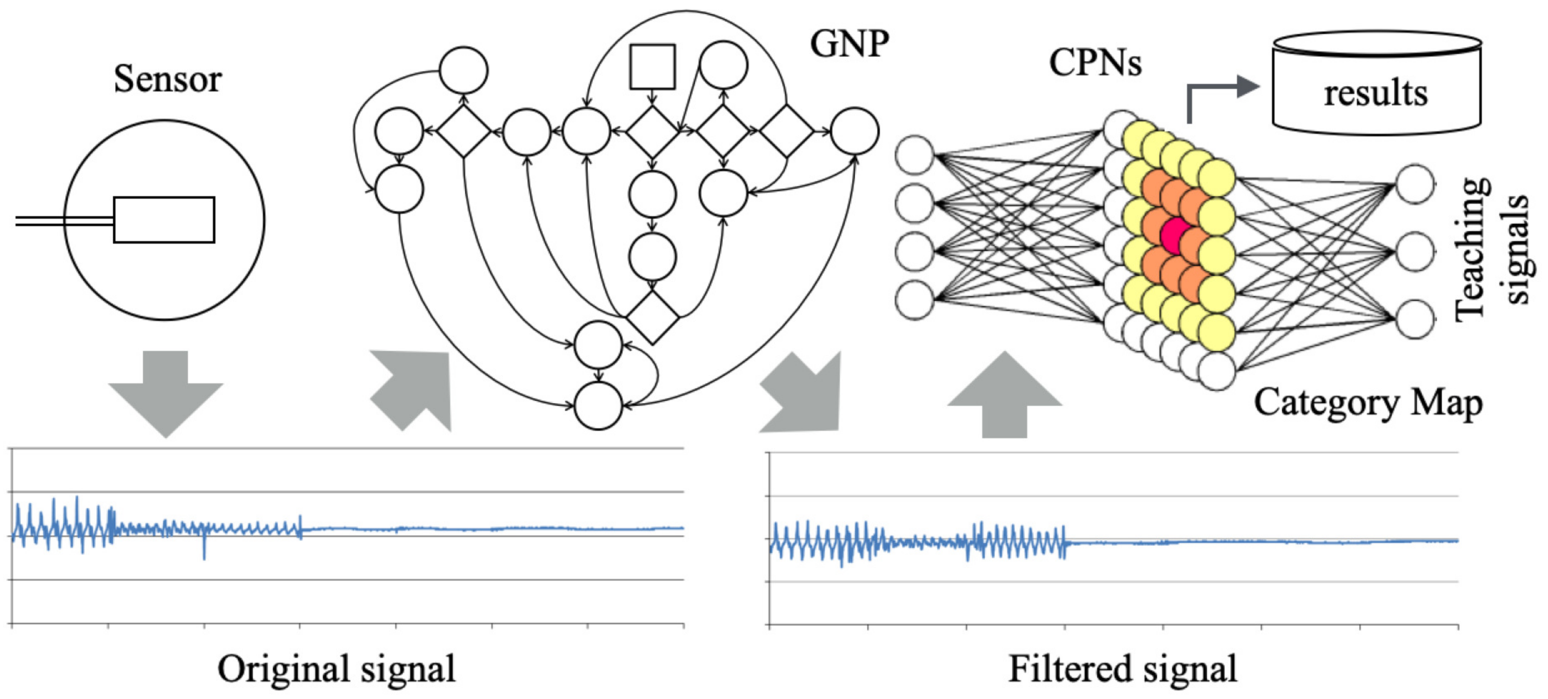
This study was conducted to improve the recognition accuracy of our originally developed bed-leaving detection and behavior pattern recognition system [6]. Our proposed method comprises CPNs combined with GNP that absorbs sensor signal differences as an automatic calibration module. Figure 1 depicts the overall structure of our proposed method, including our originally developed sensor. Sensor signals are obtained from the sensor without an electric power supply because piezoelectric films are used [30]. Subsequently, the obtained sensor signals are modified using GNP. Herein, GNP is optimized in advance using original signals and ideal signals obtained from other datasets that provide superior recognition accuracy. We used CPNs to recognize bed-leaving behavior patterns. The modified sensor signals are presented to CPNs for the training mode of a supervised manner. After training, the network weights on CPNs are fixed. The operation mode of CPNs is then switched from training to validation. Behavior patterns are recognized by CPNs for input sensor signals. For this mode, GNPs are used as a filter. Herein, both GNP and CPNs run rapidly in real time because updating of network structures and weights are terminated for the validation mode.
3.2. Design of GNP Nodes
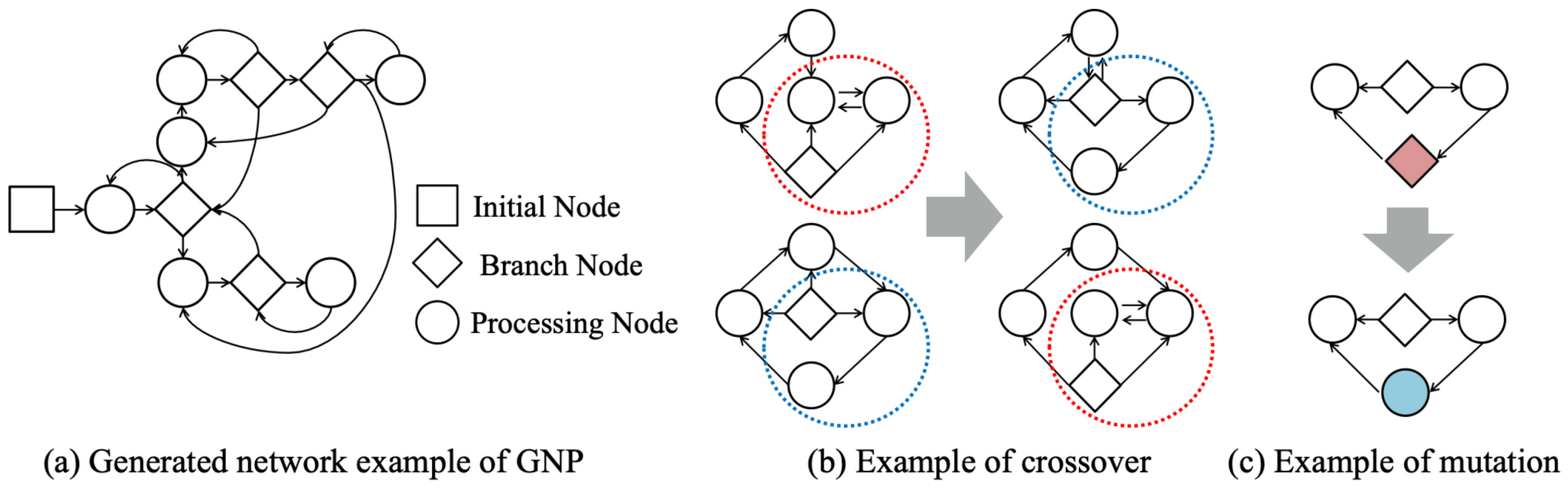
Figure 2a depicts an example of GNP. As an original population, the initial set of nodes is randomly generated. Although GP and GNP use different genotypes such as a tree structure and a graph network structure, the GP tree depth grows infinitely, which is an important benefit for searching when combined with mutation and crossover for an optimal solution. However, an important shortcoming is that it has low searching efficiency if search ranges are expanded. The fitness of nodes near the root is greater than that of nodes near terminals if mutation or crossover occurs near the root. In the early stage of evolution, convergence to a local minimum occurs if a node near the root is unselected. The number of GNP nodes is invariable during the evolution process because it uses a network structure genotype. The influence of fitness for changing nodes is extremely different in the respective nodes.
Figure 2b depicts a crossover example that is applied between two sets of nodes as the following.
- Two sets of nodes are selected randomly.
- Each set of nodes is switched while the connections are maintained.
- New fitness values are calculated.
Figure 2c depicts a mutation example that is applied to a particular node like the following.
- A node is selected randomly.
- A new node is produced randomly.
- The existing node is switched to the new node.
- A new fitness value is calculated.
Throughout the evolutionary process, GNP automatically generates programs as nodes of two types: a branch node and a processing node that respectively comprise a nonterminal symbol and a terminal symbol of GP. We designed 5 branch nodes and 15 processing nodes for filtering original output sensor signals. Table 1 denotes the branch nodes. Each branch node includes three branches compared with two values. Let be an input signal, which is discretized as a 8-bit discrete value versus time t, to a branch node. Herein, d in N5 is defined as
and in N5 is defined as
Table 2 presents processing nodes. Let be an input signal, which is discretized as an 8-bit discrete value versus time t, to a processing node. The processing formulas in each node are the following.
where , , and are gains that adjust the signal strength.
3.3. Counter-Propagation Networks
The rapid progress and development of deep learning (DL) [31] technologies in recent years has contributed remarkably to the classification [32], recognition [33], understanding [34], and prediction [35] of diverse and numerous tasks. With the advent of very deep multilayered backbones such as Inception [36], Xception [37], ResNet [38], ResNeXt [39], and Res2Net [40], the performance and accuracy of DL-based methods significantly outperform those of classical ML-based methods. However, to achieve their full performance, DL-based methods require the combination of large amounts of training and validation data combined with high-dimensional features. Therefore, DL-based methods mainly target large image datasets obtained from various cameras, including depth sensors [41]. For low-dimensional features and low-volume datasets, DL-based methods are unsuitable for training and validation because of the complexity of their networks and their numerous parameters. We infer that conventional DL-based methods have an important role and that they can make a meaningful contribution in this application range.
For this study, we used CPNs [7], which are a conventional ML-based method, to classify and to recognize bed-leaving behavior patterns. Input features from the sensors to the input layer unit i at time t are . A weight from i to Kohonen layer unit j at time t is . Also, a weight from Grossberg layer unit k to Kohonen layer unit j at time t is . Herein, I, J, and K respectively denote the total numbers of input layer units, Kohonen layer units, and Grossberg layer units. Before learning, are initialized randomly. Using the Euclidean distance between and , a winner unit is sought for the following:
A neighborhood region is set from the center of c is
where L stands for the maximum learning iteration. Teaching signals to the Grossberg layer units at time t are . For supervised learning, and in are updated as
where and are learning coefficients that decrease along with learning progress.
4. Bed-Leaving Behavior Datasets
4.1. Sensor and Assignment
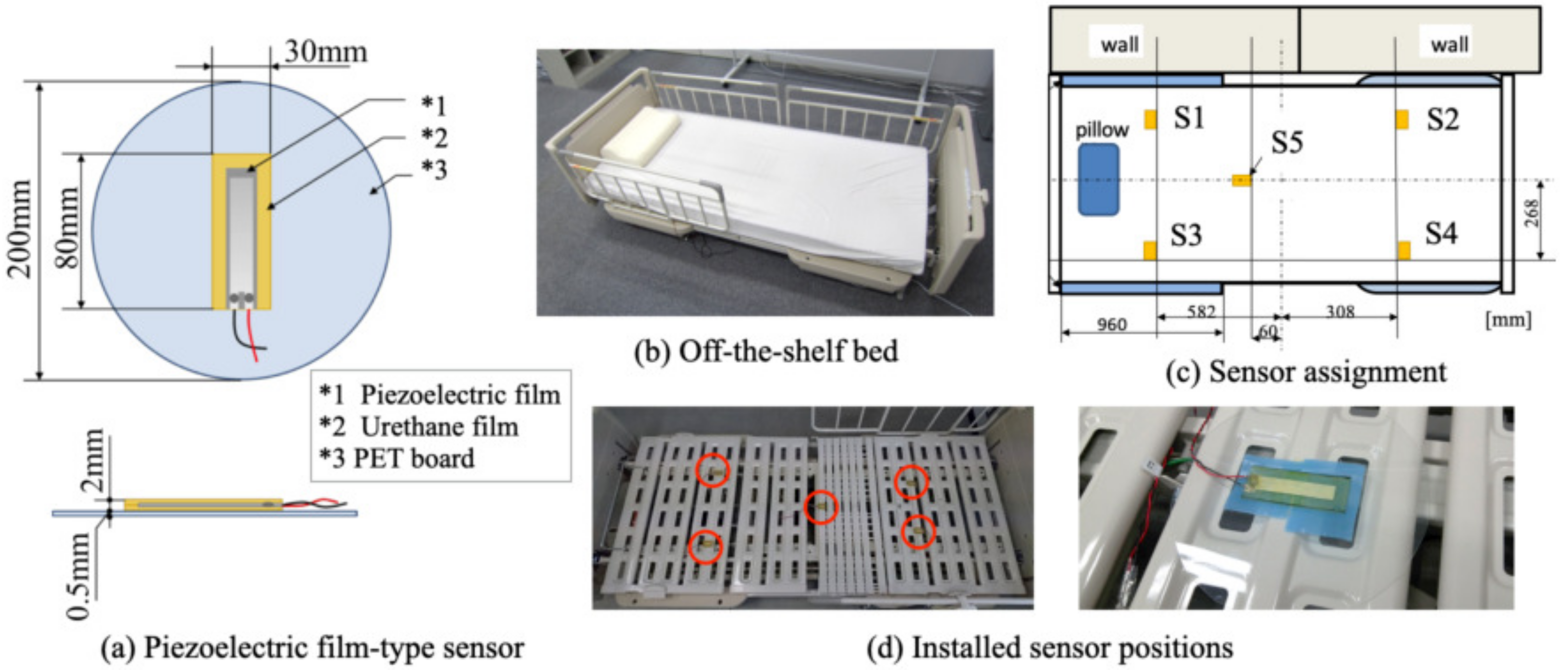
Numerous bed sensors [42] and smart bed systems [43] of various types have been proposed. We proposed the bed-leaving detection system [6] based on ML methods obtained using piezoelectric film-type sensors, as depicted in Figure 3a installed on an off-the-shelf bed. The feature of our sensor system is non-restrictive, invisible, cost-effective, and independent of sensor-driven power. For our latest sensor system, we use only five sensors as the minimum assignment structure, as depicted in Figure 3d. Herein, S1–S5 denote labels of the sensor installation positions. To obtain signals from respective sensors, subjects assumed face-up sleeping, right sleeping, left sleeping, longitudinal sitting, lateral sitting, terminal sitting, and left the bed of seven positions as a single pattern switched at 20 s intervals. We built benchmark datasets used for comparative experiments of bed-leaving detection.
4.2. Target Behavior Patterns
The target behavior patterns for bed-leaving prediction comprise three groups—sleeping, sitting, and leaving [6]. For this study, we attempt to classify detailed behavior patterns from the responses of six sensors. Sleeping can be of three patterns—face-up sleeping, left sleeping, and right sleeping. Sitting can be of three patterns—longitudinal sitting, lateral sitting, and terminal sitting [44]. The total prediction target is to produce seven patterns including leaving. The following are features and estimated sensor responses in each pattern.
- Face-up Sleeping A subject is sleeping on the bed normally to the upper side of the body.Moreover, the person is rolling over on the bed to the right or left side. All the sensors give outputs.
- Longitudinal Sitting A subject is sitting longitudinally on the bed after rising. The sensor response is mainly the output of S5, which is installed on the hip of the subject.
- Lateral Sitting A subject is sitting laterally on the bed after turning the body from longitudinal sitting. The sensor response is that S3 and S4 give outputs. They are installed in the right side of the bed.
- Terminal Sitting A subject is sitting in the terminal position on the bed trying to leave the bed. The sensor response is that none of S1, S2, or S5 gives any output. Moreover, the sensor response is that S3 and S4 give outputs. They are installed near the exit part of the bed. Rapid and correct detection is necessary because of the terminal situation for leaving the bed.
- Left the Bed A subject is leaving the bed. The sensor response is that no sensor gives any output.
Longitudinal sitting is a behavior pattern by which a subject sits up. In numerous cases, a person will return to sleeping. In lateral sitting, a person will move to leave from their bed because they move to turn the body to the terminal. Therefore, our system must determine lateral sitting immediately to predict instances in which a person leaves the bed. Moreover, rapid and correct detection is necessary because of the terminal situation for leaving the bed if a subject moves to longitudinal sitting. We consider that our system can protect patients from injury or accidents caused by falling from the bed because it can detect such phenomena before a subject leaves completely.
4.3. Output Signals and Preprocessing
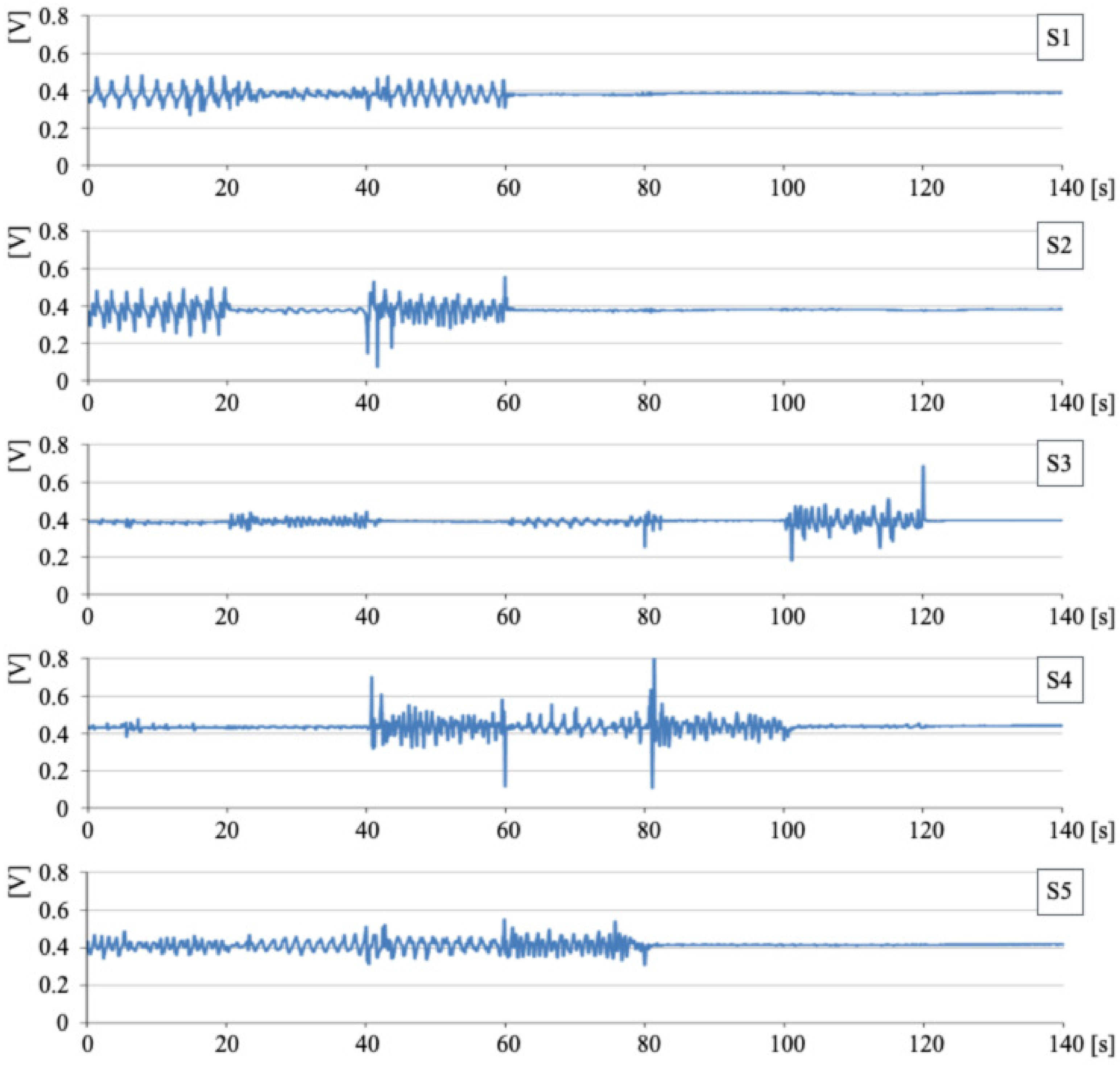
To demonstrate the usefulness of our method, we selected a subject for which the accuracy was 31.9 percentage points lower than those of other subjects in our earlier study [6]. Figure 4 portrays the original sensor signals of the subject. Herein, we set the sampling rate to 50 Hz for recording of the sensor signals. We obtained 7000 signals in each dataset during 140 s. The vertical and horizontal axes in the figures respectively depict the sensor output voltage and signals. From the 6000th to 7000th signals, we can infer that the subject left the bed completely. Sensor signals show no output in this range because there is no load to the sensors. Therefore, we removed this range from the processing target as filtering.
5. Preliminary Experiment
5.1. Setup and Evaluation Criteria
We applied GNP to low-accuracy sensor signals for the correction of high-accuracy sensor signals as ideal sensor signals. This optimization is based on evolutionary image processing [45]. The optimization goal of this image processing was set to ideal images that were selected from ground-truth image datasets. Although ideal sensor signals differ among subjects, we inferred that accuracy had improved if low-accuracy sensor signals were approximated to high-accuracy sensor signals. We set high-accuracy and low-accuracy sensor signals from benchmark datasets in our earlier study [6] as ideal sensor signals and target sensor signals for this optimization experiment. We used a single channel from five sensor signals.
For this experiment, we evaluated the hypothesis that accuracy of bed-leaving detection will improve filtering with a suitable combination. We defined lower fitness values as approximated ideal sensor signals that approximate low-accuracy sensor signals to high-accuracy sensor signals. Let and respectively denote an ideal sensor signal and a test sensor signal at time t. Fitness at time t is defined as
where N represents the total number of sensor signals.
5.2. Parameters
Table 4 presents the initial setting of GNP parameters. The parameters , , , , , , and respectively represent the number of branch nodes, the number of processing nodes, the maximum generation, the number of crossovers, the number of mutation individuals, the number of elite individuals, crossover probability and mutation probability. We set them empirically through several trials based on an earlier report of the relevant literature [18]. Parameter optimization using methods such as GA persists as an important future task.
5.3. Results and Discussion
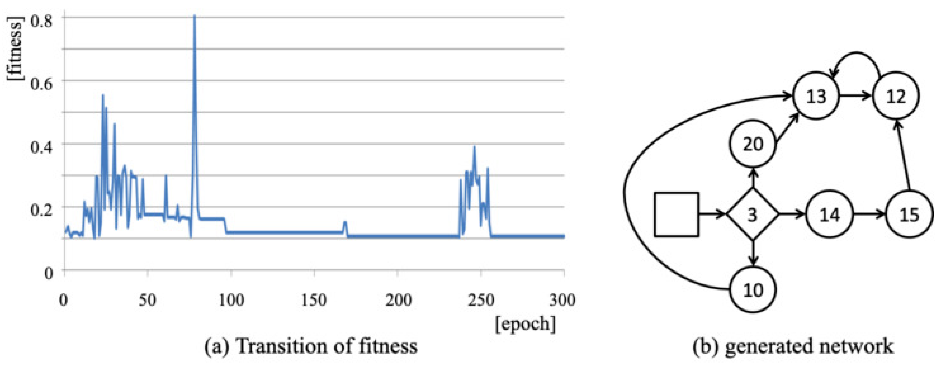
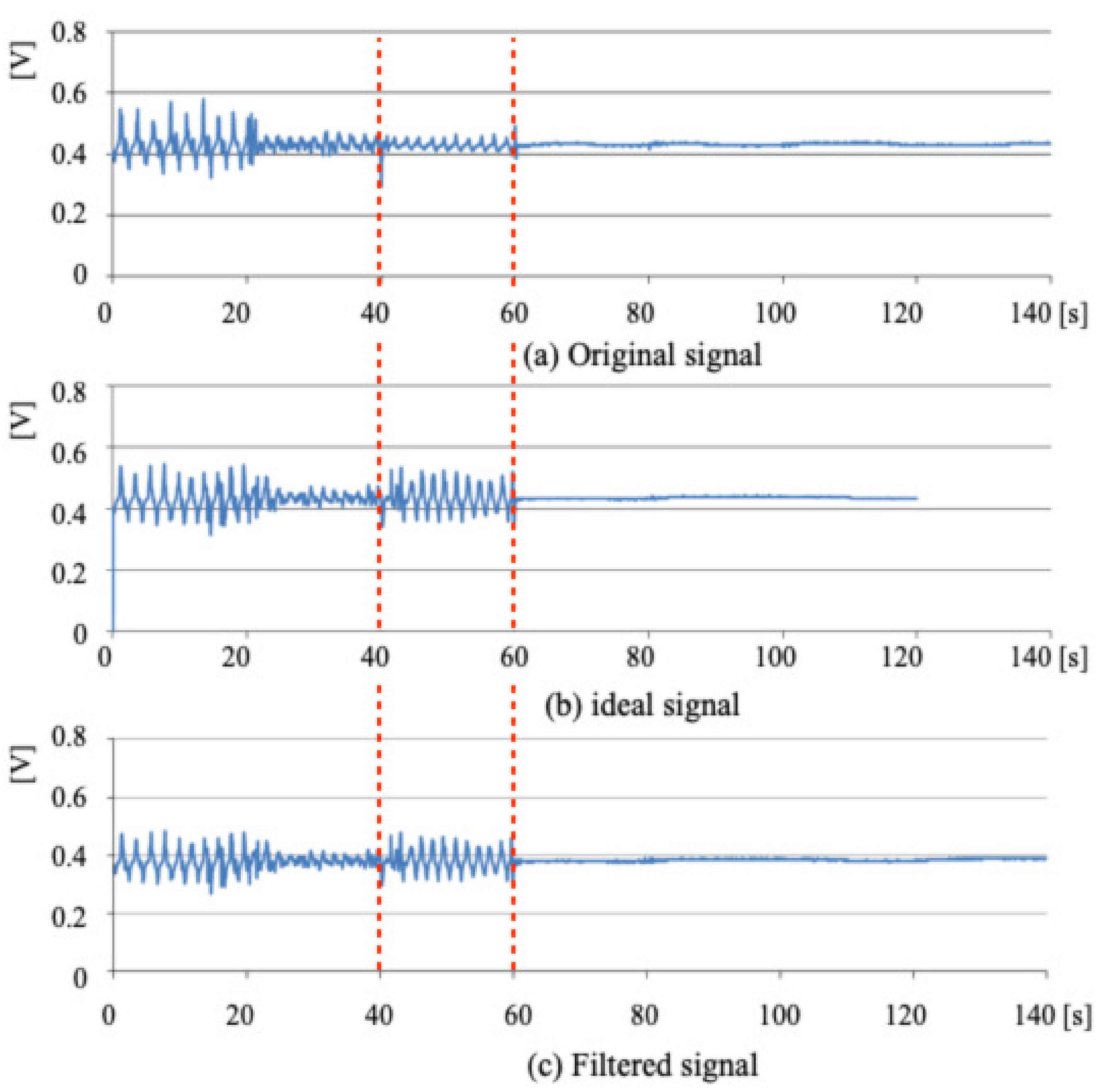
Figure 5 exhibits a generated graph network that comprises one branch node and six processing nodes. Numbers 1–4 and Numbers 5–20 respectively represent branch nodes and processing nodes. Figure 6 depicts the original sensor signals and filtered sensor signals after application of the graph network.
Results demonstrate that the fitness at the 150th epoch was 13.56% higher than that of the 300th epoch. However, the fitness at the 170th epoch and later epochs was almost unchanged until the definitive epoch. Therefore, we infer that the optimal value was reached at approximately the 170th epoch. However, the fitness converged insufficiently. We consider that this convergence is attributable to the wide feature difference between the high-accuracy sensor signals and the low-accuracy sensor signals.
6. Application Experiment
6.1. Setup and Evaluation Criteria
As the evaluation criterion for the results of this experiment, we used recognition accuracy obtained from CPNs as a measure of fitness for optimizing sensor signals. In a report of our earlier study [6], original sensor signals were presented to CPNs to measure the recognition accuracy. This study was conducted to improve the overall system accuracy using GNP as an evolutionary learning approach. From 10 subjects who participated in our earlier study, we selected evaluation targets for this study: six datasets of people for whom the recognition accuracy was the lowest [6]. We used leave-one-out cross-validation to evaluate our method when used along with ML and evolutional learning approaches.
For this experiment, we set as
Intermediate output comprises a binary function as
where is a ground-truth signal at time t.
For this experiment, we infer that our method can correct original signal features, which include noise for negative effects on accuracy, with preservation of salient features for the recognition of bed-leaving behavior patterns. From six datasets, we used the third, fourth and sixth datasets, which had low accuracies.
6.2. Parameters
Table 5 presents parameters that were set based on results of a preliminary experiment. We reduced the maximum generation, individual and mutation to mitigate computational costs for various signal patterns. We used the same setting values for the number of elites, crossover probabilities and mutation probabilities.
6.3. Results and Discussion
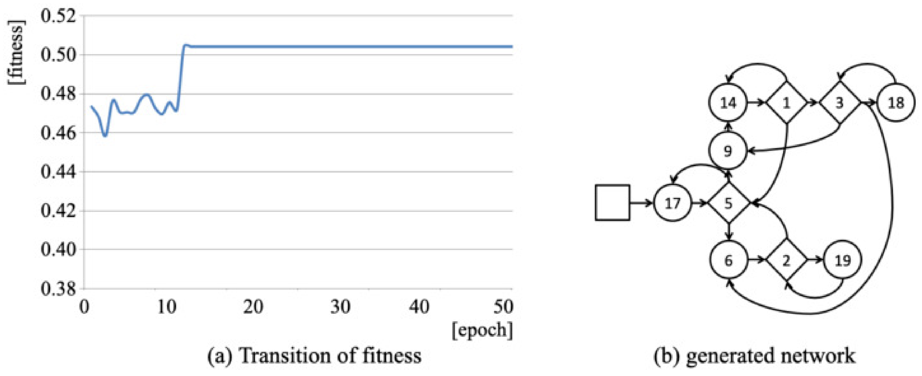
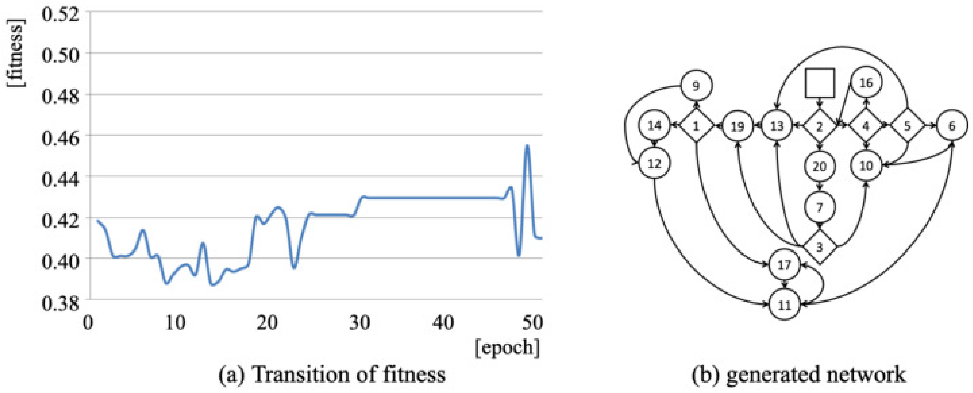
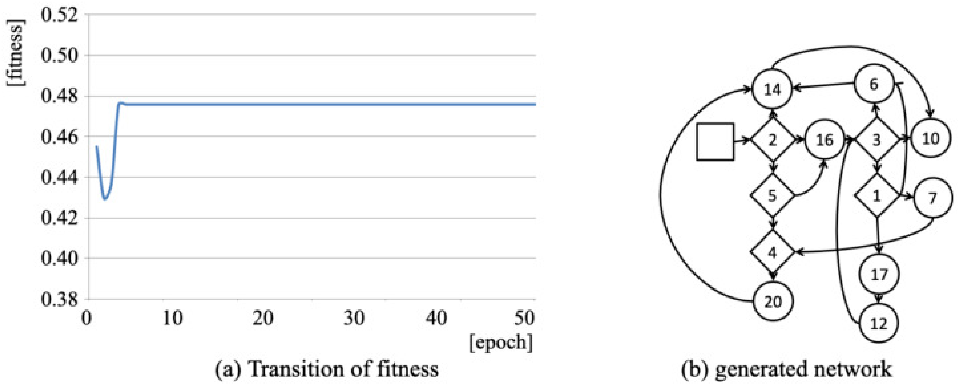
Figure 7a, Figure 8a and Figure 9a respectively portray time series fitness changes of the applied filter sets obtained using GNP for Datasets 4, 5, and 6. In the first half of the transitions up to the tenth epoch, the fitness of our method was lower than the original recognition accuracy. Subsequently, fitness retained high scores with variation. For this experiment, the maximum generation is set to 50 epochs for the iteration of evolutionary learning. Fitness improved slightly in the last half of the transition. Figure 7b, Figure 8b and Figure 9b portray the generated graph networks. Graph networks generated from Datasets 4, 5, and 6 respectively comprise 2, 4, and 4 branch nodes and 8, 9, and 12 processing nodes.
Table 6 presents results obtained from comparison of recognition accuracies from for original signals and filtered signals. As optimization results, the improved accuracies for Datasets 4, 5, and 6 are, respectively, 27.22%, 11.49% and 17.94%. The mean improved accuracy was 18.88% for the three datasets using our method.
7. Detailed Analysis of Parameters and Nodes
This experiment was designed to improve recognition accuracy obtained from based on improved GNP parameters. For parameter optimization, a high burden of computational cost is necessary if all parameters are targeted. We specifically examined two parameters: , which controls the number of mutation; and , which controls the number of crossovers. Moreover, we examined the optimization of filter sets and the node selection calculated from the utilization frequency.
7.1. Parameter of Mutation
We optimized for Datasets 4, 5 and 6. Table 7 presents recognition accuracies with five intervals from 10 to 50. The maximum accuracies of Datasets 4, 5 and 6 were obtained respectively in = 45, 40, and 40. Nevertheless, these results demonstrated, respectively, that the mean improved accuracies for Datasets 4, 5 and 6 were 0.36%, 0.92% and 0.97%. These results addressed that the effects of accuracy for this parameter were tiny when considering improved accuracy.
7.2. Parameter of Crossover
For optimization of , we targeted only Dataset 6 in consideration of the computational costs. Table 8 shows recognition accuracies of 100–400 with 100 intervals. The improved accuracies presented in the third column were increased according to the number of . However, the fourth column shows the sharply increased computational time. Regarding the relation between accuracy and computational cost, we inferred that = 200 is the most suitable for our sensor system.
7.3. Branch Node
Numerous derivatives of branch nodes can be designed. However, we have designed branch nodes manually. Automatic generation of branch nodes has not yet been achieved. For this experiment, we tested the property that the number of derivatives is limited. We added four branched nodes, N21–N24, to the existing branch nodes as shown in Table 9. The definitions of the two formulas are presented below:
Table 10 denotes the top five recognition accuracies of the added branch nodes for Dataset 6. The maximum recognition accuracy of 50.00% was obtained in the additional case of N22 and N24. The recognition accuracy was 4.05% higher than that of 48.05% before the addition.
Table 11 presents the combination of the respective branch nodes and the number of branch nodes used for the application experiment in the previous section. As a utilization tendency, N1 and N2, which compare closed neighbor sensor signals, are used up to one time. By contrast, N3, N4, and N5, which compare wide sensor signals, are used two or three times.
7.4. Processing Node
As with branch nodes, we examined the properties of a limited number of derivatives of processing nodes. For this experiment, we added five processing nodes, N25–N29, to the existing processing nodes as shown in Table 13. Below is the definition.
Table 14 shows the top five recognition accuracies of the added processing nodes for Dataset 6. The maximum recognition accuracy of 50.41% was obtained in the additional case of N25 and N26. The recognition accuracy was 4.91% higher than that before the addition.
Table 15 presents the number of used processing nodes. As a utilization tendency, N7, N8, and N9 process slight signal changes used only one time. In contrast, N15, N18, and N19 process signal changes applied for neighbor sensor signals, used three times. Other nodes were used twice.
Table 16 shows the top five recognition accuracies after changing N7, N8, and N29 to the new processing nodes, as denoted in Table 14. The maximum recognition accuracy of 50.36% was obtained in the case which exchanged N7 and N28, N8 and N26, and N9 and N29. The recognition accuracy was 4.81% higher than that before the exchange.
8. Conclusions
This paper presented a method to generate filters and their optimum sensor signal combination using GNP for improving the recognition accuracy of bed-leaving behavior patterns. We conducted two experiments to demonstrate the basic properties of our method for filtering sensor signals. As the preliminary experiment, we optimized original sensor signals using filters generated using GNP to approximate high-accuracy sensor signals to minimize the fitness-defined difference between them. The experimentally obtained results presented herein reveal that our method provided a filter set that approximates the original signals to ideal signals. For the application experiment, we used the recognition accuracy obtained from CPNs as fitness for evolutional learning. We used three datasets with low accuracy for the evaluation target using leave-one-out cross-validation. Experimentally obtained results reveal that the mean accuracy was improved by 18.88% after applying the generated filters.
Future work shall include an examination of a greater number of target subjects, customizing branch nodes and processing nodes, optimization GNP parameters, verifying the combination with other machine-learning methods, validation of long-term datasets, and the various applications of our method.
Author Contributions
Conceptualization, H.M. and K.S.; methodology, H.M.; software, H.M.; validation, S.N. and K.S.; formal analysis, H.M.; investigation, H.M.; resources, S.N.; data curation, H.M.; writing—original draft preparation, H.M.; writing—review and editing, H.M.; visualization, S.N.; supervision, S.N.; project administration, K.S.; funding acquisition, H.M. All authors have read and agreed to the published version of the manuscript.
Funding
This research was funded by Japan Society for the Promotion of Science (JSPS) KAKENHI Grant Number 17K00384.
Institutional Review Board Statement
Not applicable.
Informed Consent Statement
Not applicable.
Data Availability Statement
Data are available on request.
Conflicts of Interest
The authors declare that they have no conflict of interest. The funders had no role in the design of the study, in the collection, analyses, or interpretation of data, in the writing of the manuscript, or in the decision to publish the results.
Abbreviations
The following abbreviations are used in this manuscript:
| CPN | Counter-propagation network |
| DL | Deep learning |
| EL | Evolutionary learning |
| GA | Genetic algorithm |
| GNP | Genetic network programming |
| GP | genetic programming |
| ML | Machine learning |
| POMDP | Partially observable Markov decision process |
| QoL | Quality of life |
| RFID | Radio-frequency identification device |
| 2D | Two-Dimensional |
References
- Blagosklonny, M.V. Why Human Lifespan is Rapidly Increasing: Solving “Longevity Riddle” with “Revealed-Slow-Aging” Hypothesis. Aging 2010, 2, 177–182. [Google Scholar] [CrossRef] [Green Version]
- Christensen, K.; Doblhammer, G.; Rau, R.; Vaupel, J.W. Aging Populations: The Challenges Ahead. Lancet 2009, 374, 1196–1208. [Google Scholar] [CrossRef] [Green Version]
- Mitadera, Y.; Akazawa, K. Analysis of Incidents Occurring in Long-Term Care Insurance Facilities. Bull. Soc. Med. 2013, 30, 123–130. [Google Scholar]
- Seki, H.; Hori, Y. Detection of Abnormal Action Using Image Sequence for Monitoring System of Aged People. Trans. Inst. Electr. Eng. Jpn. Part D 2002, 122, 1–7. [Google Scholar] [CrossRef] [Green Version]
- Kaji, R.; Hirota, K.; Nishimura, T. Proposal of Detection Method of the State of Fall in Closed Space with RFID Tag System. J. Inf. Process. 2010, 51, 1129–1140. [Google Scholar]
- Madokoro, H.; Nakasho, K.; Shimoi, N.; Woo, H.; Sato, K. Development of Invisible Sensors and a Machine-Learning-Based Recognition System Used for Early Prediction of Discontinuous Bed-Leaving Behavior Patterns. Sensors 2020, 20, 1415. [Google Scholar] [CrossRef] [Green Version]
- Nielsen, R.H. Counterpropagation Networks. Appl. Opt. 1987, 26, 4979–4983. [Google Scholar] [CrossRef]
- Hiramatsu, D.; Madokoro, H.; Sato, K.; Nakasho, K.; Shimoi, N. Automatic Calibration of Bed-Leaving Sensor Signals Based on Genetic Evolutionary Learning. In Proceedings of the 18th International Conference on Control, Automation and Systems, GangWon, Korea, 17–20 October 2018. [Google Scholar]
- Xue, B.; Zhang, M.; Browne, W.N.; Yao, X. A Survey on Evolutionary Computation Approaches to Feature Selection. IEEE Trans. Evol. Comput. 2016, 20, 606–626. [Google Scholar] [CrossRef] [Green Version]
- Song, X.; Yang, Z.; Zhao, J. Preliminary Research of a Medical Sensor Design by Evolution. In Proceedings of the 2008 International Seminar on Future Information Technology and Management Engineering, Leicestershire, UK, 20–20 November 2008; pp. 300–303. [Google Scholar]
- Holland, J.H. Adaptation in Natural and Artificial Systems; University of Michigan Press: Ann Arbor, MI, USA, 1975. [Google Scholar]
- Koza, J.R. Genetic Programming: On the Programming of Computers by Means of Natural Selection; MIT Press: Cambridge, MA, USA, 1992. [Google Scholar]
- Katagiri, H.; Hirasama, K.; Hu, J. Genetic network programming—application to intelligent agents. In Proceedings of the IEEE International Conference on Systems, Man and Cybernetics, Nashville, TN, USA, 8–11 October 2000; pp. 3829–3834. [Google Scholar]
- Katagiri, H.; Hirasama, K.; Hu, J.; Murata, J. Network Structure Oriented Evolutionary Model—Genetic Network Programming—and Its Comparison with Genetic. In Proceedings of the Genetic and Evolutionary Computation Conference, San Francisco, CA, USA, 7–11 July 2001; pp. 219–226. [Google Scholar]
- Hirasawa, K.; Okubo, M.; Katagiri, H.; Hu, J.; Murata, J. Comparison between Genetic Network Programming (GNP) and Genetic Programming (GP). In Proceedings of the Congress on Evolutionary Computation, Seoul, Korea, 27–31 May 2001; pp. 1276–1282. [Google Scholar]
- Katagiri, H.; Hirasawa, K.; Hu, J.; Murata, J.; Kosaka, M. Network Structure Oriented Evolutionary Model: Genetic Network Programming—Its Comparison with Genetic Programming. Trans. Soc. Instrum. Control Eng. 2002, 38, 485–494. [Google Scholar] [CrossRef] [Green Version]
- Goldman, C.V.; Rosenschein, J.S. Emergent Coordination Through the Use of Cooperative State-changing Rules. In Proceedings of the Twelfth National Conference on Artificial Intelligence, Seattle, WA, USA, 31 July–4 August 1994; pp. 408–413. [Google Scholar]
- Mabu, S.; Hirasawa, K.; Hu, J. A Graph-Based Evolutionary Algorithm: Genetic Network Programming (GNP) and Its Extension Using Reinforcement Learning. Evol. Comput. 2007, 15, 369–398. [Google Scholar] [CrossRef]
- Kaelbling, L.P.; Littman, M.L.; Moore, A.W. Reinforcement learning: A survey. J. Artif. Intell. 1996, 4, 237–285. [Google Scholar] [CrossRef] [Green Version]
- Chen, Y.; Mabu, S.; Hirasawa, K.; Hu, J. Genetic network programming with SARSA learning and its application to creating stock trading rules. In Proceedings of the IEEE Congress on Evolutionary Computation, Singapore, 25–28 September 2007; pp. 220–227. [Google Scholar]
- Mabu, S.; Hatakeyama, H.; Thu, M.T.; Hirasawa, K.; Hu, J. Genetic Network Programming with Reinforcement Learning and Its Application to Making Mobile Robot Behavior. IEEJ Trans. EIS 2006, 126, 1009–1015. [Google Scholar] [CrossRef] [Green Version]
- Li, X.; Mabu, S.; Zhou, H.; Shimada, K.; Hirasawa, K. Genetic Network Programming with Estimation of Distribution Algorithms for class association rule mining in traffic prediction. In Proceedings of the IEEE Congress on Evolutionary Computation, Barcelona, Spain, 18–23 July 2010; pp. 1–8. [Google Scholar]
- Li, X.; Mabu, S.; Hirasawa, K. Towards the Maintenance of Population Diversity: A Hybrid Probabilistic Model Building Genetic Network Programming. Trans. Jpn. Soc. Evol. Comput. 2010, 1, 89–101. [Google Scholar]
- Wedashwara, W.; Mabu, S.; Obayashi, M.; Kuremoto, T. Combination of genetic network programming and knapsack problem to support record clustering on distributed databases. Expert Syst. Appl. 2016, 46, 15–23. [Google Scholar] [CrossRef]
- Singh, R.P. Solving 0-1 Knapsack problem using Genetic Algorithms. In Proceedings of the IEEE 3rd International Conference on Communication Software and Networks, Xi’an, China, 27–29 May 2011; pp. 591–595. [Google Scholar]
- Mabu, S.; Chen, C.; Lu, N.; Shimada, K.; Hirasawa, K. An Intrusion-Detection Model Based on Fuzzy Class-Association-Rule Mining Using Genetic Network Programming. IEEE Trans. Syst. Man Cybern. Part C Appl. Rev. 2010, 41, 130–139. [Google Scholar] [CrossRef]
- Zadeh, L.A. Fuzzy Sets. Inf. Control 1965, 8, 338–353. [Google Scholar] [CrossRef] [Green Version]
- Shearer, C. The CRISP-DM Model: The New Blueprint for Data Mining. J. Data Warehous. 2000, 5, 13–22. [Google Scholar]
- Mabu, S.; Higuchi, T.; Kuremoto, T. Semi-Supervised Learning for Class Association Rule Mining Using Genetic Network Programming. IEEJ Trans. Electr. Electron. Eng. 2020, 15, 733–740. [Google Scholar] [CrossRef]
- Henry, A.S.; Daniel, J.I.; Gyuhae, P. A Review of Power Harvesting from Vibration using Piezoelectric Materials. Shock Vib. Dig. 2004, 36, 197–205. [Google Scholar]
- LeCun, Y.; Bengio, Y.; Hinton, G. Deep Learning. Nature 2015, 521, 436. [Google Scholar] [CrossRef] [PubMed]
- Rawat, W.; Wang, Z. Deep Convolutional Neural Networks for Image Classification: A Comprehensive Review. Neural Comput. 2017, 29, 2352–2449. [Google Scholar] [CrossRef]
- Simonyan, K.; Zisserman, A. Very Deep Convolutional Networks for Large-Scale Image Recognition. In Proceedings of the International Conference on Learning Representations, San Diego, CA, USA, 7–9 May 2015. [Google Scholar]
- Guo, Y.; Liu, Y.; Oerlemans, A.; Lao, S.; Wu, S.; Lew, M. Deep Learning for Visual Understanding: A Review. Neurocomputing 2016, 187, 27–48. [Google Scholar] [CrossRef]
- Chong, E.; Han, C.; Park, F.C. Deep Learning Networks for Stock Market Analysis and Prediction: Methodology, Data Representations, and Case Studies. Expert Syst. Appl. 2017, 83, 187–205. [Google Scholar] [CrossRef] [Green Version]
- Xia, X.; Xu, C.; Nan, B. Inception-v3 for Flower Classification. In Proceedings of the 2nd International Conference on Image, Vision and Computing, Chengdu, China, 2–4 June 2017; pp. 783–787. [Google Scholar]
- Chollet, F. Xception: Deep Learning With Depthwise Separable Convolutions. In Proceedings of the IEEE Conference on Computer Vision and Pattern Recognition, Honolulu, HI, USA, 21–26 July 2017; pp. 1251–1258. [Google Scholar]
- He, K.; Zhang, X.; Ren, S.; Sun, J. Deep Residual Learning for Image Recognition. In Proceedings of the IEEE Conference on Computer Vision and Pattern Recognition, Las Vegas, NV, USA, 27–30 June 2016; pp. 770–778. [Google Scholar]
- Xie, S.; Girshick, R.; Dollár, P.; Tu, Z.; He, K. Aggregated Residual Transformations for Deep Neural Networks. In Proceedings of the IEEE Computer Vision and Pattern Recognition, Honolulu, HI, USA, 21–26 July 2017; pp. 5987–5995. [Google Scholar]
- Gao, S.; Cheng, M.; Zhao, K.; Zhang, X.; Yang, M.; Torr, P. Res2Net: A New Multi-Scale Backbone Architecture. IEEE Trans. Pattern Anal. Mach. Intell. 2021, 43, 652–662. [Google Scholar] [CrossRef] [Green Version]
- Beckman, G.H.; Polyzois, D.; Cha, Y.J. Deep Learning-Based Automatic Volumetric Damage Quantification Using Depth Camera. Autom. Constr. 2019, 99, 114–124. [Google Scholar] [CrossRef]
- Carbonaro, N.; Laurino, M.; Arcarisi, L.; Menicucci, D.; Gemignani, A.; Tognetti, A. Textile-Based Pressure Sensing Matrix for In-Bed Monitoring of Subject Sleeping Posture and Breathing Activity. Appl. Sci. 2021, 11, 2552. [Google Scholar] [CrossRef]
- Gaddam, A.; Mukhopadhyay, S.C.; Gupta, G.S. Intelligent Bed Sensor System: Design, Experimentation and Results. In Proceedings of the IEEE Sensors Applications Symposium, Limerick, Ireland, 23–25 February 2010; pp. 220–225. [Google Scholar]
- Motegi, M.; Matsumura, N.; Yamada, T.; Muto, N.; Kanamaru, N.; Shimokura, K.; Abe, K.; Morita, Y.; Katsunishi, K. Analyzing Rising Patterns of Patients to Prevent Bed-related Falls (Second Report). Trans. Jpn. Soc. Health Care Manag. 2011, 12, 25–29. [Google Scholar]
- Liu, J.; Tang, Y.Y. Evolutionary Image Processing. In Proceedings of the IEEE World Congress on Computational Intelligence, Anchorage, AK, USA, 4–9 May 1998; pp. 283–288. [Google Scholar]
Figure 1.
Overall structure of our proposed method including our originally developed sensor.

Figure 2.
Example of genetic network programming (GNP).

Figure 3.
Bed-monitoring sensor system [6].
Figure 3.
Bed-monitoring sensor system [6].

Figure 4.
Output signals in respective sensors.

Figure 5.
Experimentally obtained results of optimizing sensor signals to approximate high-accuracy ideal signals.
Figure 5.
Experimentally obtained results of optimizing sensor signals to approximate high-accuracy ideal signals.

Figure 6.
Original and filtered sensor signals.

Figure 7.
Results of time series fitness changes and generated graph networks for Dataset 4.

Figure 8.
Results of time series fitness changes and generated graph networks for Dataset 5.

Figure 9.
Results of time series fitness changes and generated graph networks for Dataset 6.


Table 1.
Originally designed branch nodes of five types.
| Node Index | First Branch | Second Branch | Third Branch |
|---|---|---|---|
| N1 | |||
| N2 | |||
| N3 | |||
| N4 | |||
| N5 |
Table 2.
Originally designed processing nodes of 15 types.
| Node Number | Formula Index | |||
|---|---|---|---|---|
| N6 | (3) | 0.50 | – | – |
| N7 | (3) | 0.80 | – | – |
| N8 | (3) | 0.90 | – | – |
| N9 | (3) | 1.10 | – | – |
| N10 | (3) | 1.20 | – | – |
| N11 | (3) | 1.50 | – | – |
| N12 | (4) | – | – | – |
| N13 | (5) | – | – | – |
| N14 | (6) | – | – | – |
| N15 | (7) | – | – | – |
| N16 | (8) | – | 0.25 | 0.50 |
| N17 | (8) | – | 0.10 | 0.80 |
| N18 | (9) | – | 0.25 | 0.50 |
| N19 | (9) | – | 0.10 | 0.80 |
| N20 | (10) | – | – | – |
Table 3.
Recognition accuracy in respective datasets. The underlines indicate used datasets.
| Dataset | 1 | 2 | 3 | 4 | 5 | 6 | Mean |
|---|---|---|---|---|---|---|---|
| Accuracy [%] | 43.28 | 43.39 | 41.23 | 39.64 | 40.81 | 40.35 | 41.45 |
Table 4.
Initial setting of GNP parameters.
| Parameters | ||||||||
|---|---|---|---|---|---|---|---|---|
| Setting value | 5 | 15 | 300 | 100 | 60 | 1 | 0.5 | 0.05 |
Table 5.
Setting parameters.
| Parameters | ||||||||
|---|---|---|---|---|---|---|---|---|
| Setting value | 5 | 15 | 50 | 200 | 10 | 1 | 0.5 | 0.05 |
Table 6.
Improved recognition accuracies obtained from .
| Dataset | Before [%] | After [%] | Improvement [%] |
|---|---|---|---|
| 4 | 39.64 | 50.43 | 27.22 |
| 5 | 40.81 | 45.50 | 11.49 |
| 6 | 40.35 | 47.59 | 17.94 |
Table 7.
Optimization experimentally obtained results for .
| Dataset 4 | Dataset 5 | Dataset 6 | |
|---|---|---|---|
| 10 | 50.43 | 45.50 | 17.94 |
| 15 | 50.53 | 45.50 | 48.01 |
| 20 | 50.53 | 45.50 | 47.39 |
| 25 | 50.53 | 45.50 | 48.07 |
| 30 | 50.53 | 46.17 | 48.46 |
| 35 | 50.53 | 45.44 | 48.13 |
| 40 | 50.79 | 46.80 | 49.97 |
| 45 | 51.09 | 46.31 | 46.87 |
| 50 | 50.53 | 46.59 | 47.97 |
| Mean | 50.61 | 45.92 | 48.05 |
Table 8.
Optimization experimentally obtained results for .
| Accuracy [%] | Improvement [%] | Computational time [h] | |
|---|---|---|---|
| 100 | 47.59 | 17.94 | 40.75 |
| 200 | 49.56 | 22.78 | 78.90 |
| 300 | 49.21 | 21.96 | 114.85 |
| 400 | 50.52 | 25.20 | 151.58 |
Table 9.
Optimization experimentally obtained results for .
| Node | Left | Center | RIGHT |
|---|---|---|---|
| N21 | |||
| N22 | |||
| N23 | |||
| N24 |
Table 10.
Top five recognition accuracies of the added branch nodes.
| Ranking | N21 | N22 | N23 | N24 | Accuracy [%] |
|---|---|---|---|---|---|
| 1 | ✓ | ✓ | 50.00 | ||
| 2 | ✓ | 48.83 | |||
| 3 | ✓ | 48.70 | |||
| 4 | ✓ | 48.61 | |||
| 5 | ✓ | ✓ | 48.49 |
Table 11.
Number of branch nodes used.
| N1 | N2 | N3 | N4 | N5 |
|---|---|---|---|---|
| 1 | 1 | 2 | 2 | 3 |
Table 12.
Top five recognition accuracies after changing branch nodes.
| Ranking | N1 | N2 | Accuracy [%] |
|---|---|---|---|
| 1 | same | N24 | 50.50 |
| 2 | N21 | N22 | 49.93 |
| 3 | N23 | same | 48.26 |
| 4 | N21 | same | 47.67 |
| 5 | N23 | N24 | 47.31 |
Table 13.
Additional processing nodes of five types.
| Node | Formula Index | |||
|---|---|---|---|---|
| N25 | (20) | −0.10 | 0.20 | 0.40 |
| N26 | (21) | |||
| N27 | (22) | 0.10 | 0.20 | 0.40 |
| N28 | (23) | 0.05 | 0.15 | 0.60 |
| N29 | (24) | 0.05 | 0.15 | 0.60 |
Table 14.
Top five recognition accuracies of the added processing nodes.
| Ranking | N25 | N26 | N27 | N28 | N29 | Accuracy [%] |
|---|---|---|---|---|---|---|
| 1 | ✓ | ✓ | – | – | – | 50.41 |
| 2 | ✓ | – | – | – | – | 49.26 |
| 3 | ✓ | ✓ | – | ✓ | – | 48.96 |
| 4 | – | ✓ | – | ✓ | ✓ | 48.90 |
| 5 | – | ✓ | – | – | ✓ | 48.54 |
Table 15.
Number of processing nodes used.
| No. of Used Nodes | Index of Nodes |
|---|---|
| 1 | N7, N8, N9 |
| 2 | N6, N10, N11, N12, N13, N14, N16, N17, N20 |
| 3 | N15, N18, N19 |
Table 16.
Top five recognition accuracies after changing processing nodes.
| Ranking | N7 | N8 | N9 | Accuracy [%] |
|---|---|---|---|---|
| 1 | N28 | N26 | N29 | 50.36 |
| 2 | N28 | N26 | – | 50.13 |
| 3 | N25 | N26 | – | 49.71 |
| 4 | N25 | – | – | 49.43 |
| 5 | N25 | N26 | N27 | 48.77 |
Publisher’s Note: MDPI stays neutral with regard to jurisdictional claims in published maps and institutional affiliations. |
© 2021 by the authors. Licensee MDPI, Basel, Switzerland. This article is an open access article distributed under the terms and conditions of the Creative Commons Attribution (CC BY) license (https://creativecommons.org/licenses/by/4.0/).
Share and Cite
MDPI and ACS Style
Madokoro, H.; Nix, S.; Sato, K. Automatic Calibration of Piezoelectric Bed-Leaving Sensor Signals Using Genetic Network Programming Algorithms. Algorithms 2021, 14, 117. https://doi.org/10.3390/a14040117
AMA Style
Madokoro H, Nix S, Sato K. Automatic Calibration of Piezoelectric Bed-Leaving Sensor Signals Using Genetic Network Programming Algorithms. Algorithms. 2021; 14(4):117. https://doi.org/10.3390/a14040117
Chicago/Turabian StyleMadokoro, Hirokazu, Stephanie Nix, and Kazuhito Sato. 2021. "Automatic Calibration of Piezoelectric Bed-Leaving Sensor Signals Using Genetic Network Programming Algorithms" Algorithms 14, no. 4: 117. https://doi.org/10.3390/a14040117
Note that from the first issue of 2016, this journal uses article numbers instead of page numbers. See further details here.