Estimation of Tsunami Bore Forces on a Coastal Bridge Using an Extreme Learning Machine

Abstract

This paper proposes a procedure to estimate tsunami wave forces on coastal bridges through a novel method based on Extreme Learning Machine (ELM) and laboratory experiments. This research included three water depths, ten wave heights, and four bridge models with a variety of girders providing a total of 120 cases. The research was designed and adapted to estimate tsunami bore forces including horizontal force, vertical uplift and overturning moment on a coastal bridge. The experiments were carried out on 1:40 scaled concrete bridge models in a wave flume with dimensions of 24 m × 1.5 m × 2 m. Two six-axis load cells and four pressure sensors were installed to the base plate to measure forces. In the numerical procedure, estimation and prediction results of the ELM model were compared with Genetic Programming (GP) and Artificial Neural Networks (ANNs) models. The experimental results showed an improvement in predictive accuracy, and capability of generalization could be achieved by the ELM approach in comparison with GP and ANN. Moreover, results indicated that the ELM models developed could be used with confidence for further work on formulating novel model predictive strategy for tsunami bore forces on a coastal bridge. The experimental results indicated that the new algorithm could produce good generalization performance in most cases and could learn thousands of times faster than conventional popular learning algorithms. Therefore, it can be conclusively obtained that utilization of ELM is certainly developing as an alternative approach to estimate the tsunami bore forces on a coastal bridge.

1. Introduction

Hundreds of thousands of humans have died in the two most recent giant tsunami tragedies. The Indian Ocean tsunami on 26 December 2004 was among the worst natural tragedies in human history, with human life losses exceeding 300,000 and destructive damage to buildings and infrastructure far beyond the 186 bridges damaged by the tsunami on Sumatra Island [1]. The tragedy of the Great Eastern Japan Tsunami on 11 March 2011 recorded more than 15,883 deaths and more than 300 bridges experiencing significant destruction. Similar to a tsunami disaster, on 29 August 2005 in the United States, Hurricane Katrina caused substantial destruction on the Gulf Coast where more than 1800 people died, huge numbers of buildings were destroyed and 45 bridges suffered damage [2]. 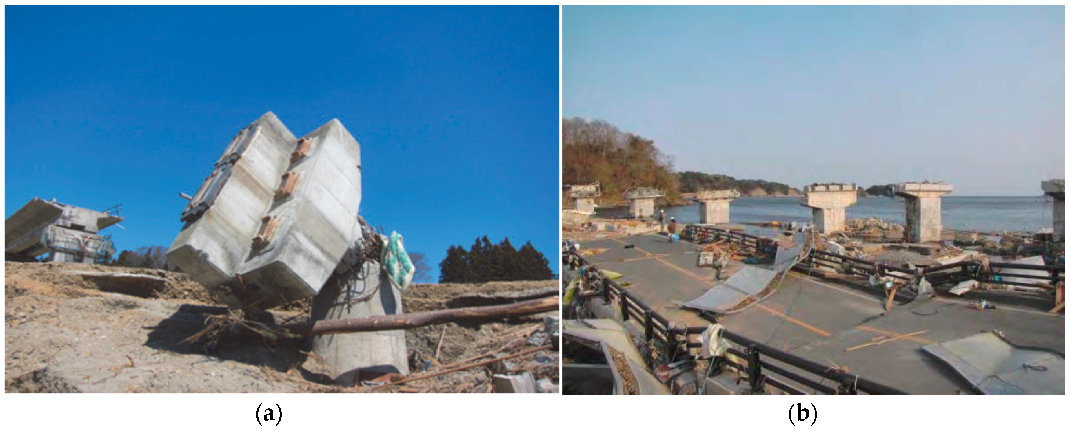Figure 1 illustrates two bridges affected by the Japan Tsunami. It can be concluded that the vital role of a bridge in a high tsunami hazard zone is a reminder to the international scientific community to evaluate, simulate and finally estimate in-depth the tsunami load induced on coastal bridges. A safe design structure for predicting the tsunami load influence on coastal structures requires careful consideration.

Figure 1. (a) Damaged piers of the JR Rail Viaduct at the Tsuya River (photo: S. Dashti); (b) Damages to the deck and piers of Utatsu Bridge (Photo: Kenji Kosa).

Figure 1. (a) Damaged piers of the JR Rail Viaduct at the Tsuya River (photo: S. Dashti); (b) Damages to the deck and piers of Utatsu Bridge (Photo: Kenji Kosa).

Researchers have conducted many valuable experimental studies of tsunami forces on bridges after the huge 2004 Indian Ocean tsunami disaster and 2011 Japan events. A preliminary laboratory examination evaluating the influence of tsunami wave forces on bridges was carried out by Kataoka et al. [3] and continued by other researchers [4,5,6]. Hydraulic experiments were performed to assess tsunami wave loads on bridges and have shown that the impulsive load and uplift force are characteristic of the wave condition. Araki et al. [7] performed an experiment to evaluate the tsunami wave acting on a girder bridge beam. The result indicated that the bridge was influenced by a high amount of horizontal and vertical forces. It was also found that the horizontal force was considerably related to the tsunami height. Thusyanthan and Martinez [8] stated that the highest value of impact pressure in case of a tsunami wave occurred at the bottom of the piers. Shoji et al. [9] conducted hydraulic tests to evaluate breaker bores on the valuation of the drag coefficient. They evaluated the effect of variations of the deck level on a variety of horizontal wave forces on a tsunami wave force. The results stated that the drag coefficient was 1.52 in the condition of surging breaker bores and 1.56 in the case of plunging bores. Lukkunaprasit and Lau [10] and Lau [11] evaluated tsunami loads due to tsunami bore in an inland bridge in two cases of a stand-alone pier and a complete bridge. They stated that the tsunami pressure in the case of a complete pier and deck was 50% higher than in the case of a stand-alone pier model. Hayatdavoodi et al. [12] evaluated the vertical and horizontal load on the bridge deck. The result showed that for shallow water, there was no effect on positive horizontal forces, but there were increases in the negative horizontal forces.

The results of the above studies could not be utilized to estimate the tsunami bore forces on bridges over water. In order to simplify the model fabrication, the piers of bridge models are assumed to be very thin in [3,4,6]. However, in the research [7,9,12], the effect of the tsunami on a complete pier and deck was neglected. This leads to reduced tsunami wave forces on the bridge models in hydraulic experiments. Lukkunaprasit and Lau [10] studied the influence of tsunami bore on a bridge located in a dry bed but did not evaluate the tsunami bore force on coastal bridges over shallow water. Furthermore, all models except for Thusyanthan and Martinez [8] utilized acrylic plates to construct the bridge models. Application of the acrylic plate resulted in decreased measured force by load cells due to reduction of the stiffness, weight of the model and increase in the flexibility of the models [13]. Furthermore, air can be trapped which leads to exaggerated uplift and reduced drag forces. In order to overcome these problems and accurately estimate the bore force on coastal bridge, a more realistic bridge model was applied which utilizes actual materials for both piers and decks. For accurate evaluation, a six-axis load cell was employed in the experiment process.

Analysis of the tsunami bore forces on a coastal bridge require accurate on-line identification. In this article, we motivate and introduce an estimation model of tsunami bore forces including uplift force, drag force and overturning moment on a coastal bridge using a soft computing approach, namely Extreme Learning Machine (ELM). Currently, the application of modern computational approaches in determining the significant challenges and evaluating accurate values has drawn increased attention from scientists in various disciplines, i.e., [14,15,16]. Neural network (NN), as one of the efficient computational methods, has been developed recently in numerous engineering fields. This technique is able to determine challenging nonlinear issues which might be very difficult to eliminate by employing well-known parametric techniques.

Learning time requirement is a main shortcoming of NN techniques. Consequently, an algorithm for a single layer feed forward NN, identified as Extreme Learning Machine (ELM), was presented by Huang et al. [17]. This algorithm is capable of solving problems caused by gradient descent-based algorithms like back propagation which are applied to artificial neural networks (ANNs). ELM methods are capable of reducing the essential time required for learning by a Neural Network. Certainly, it has been verified that by using the ELM, the training procedure becomes quick and it produces robust behavior [17]. Consequently, numerous researches have been conducted associated with utilizing ELM algorithm efficiently for determining problems in various engineering fields [18,19,20,21,22,23,24,25,26].

To summarize, ELM is not only an effective and strong algorithm with a faster learning rate in comparison with classic algorithms such as back-propagation (BP), but it also provides optimum performance. ELM attempts to obtain the lowest training error and also standard of weights. In this study, a predictive model of tsunami bore forces on a coastal bridge was developed using the ELM method. The results indicate that the proposed model can adequately predict the tsunami bore forces including drag force, uplift and overturning moment on a coastal bridge. ELM results were also compared with Genetic Programming (GP) and Artificial Neural Networks (ANNs) results. An attempt is made to establish a correlation between the wave heights, variety of girders in bridges and tsunami bore forces on a coastal bridge. The system should be able to forecast tsunami bore forces on coastal bridges in terms of wave heights.

2. Methodology

The experiments were performed in the Coastal & Offshore Laboratory of University Technology PETRONAS (UTP) and University of Malaya.

2.1. Experiments

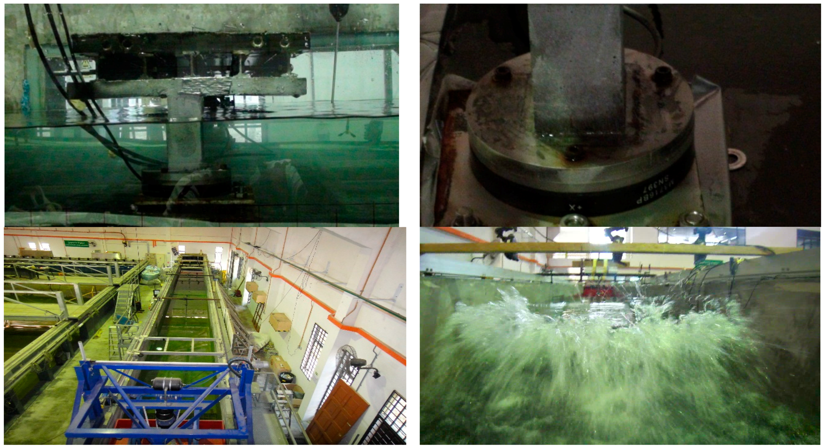
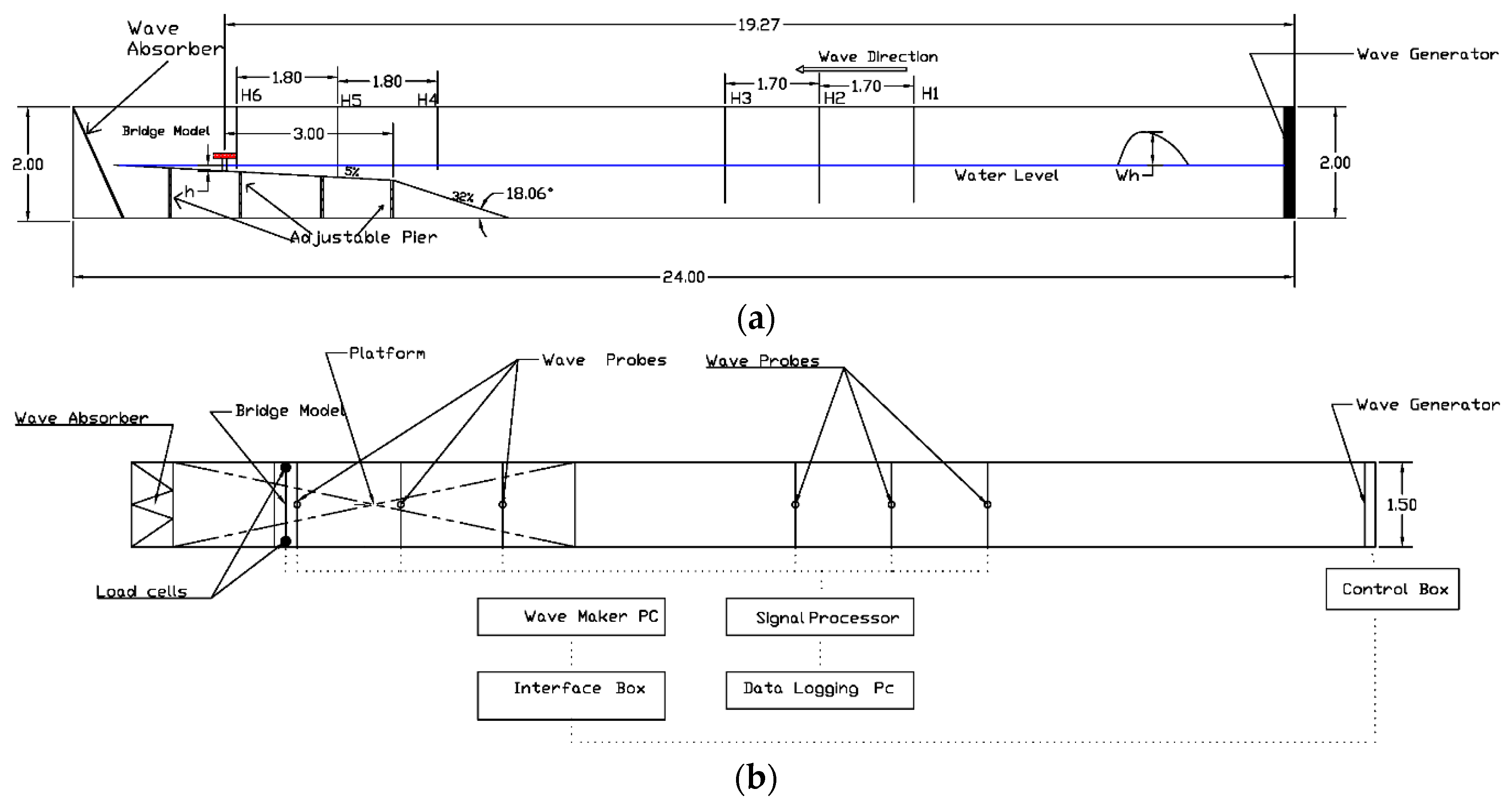
The experiments were carried out in a long wave flume with dimensions of 24 m length × 150 cm wide × 200 cm deep to evaluate and estimate time histories of tsunami bore forces on a bridge model with a variety of wave heights. As illustrated in Figure 2 a piston-type wave generator (pneumatic type) driven by an electric motor controlled by a computer, was applied in this research. The computer automatically performs calculations and determines the necessary force to push the wave-making board by utilizing ocean and wave software supplied by Edinburgh Design Limited. To produce the desired solitary wave height in the wave flume, coded command signals should be employed with the wave computation software in a variety of water depths. For further interpretation of the raw data, the data acquired by WAVELAB (Version 5.0) were stored in the form of data files and analysed using MATLAB (Version 7.2) routines.

A solitary wave was created after the wave generator, as illustrated in Figure 2. The solitary wave moved towards the bridge. On approaching the first slope of the platform, the solitary wave was transformed to an almost vertical wave and broke in the second slope in the still water level, in the form of a breaking wave. Then, the breaking wave changes to a bore in the shallow water. This turbulent bore moved forward and attacked the bridge. The bore then flowed over the platform and contacted the wave absorber at the end of the flume, as illustrated in Figure 2.

Figure 2. Wave flume and model installation in the flume.

Figure 2. Wave flume and model installation in the flume.

2.2. Model

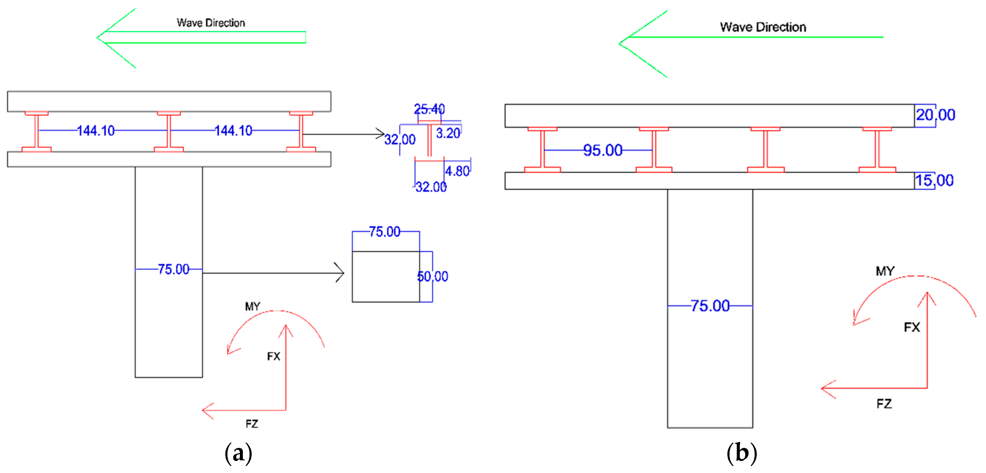
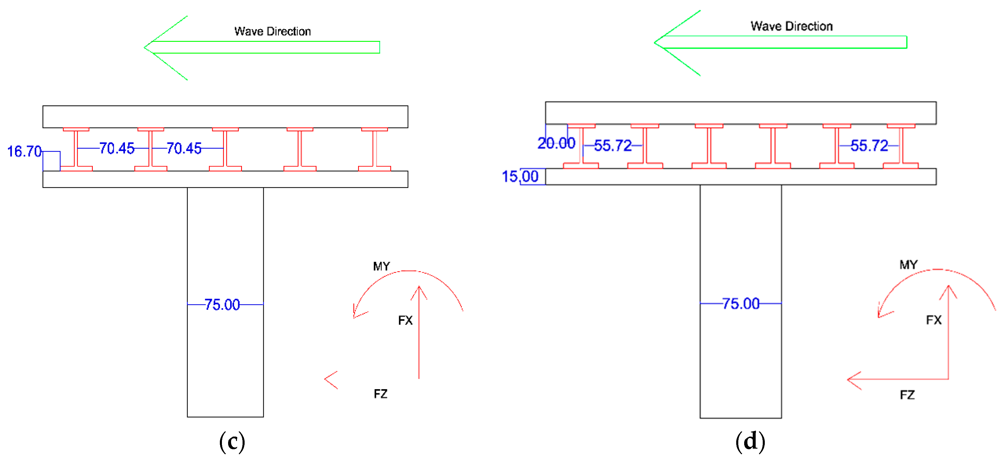
Four bridge models were applied in this research. The bridge model was a typical girder bridge which included a steel plate girder with a concrete deck. The dimensions of the model scaled to 1:40 are given in Figure 3. In these models, three to six girder beams were used. The distance of the girder to the edge of the deck was kept constant for the variety of girder bridges. The distance between girders in three beams (Model A3), four beams (Model A4), five beams (Model A5) and six beams (Model A6) is 144.10 mm, 95.0 mm, 70.45 mm and 55.72 mm, respectively. All beams were fixed with two bolts 90 cm apart from each other and 20 cm from the edge. Two nodes in each side of the beam fixed the beam to the bolts.

Figure 3. Bridge model dimension and the positive direction of drag force, uplift and overturning moment. (a) Model A3; (b) Model A4; (c) Model A5; (d) Model A6.

Figure 3. Bridge model dimension and the positive direction of drag force, uplift and overturning moment. (a) Model A3; (b) Model A4; (c) Model A5; (d) Model A6.

2.3. Setup

In order to measure horizontal drag force, vertical uplift and overturning moment, six-axis load cells were connected to the base plate. The load cells are M3716A units (Sunrise, China) with 135 mm diameter. The capacities of the load cells were FX, FY = 400 N, FZ = 800 N, MX, MY = 40.00 Nm, MZ = 40.00 Nm. Figure 3 illustrates the positive direction of drag force, uplift and overturning moment.

In this research the sampling rate was 1000 Hz. A side view and plan view of the experiment set up is shown in Figure 4. Wave probes in the H1–H6 locations recorded the wave profile as shown in Figure 4. All wave paddles, wave probes and load cells are connected to a data logger named Smart Dynamic Strain Recorder as illustrated in Figure 4b. As illustrated in Figure 4, the platform was designed to characterize the beach profile at the location of the bridge models. The first short steep slope rise of 32% represented the embankment on the proposed beach with a length of 2.2 m and the second slope raised gently by 5% represented the beach slope.

Figure 4. Experimental set up in the flume (a) side view (b) plan view.

Figure 4. Experimental set up in the flume (a) side view (b) plan view.

Three different water depths H_W = 1.0 m, 0.95 m, 0.90 m, were applied in the flume. Ten solitary wave heights were utilized in this research to cover a variety of small to large tsunami wave heights, i.e., $W_h$ = 0.04, 0.8, 0.12, 0.16, 0.20, 0.24, 0.28, 0.32, 0.36, 0.40 m. In order to ensure repeatability and accuracy of the experiment, each hydraulic test was repeated three times and after eliminating the highest and lowest values, the average was recorded and presented in the Results section. The experiments errors were found to be less than 4.5%. The maximum values of vertical, horizontal forces and overturning moment were applied to the results.

2.4. Input and Output Variables

Table 1 and Table 2 illustrate the input and output variables in terms of the definition and obtained values.

Table 1. Input parameters of tsunami bore forces on a coastal bridge.

Inputs	Parameter Description	Parameter Characterization
Input 1	Wh	Wave height
Input 2	T	Velocity

Table 1. Input parameters of tsunami bore forces on a coastal bridge.

Inputs	Parameter Description	Parameter Characterization
Input 1	Wh	Wave height
Input 2	T	Velocity

Table 2. Output parameters.

Output	Parameter Description	Parameter Characterization
Outputs	FX	Uplift
	FZ	Drag force
	MY	Overturning moment

Table 2. Output parameters.

Output	Parameter Description	Parameter Characterization
Outputs	FX	Uplift
	FZ	Drag force
	MY	Overturning moment

2.5. Extreme Learning Machine

Huang, et al. [17] introduced ELM method for Single Layer Feed-forward Neural Network (SLFN) design as a learning algorithm tool [17,27,28]. The ELM algorithm has more effective general ability with faster learning speed. The proposed ELM in most cases has better generalization performance compared to gradient-based learning methods such as back propagation. In addition, ELM picks out the input weights randomly and determines the output weights of SLFN. This is another advantage of the method. ELM does not require excessive human involvement, and is utilized more efficiently than the classic algorithms. Like the unsupervised Artificial Neural Network (ANN), ELM is able to analyse all the network functions, which minimizes human involvement. This method presents an efficient algorithm with various important features such as convenience, prompt learning speed, effective performance, and capability to use most nonlinear stimulation and kernel functions [29].

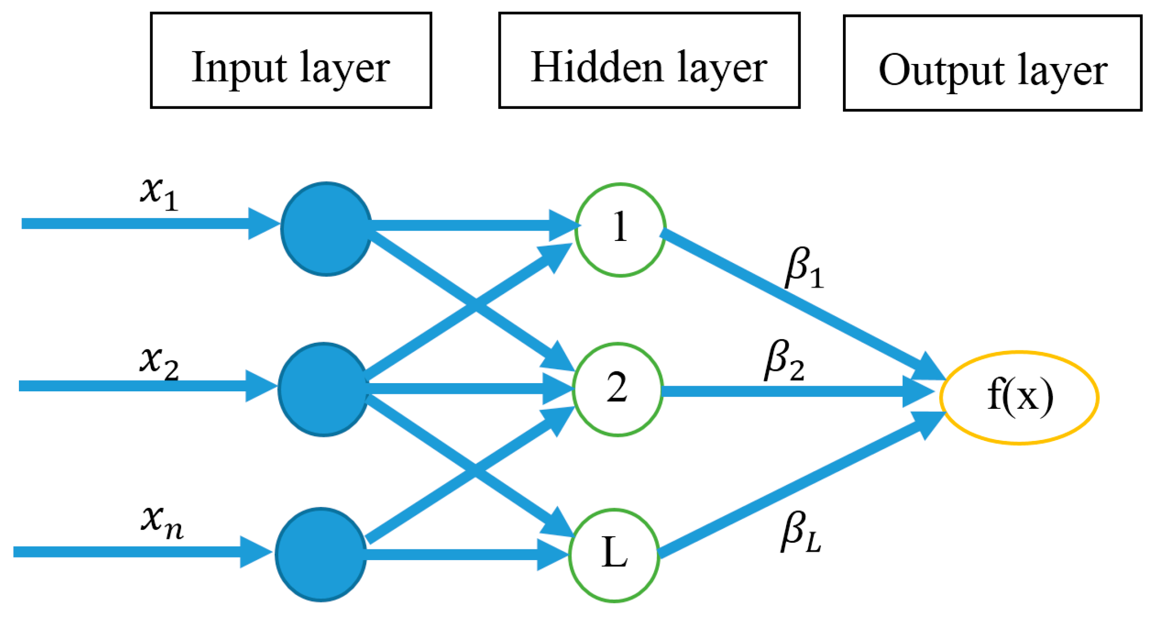
2.5.1. Single Hidden Layer Feed-Forward Neural Network

SLFN is a function with L hidden nodes. It might be characterized by a mathematical equation of SLFN including both additive and radial basis function (RBF) hidden nodes in a unified way given as follows [30,31]:

$$f_L\left(x\right)={\displaystyle \sum }_{i=1}^L{\beta }_{i}G\left(a_i,b_i,x\right),\hspace{1em}\hspace{1em}\hspace{1em}x\in R^n,\hspace{1em}\hspace{1em}\hspace{1em}{a}_i\in R^n$$

(1)

In Equation (1) a_i and b_i represent the learning parameters of hidden nodes. β_i represents the weight connecting the ith hidden node to the output node. $G\left(a_i,b_i,x\right)$ shows the output value of the ith hidden node with respect to the input x. The additive hidden node with the activation function of $g\left(x\right):R\to R$ (e.g., sigmoid and threshold), $G\left(a_i,b_i,x\right)$ is as per [27]:

$$G\left(a_i,b_i,x\right)=g\left(a_i.x+b_i\right),\hspace{1em}\hspace{1em}\hspace{1em}\hspace{1em}{b}_i\in R$$

(2)

where a_i denotes the weight vector which connects the input layer to the ith hidden node. In addition, b_i represented the bias of the ith hidden node. a_i.x represents the inner product of vector a_i and x in Rⁿ. In addition, $G\left(a_i,b_i,x\right)$ might be obtained for RBF hidden node with the activation function $g\left(x\right):R\to R$ (e.g., Gaussian), $G\left(a_i,b_i,x\right)$ as per Huang et al. [27]:

$$G\left(a_i,b_i,x\right)=g\left(b_i\Vert x-a_i\Vert \right),\hspace{1em}\hspace{1em}\hspace{1em}\hspace{1em}{b}_i\in R^{+}$$

(3)

In Equation (3), a_i and b_i represent the centre and impact factor of the ith RBF node, respectively.

R⁺ indicates the set of all positive real values. In this equation, the RBF network describes a particular case of SLFN with RBF nodes in its hidden layer. For N arbitrary distinct samples $\left(x_i,t_i\right)\in R^n\times R^m$, x_i is n × 1 input vector and t_i is m × 1 target vector. In cases where an SLFN with L hidden nodes may estimate the value of N samples with zero error, then it signifies that there exist β_i, a_i and b_i such that [27]:

$$f_L\left(x_j\right)={\displaystyle \sum }_{i=1}^L{\beta }_{i}G\left(a_i,b_i,x_j\right),j=1,\dots .,N.$$

(4)

Equation (4) can be written compactly as:

$$H\beta =T$$

(5)

where:

$$H(\tilde{a},\tilde{b},\tilde{x})={\left[\begin{array}{ccc}G\left(a_1,b_1,x_1\right)& \cdots & G\left(a_L,b_L,x_1\right)\\ & \cdots & \\ \left(a_1,b_1,x_N\right)& \cdots & G\left(a_L,b_L,x_N\right)\end{array}\right]}_{N\times L}$$

(6)

with $\tilde{a}=a_1,\dots ,a_L;\hspace{1em}\tilde{b}=b_1,\dots ,b_L;\hspace{1em}\tilde{x}=x_1,\dots ,x_L$:

$$\beta ={\left[\begin{array}{c}{\beta }_1^T\\ ⋮\\ {\beta }_L^T\end{array}\right]}_{L\times m}\hspace{0.17em}\mathrm{and}\hspace{0.17em}T={\left[\begin{array}{c}{t}_1^T\\ ⋮\\ t_L^T\end{array}\right]}_{L\times m}$$

(7)

In Equations (4)–(7), the H represents the hidden layer output matrix of SLFN that includes the ith column of H, being the ith hidden node’s output with respect to inputs $x_1,\dots ,x_N$. Figure 5 shows the general structure of SLFN ANN structure.

Figure 5. The structure of SLFN.

Figure 5. The structure of SLFN.

2.5.2. Concept of ELM

The ELM technique developed as a SLFN with $L$ hidden neurons has the ability to discover and develop L distinct samples with zero error [20]. However, whenever the number of distinct samples (N) is higher than the number of hidden neurons, ELM method can also randomly allocate variables to the hidden nodes and determine the output weights by pseudo-inverse of H with only a small error ε > 0. a_i and b_i which are hidden node parameters of ELM, should not be tuned throughout learning and may conveniently be allocated with random values. Liang et al. [31] presented the same in the following theorems:

Theorem 1. 

In this theorem Liang et al. [31] presented an SLFN with L additive or RBF hidden nodes as well as an activation function g(x) that is extremely differentiable in every specific R provided. Consequently, for arbitrary L in different input vectors $\left\{x_i|x_i\in R^n,i=1,\dots ,L\right\}$ and ${\left\{\left(a_i,b_i\right)\right\}}_{i=1}^L$, SLFN can randomly be produced by any continuous possibilities assigned. Furthermore, the hidden layer output matrix is invertible with probability one, the hidden layer output matrix H of the SLFN is invertible and $\Vert H\beta -T\Vert =0$, respectively.

Theorem 2. 

In this theorem, Annema et al. [28] provide any small positive value ε > 0 and activation function $g\left(x\right):R\to R$ that is extremely differentiable in every specification; there exists $L\le N$ such that for N arbitrary distinct input vectors $\left\{x_i|x_i\in R^n,i=1,\dots ,L\right\}$ for any ${\left\{\left(a_i,b_i\right)\right\}}_{i=1}^L$ generated randomly according to any continuous possibility distribution provided as $\Vert H_{N\times L}{\beta }_{L\times m}-T_{N\times m}\Vert <\epsilon$ with probability one.

The hidden node variables of ELM should not be tuned during training. Also, Equation (5) due to convenient allocation with arbitrary values, can be transferred to a linear device and the output weights could be determined using the following equation [27]:

$$\beta =H^{+}T$$

(8)

In Equation (8) the Moore-Penrose generalized inverse [32] of the hidden layer output matrix H presented by $H^{+}$ could be estimated by numerous methods, including orthogonal projection, orthogonalization, iterative methods, Singular Value Decomposition (SVD) etc. [32]. The theory of orthogonal projection can be utilized only when $H^{T}T$ is non-singular and $H^{+}={\left(H^{T}T\right)}^{-1}{H}^T$.

There are restrictions in orthogonalization and iterative methods due to the utilization of searching and iterations. While ELM can to be employed in all cases, it can be employed to utilize SVD in calculating the Moore-Penrose generalized inverse of H. Hence, ELM is a batch learning method.

2.6. Artificial Neural Networks

One of the most desired neural network systems is the multilayer feed forward network including a back propagation learning algorithm. This method is extensively utilized in many disciplines such as engineering, science and computing.

The neural network generally includes three sections, i.e., (i) an input section; (ii) an intermediate or hidden section; (iii) an output section. The input vectors consist of $D\in R^n$ and $D={\left(X_1,X_2,\dots ,X_n\right)}^T$, the outputs of $q$ neurons in the hidden section are $Z={\left(Z_1,Z_2,\dots ,Z_n\right)}^T$, and the outputs of the output layer are $Y\in R^m$, $Y={\left(Y_1,Y_2,\dots ,Y_n\right)}^T$, where w_ij and y_j represent the weight and the threshold between the input layer and the hidden layer, respectively, w_jk and y_k assume the outputs of each neuron in a hidden layer and output layer, respectively, as indicated in Equations (9) and (10):

$$Z_j=f\left({\displaystyle \sum }_{i=1}^n{w}_{ij}{X}_i-{\theta }_j\right)$$

(9)

$$Y_k=f\left({\displaystyle \sum }_{j=1}^q{w}_{kj}{Z}_j-{\theta }_k\right)$$

(10)

In Equations (9) and (10), $f$ represents a transfer function, which is the rule for mapping the neuron’s summed input to its output, and utilizes an appropriate option in a device to present a non-linearity into the network design. Generally, the sigmoid function is one of most commonly used functions for monotonic improvement and ranges from zero to one. More details on ANNs can be found in work by several researchers [33,34,35]. The parameters used for the ANN are summarized in Table 3. MATLAB software was used for the ANN simulations.

Table 3. User-defined parameters for ANN.

ANN Parameters
Learning Rate	Momentum	Hidden Node	Number of Iterations	Activation Function
0.2	0.1	3, 6, 10	1000	Continuous Log-Sigmoid Function

Table 3. User-defined parameters for ANN.

ANN Parameters
Learning Rate	Momentum	Hidden Node	Number of Iterations	Activation Function
0.2	0.1	3, 6, 10	1000	Continuous Log-Sigmoid Function

2.7. Genetic Programming

Genetic programming (GP) is an evolutionary algorithm borrowed from the process of evolution occurring in Nature [36] and according to Darwinian theories. It estimates, in symbolic structure, the equation that best expresses the relation of the output to the input variables.

The algorithm assumes an initial random population generated from equation or programs produced from the random combination of input variables, random numbers and functions, i.e., involving operators like multiplication, addition, subtraction, division, square root, log, etc.

This population of potential solutions is then exposed to an evolutionary procedure and the “fitness” (a measure of how well the problem is solved) of the developed programs is assessed. Then, an individual program that represents the higher matching of the data, is selected through the initial population. The individual programs which present better performance, are chosen to exchange part of their data to generate best programs via “crossover” as well as “mutation”. This has simulated the natural world’s reproduction process. However, crossover is exchanging the parts of the best programs with each other and mutation is the random selection of programs to produce a new program. This evolutionary method is continued for following generations and is influenced for obtaining symbolic expressions for describing the data. This leads to scientific interpretation to obtain knowledge about the method [37,38,39]. Table 4 summarizes the parameters used per run of GP. MATLAB software was used for GP simulations.

Table 4. The list of parameters employed in GP modelling.

Parameter	Value
Population size	512
Function set	$+,-,\ast ,/,\surd ,x^2,\ln \left(x\right),e^x,a^x$
Head size	5–9
Chromosomes	20–30
Linking functions	Addition, subtraction, arithmetic, Trigonometric, Multiplication
Number of genes	2–3
Mutation rate	92
One-point recombination rate	0.2
Two-point recombination rate	0.2
Homologue crossover rate	99
Crossover rate	31
Fitness function error type	RMSE
Inversion rate	109
Gene transposition rate	0.1
Gene recombination rate	0.1

Table 4. The list of parameters employed in GP modelling.

Parameter	Value
Population size	512
Function set	$+,-,\ast ,/,\surd ,x^2,\ln \left(x\right),e^x,a^x$
Head size	5–9
Chromosomes	20–30
Linking functions	Addition, subtraction, arithmetic, Trigonometric, Multiplication
Number of genes	2–3
Mutation rate	92
One-point recombination rate	0.2
Two-point recombination rate	0.2
Homologue crossover rate	99
Crossover rate	31
Fitness function error type	RMSE
Inversion rate	109
Gene transposition rate	0.1
Gene recombination rate	0.1

3. Results and Discussion

3.1. Evaluating Accuracy of Proposed Models

Predictive performances of proposed models were presented as Root Means Square Error (RMSE), coefficient of determination (R²) and Pearson coefficient (r). These statistics are defined as follows:

(1) Root Means Square Error (RMSE):

$$RMSE=\sqrt{\frac{{\displaystyle \sum _{i=1}^n{(P_i-O_i)}^2}}{n}}$$

(11)

(2) Pearson correlation coefficient (r):

$$r=\frac{n\left({\displaystyle \sum _{i=1}^n{O}_i\cdot P_i}\right)-\left({\displaystyle \sum _{i=1}^n{O}_i}\right)\cdot \left({\displaystyle \sum _{i=1}^n{P}_i}\right)}{\sqrt{\left(n{\displaystyle \sum _{i=1}^n{O}_i^2}-{\left({\displaystyle \sum _{i=1}^n{O}_i}\right)}^2\right)\cdot \left(n{\displaystyle \sum _{i=1}^n{P_i}^2}-{\left({\displaystyle \sum _{i=1}^n{P}_i}\right)}^2\right)}}$$

(12)

(3) Coefficient of determination (R²):

$$R^2=\frac{{\left[{\displaystyle \sum _{i=1}^n\left(O_i-\overline{O_i}\right)\cdot \left(P_i-\overline{P_i}\right)}\right]}^2}{{\displaystyle \sum _{i=1}^n\left(O_i-\overline{O_i}\right)\cdot {\displaystyle \sum _{i=1}^n\left(P_i-\overline{P_i}\right)}}}$$

(13)

where O_i and P_i are known as the experimental and forecast values of tsunami bore forces on a coastal bridge, respectively, and n is the total number of test data. $\overline{{\text{P}}_{\text{i}}}$ and $\overline{{\text{O}}_{\text{i}}}$ represent average values of P_i and O_i.

3.2. Architecture of Soft Computing Models

The parameters of the ELM, ANN and GP modelling frameworks employed in this study are presented in Table 5. 70% data was used for training and 30% for testing of the models. We didn’t use s validation set since there no indication of overfitting is observed in the models.

Table 5. User-defined parameters for the ELM, ANN and GP models.

ELM		ANN		GP
Number of layers	3	Number of layers	3	-	-
Neurons	Input: 2 Hidden: 3, 6, 10 Output: 1	Neurons	Input: 2 Hidden: 3, 6, 10 Output: 1	Neurons	- - Output: 1
-	-	Number of iteration	1000	Population size	512
Activation function	Sigmoid Function	Activation function	Sigmoid Function	Function set	$+,-,\times ,÷,\surd ,x^2,\ln ,e^x,a^x$
Learning rule	ELM for SLFNs	Learning rule	Back propagation	Head size	5–9
-	-	-	-	Chromosomes	20–30
-	-	-	-	Number of genes	2–3
-	-	-	-	Mutation rate	92
-	-	-	-	Crossover rate	31
-	-	-	-	Inversion rate	109

Table 5. User-defined parameters for the ELM, ANN and GP models.

ELM		ANN		GP
Number of layers	3	Number of layers	3	-	-
Neurons	Input: 2 Hidden: 3, 6, 10 Output: 1	Neurons	Input: 2 Hidden: 3, 6, 10 Output: 1	Neurons	- - Output: 1
-	-	Number of iteration	1000	Population size	512
Activation function	Sigmoid Function	Activation function	Sigmoid Function	Function set	$+,-,\times ,÷,\surd ,x^2,\ln ,e^x,a^x$
Learning rule	ELM for SLFNs	Learning rule	Back propagation	Head size	5–9
-	-	-	-	Chromosomes	20–30
-	-	-	-	Number of genes	2–3
-	-	-	-	Mutation rate	92
-	-	-	-	Crossover rate	31
-	-	-	-	Inversion rate	109

3.3. Performance Evaluation of Proposed ELM Model

In this section, performance results of ELM tsunami bore forces on a coastal bridge predictive model are reported. Figure 6a, Figure 7a and Figure 8a present the accuracy of developed ELM tsunami bore forces on a coastal bridge predictive model, while Figure 6b, Figure 7b, Figure 8b, Figure 6c, Figure 7c and Figure 8c present the accuracy of developed GP and ANN tsunami bore forces on a coastal bridge predictive model, respectively. The results demonstrated that the majority of the points fall along the prediction line of ELM model. Therefore, there is very good agreement between measured values and prediction values for ELM method. This consideration may be verified with the quite high value for the coefficient of determination. As results show, the variety of overestimated or underestimated values produced in ELM method are limited. Accordingly, it is evident that the predicted values have a high level of accuracy.

Figure 6. Scatter plots of actual and predicted values of tsunami bore force FX on a coastal bridge using (a) ELM, (b) GP and (c) ANN method.

Figure 6. Scatter plots of actual and predicted values of tsunami bore force FX on a coastal bridge using (a) ELM, (b) GP and (c) ANN method.

Figure 7. Scatter plots of actual and predicted values of tsunami bore force FZ on a coastal bridge using (a) ELM, (b) GP and (c) ANN method.

Figure 7. Scatter plots of actual and predicted values of tsunami bore force FZ on a coastal bridge using (a) ELM, (b) GP and (c) ANN method.

Figure 8. Scatter plots of actual and predicted values of tsunami bore moment MX on a coastal bridge using (a) ELM, (b) GP and (c) ANN method.

Figure 8. Scatter plots of actual and predicted values of tsunami bore moment MX on a coastal bridge using (a) ELM, (b) GP and (c) ANN method.

4. Performance Comparison of ELM, ANN and GP

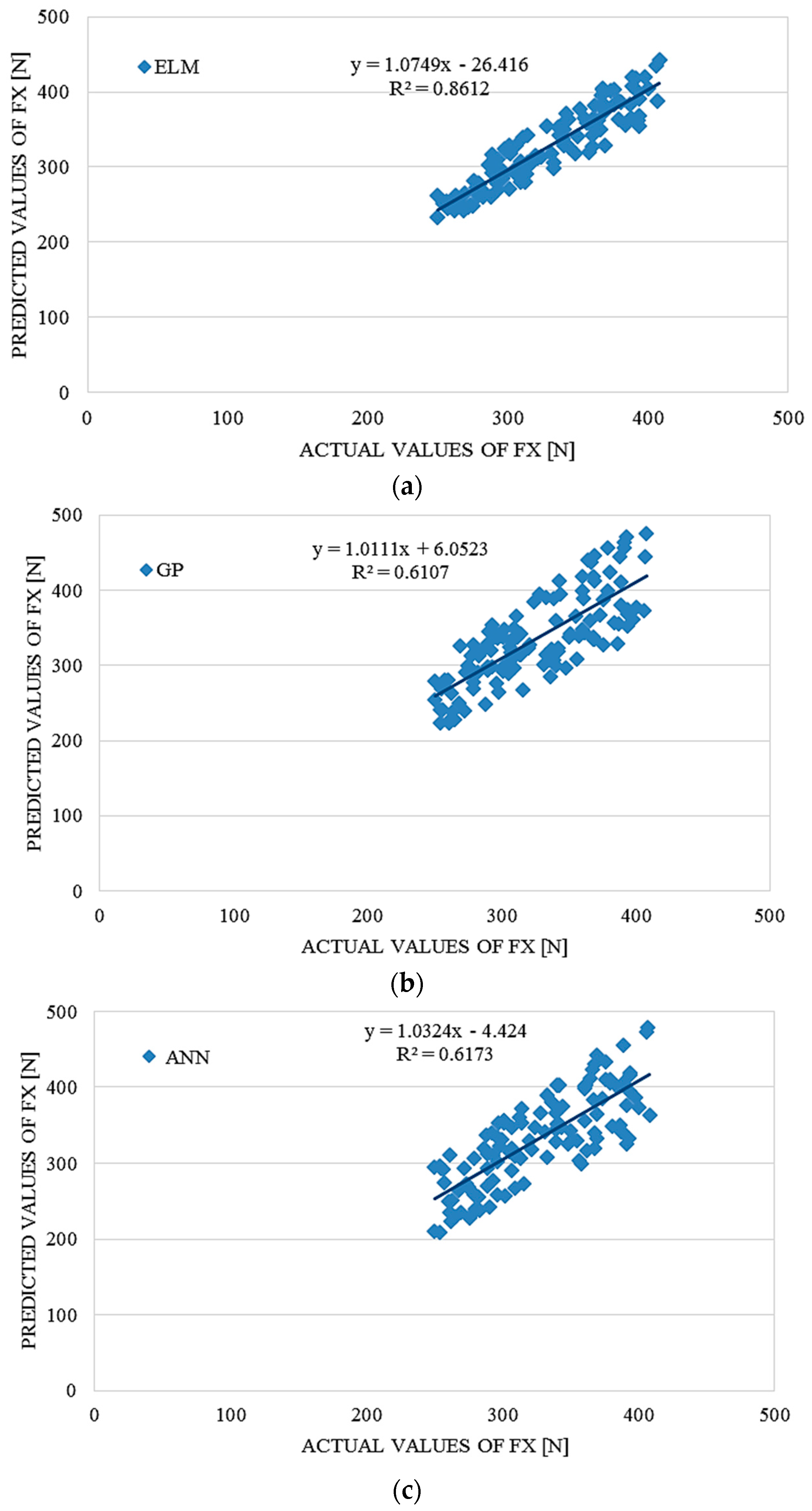
To evaluate the accuracy and advantages of the proposed ELM approach, the ELM model’s prediction accuracy was compared with prediction accuracy of GP and ANN methods, which were used as a benchmark. In order to compare, conventional error statistical indicators, RMSE, R² and r, were applied. Table 6 and Table 7 summarize the prediction accuracy results for test data sets since training error is not a credible indicator for the prediction potential of the particular model. This results present average results after many repetitions and many iterations in order to fins optimal structures of the models. The average computation time for the ELM modelling was around 310 seconds using a PC with an Intel Core Duo CPU E7600 @3.06 GHz and 2 GB RAM. The average computation time for the ANN and GP modelling using the same PC with the same performances was 424 and 446 s, respectively. For the ELM modelling, MATLAB software was used.

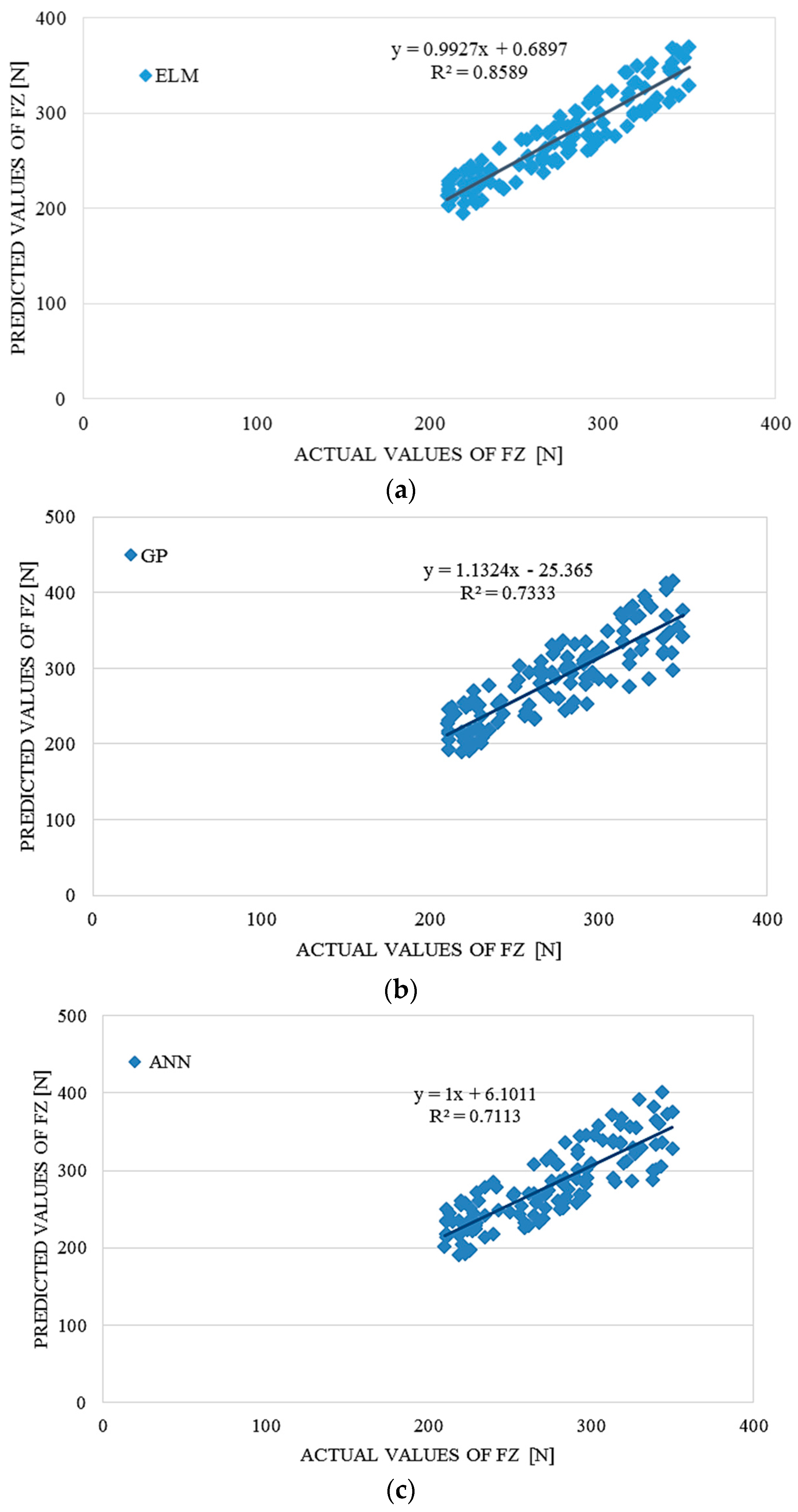
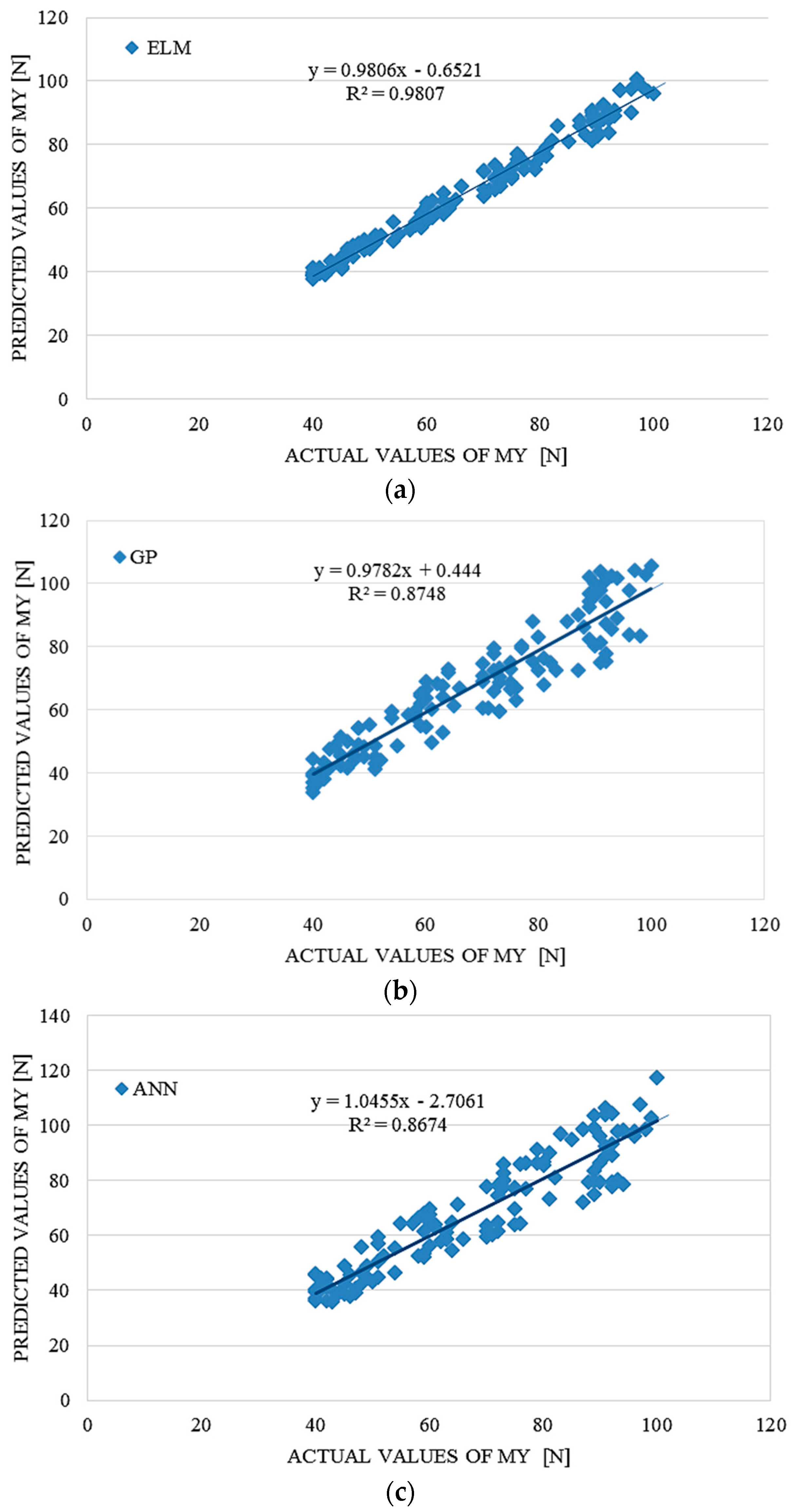
The ELM model outperformed the GP and ANN models according to the results in Table 6, Table 7 and Table 8, providing significantly better results than the benchmark models. On the basis of the RMSE analysis in comparison with ANN and GP, it could also be concluded that the proposed ELM outperformed the results obtained with benchmark models.

Table 6. Comparative performance statistics of the ELM, ANN and GP tsunami bore force FX on a coastal bridge predictive model.

ELM			ANN			GP
RMSE	R2	r	RMSE	R2	r	RMSE	R2	r
19.32297	0.8612	0.92799	36.39317	0.6173	0.78570	36.13951	0.6107	0.78150

Table 6. Comparative performance statistics of the ELM, ANN and GP tsunami bore force FX on a coastal bridge predictive model.

ELM			ANN			GP
RMSE	R2	r	RMSE	R2	r	RMSE	R2	r
19.32297	0.8612	0.92799	36.39317	0.6173	0.78570	36.13951	0.6107	0.78150

Table 7. Comparative performance statistics of the ELM, ANN and GP tsunami bore force FZ on a coastal bridge predictive model.

ELM			ANN			GP
RMSE	R2	r	RMSE	R2	r	RMSE	R2	r
17.00278	0.8589	0.92676	26.92342	0.7113	0.84336	28.85849	0.7333	0.85631

Table 7. Comparative performance statistics of the ELM, ANN and GP tsunami bore force FZ on a coastal bridge predictive model.

ELM			ANN			GP
RMSE	R2	r	RMSE	R2	r	RMSE	R2	r
17.00278	0.8589	0.92676	26.92342	0.7113	0.84336	28.85849	0.7333	0.85631

Table 8. Comparative performance statistics of the ELM, ANN and GP tsunami bore moment MY on a coastal bridge predictive model.

ELM			ANN			GP
RMSE	R2	r	RMSE	R2	r	RMSE	R2	r
2.53381	0.9807	0.99030	7.52946	0.8674	0.93532	6.81423	0.8748	0.93132

Table 8. Comparative performance statistics of the ELM, ANN and GP tsunami bore moment MY on a coastal bridge predictive model.

ELM			ANN			GP
RMSE	R2	r	RMSE	R2	r	RMSE	R2	r
2.53381	0.9807	0.99030	7.52946	0.8674	0.93532	6.81423	0.8748	0.93132

5. Conclusions

This research used out a systematic experimental and numerical method to create a ELM predictive model of tsunami bore forces on a coastal bridge. The experimental validation was performed in a 24 m tsunami flume on 1/40 scale girder bridge with various numbers of girders and wave heights. The tsunami bore forces consisting of horizontal, uplift forces and overturning moment, were measured in various cases. A comparison of the ELM method with GP and ANN was conducted in order to evaluate the forecast accuracy and reliability. Accuracy results, measured in terms of RMSE, r and R², indicate that the ELM predictions are superior to those of GP and ANN. Additionally, the results reveal the robustness of the method.

The produced ELM method provides numerous interesting and extraordinary capabilities which indicate the significant advantages of this method in comparison with conventional well-known gradient-based learning algorithms for feed-forward neural networks. Significantly higher accuracy and much faster learning speed could be achieved bu using ELM when compared with the classic feed-forward network learning algorithms, for instance the back-propagation (BP) algorithm. Furthermore, in contrast to traditional learning algorithms, the ELM algorithm is designed to produce the lowest training error and norm of weights.