Investigating the Physics of Tokamak Global Stability with Interpretable Machine Learning Tools

Featured Application

Machine-learning-based techniques have been applied to disruption prediction in Tokamaks and, by symbolic regression via genetic programming, physically meaningful equations have been extracted from the machine learning models, helping to investigate disruption physics and to transfer present-day knowledge to future devices.

Abstract

The inadequacies of basic physics models for disruption prediction have induced the community to increasingly rely on data mining tools. In the last decade, it has been shown how machine learning predictors can achieve a much better performance than those obtained with manually identified thresholds or empirical descriptions of the plasma stability limits. The main criticisms of these techniques focus therefore on two different but interrelated issues: poor “physics fidelity” and limited interpretability. Insufficient “physics fidelity” refers to the fact that the mathematical models of most data mining tools do not reflect the physics of the underlying phenomena. Moreover, they implement a black box approach to learning, which results in very poor interpretability of their outputs. To overcome or at least mitigate these limitations, a general methodology has been devised and tested, with the objective of combining the predictive capability of machine learning tools with the expression of the operational boundary in terms of traditional equations more suited to understanding the underlying physics. The proposed approach relies on the application of machine learning classifiers (such as Support Vector Machines or Classification Trees) and Symbolic Regression via Genetic Programming directly to experimental databases. The results are very encouraging. The obtained equations of the boundary between the safe and disruptive regions of the operational space present almost the same performance as the machine learning classifiers, based on completely independent learning techniques. Moreover, these models possess significantly better predictive power than traditional representations, such as the Hugill or the beta limit. More importantly, they are realistic and intuitive mathematical formulas, which are well suited to supporting theoretical understanding and to benchmarking empirical models. They can also be deployed easily and efficiently in real-time feedback systems.

1. Disruptions in Tokamaks: An Operational Perspective

Many systems, both natural and man-made, can be stable for long times and may look quite resilient but, in reality, they are not immune to catastrophic collapse. Some of the failures leading to collapse are relatively straightforward to interpret and do not seem worthy of particular attention; indeed, they can be consistently avoided once the proper precautions are put in place. Other collapses are due to very subtle and extremely difficult to predict causes. Earthquakes, and in general failures due to atmospheric phenomena, belong to the second category. In recent years, various efforts have been devoted to developing mathematical tools more appropriate to investigating and predicting these catastrophic and typically rare phenomena. Machine learning tools, of the type described in this paper, constitute an additional family in the arsenal of mathematical approaches, which can be used to study catastrophic events [1].

In the field of Magnetic Confinement Nuclear Fusion, disruptions are the most striking example of catastrophic failures difficult to predict. Therefore, they are one of the most severe problems to be faced by the Tokamak magnetic configuration in the attempt to design and operate commercial reactors. Disruptions are also a not negligible difficulty for the present largest devices, such as JET, and indeed they pose a not irrelevant constraint to high current operation. Moreover, JET disruptivity with the new ITER-like Wall (ILW) remains too high for the next generation of machines, since at low q₉₅ the percentage of disruptions can easily exceed 25%. To put this value in perspective, on DEMO even, one unmitigated disruption could severely damage the reactor [2].

Since they constitute a potential serious hazard to the integrity of Tokamak devices, disruptions are the subject of extensive studies at present. From the perspective of ultimate remedial actions that can be undertaken, various methods of mitigation are being investigated, particularly massive gas injection and shatter pellets. A complementary approach to manage the problem of disruptions is based on avoidance, i.e., on the sufficiently early detection of problems in the discharges and the consequent implementation of corrective actions to avoid the abrupt termination of the plasma.

From an operational perspective, robust and reliable prediction methods are a prerequisite to any mitigation or avoidance strategy. Unfortunately, the theoretical understanding of the causes of disruptions is not sufficient to guarantee reliable forecasts, particularly on the time scales required for avoidance. Lacking solid and detailed theoretical models of disruptions, the development of an operation-based description of Tokamak plasmas aimed at determining the boundaries of the safe space, in terms of physically controllable quantities, has been attempted. One of such empirical descriptions of plasma stability is the so-called Hugill diagram, which combines the low q and density limits [3]. The low q limit is expressed in terms of 1/q₉₅, where q₉₅ is the safety factor at 95% of the plasma radius. The density limit is typically based on the Murakami factor n_eR/B_T, where n_e is the mean electron density, R the plasma major radius and B_T the toroidal field. For a large JET database with the ILW (see Section 4), the Hugill diagram is reported in Figure 1. Unfortunately, such a plot has very poor predictive and interpretative capability, since the disruptive and safe regions overlap almost completely in this space.

Similar considerations apply to another popular diagram, used to investigate the so-called beta limit [3]. The parameter β is typically used to quantify the level of the plasma pressure compared to the magnetic pressure. It is therefore natural to expect that pressure-driven instabilities could limit the level of β achievable in a certain configuration. This limit is typically represented as a function of the parameter I_*l_i/(aB_T), where I is the plasma current, l_i the internal inductance and a the minor radius. The β-limit plot for various campaigns of JET with the ILW is reported in Figure 2. Again, inspection of the plot reveals that, in this space, it is practically impossible to separate the disruptive from the safe operational regions. Therefore, from a practical point of view, these representations have poor predictive and interpretative capability, at least for JET with the ILW.

The inadequacies of theoretical and empirical models of disruptions have motivated the development of data driven predictors. From this perspective, several machine learning methods have been developed. They cover a wide range of techniques from Fuzzy logic classifiers to neural networks [4,5,6,7,8,9,10,11,12,13,14,15]. In recent years, a new predictor, Advanced Predictor Of DISruptions (APODIS), based on Support Vector Machines (SVMs), has been deployed in the JET real-time network and has performed very satisfactorily in terms of both success rate and false alarms, in a long series of campaigns without any need for retraining [7]. Manifold learning tools, such as Self Organising Maps and Generative Topographic Maps have provided very good results also for the task of automatically determining the disruption type, many tens of ms in advance of the beginning of the current quench [16,17]. Some of these classifiers have implemented a new metric based on the Geodesic Distance on Gaussian manifolds [18]. Even if these data-driven tools are producing quite impressive results, their main problem, particularly from the perspective of next step devices, is the number of examples required for training. In large machines such as ITER, it would be practically impossible to collect hundreds of disruptions to train the most satisfactorily performing machine learning tools such as APODIS. In the last couple of years, therefore, many efforts have been devoted to the developments of parsimonious data-driven techniques that can provide a good success rate of prediction after a few tens of disruptions and even after the first disruption [19,20,21]. Their future application is very promising, particularly if coupled with new methods to avoid disruptions [22,23,24] and to model the stability boundary [25].

The main remaining issues, with these advanced Machine Learning (ML) tools, are now their physics fidelity and the interpretability of their results. They have shown the potential to learn very efficiently from few examples, but they operate in such a way that their models do not necessarily reflect the dynamics behind the phenomenon. Since the resulting models are also very difficult to interpret, in the present format machine learning tools cannot really contribute to the interpretation of the physics behind disruptions.

To increase the contribution of machine learning tools to the investigation of the physics of global stability in Tokamaks, a new methodology has been devised to reconcile the knowledge acquired by the ML techniques with mathematical expressions of a more traditional form, in terms of interpretable formulas, which can be used both as a guide for analysis developments and as a benchmark of theoretical models. This approach combines the predictive performance and the knowledge discovery capability of ML tools with the necessity to formulate the results in such a realistic way that they can be related to physical theories capable of extrapolation to larger devices.

The methodology, to derive physically meaningful models from machine learning tools, consists of the following steps:

• Training the machine learning tools for classification, i.e., to discriminate between disruptive and non-disruptive examples;
• Identifying a sufficient number of points on the boundary between safe and disruptive regions of the operational space on the basis of the models derived by the machine learning tools;
• Deploying Symbolic Regression via Genetic Programming to express the equation of the boundary in a physically meaningful form, using the points identified in the previous step;
• Converge on the final model with the help of the Pareto Frontier and non-linear fitting.

This procedure for the identification of the disruptive boundary in Tokamaks is an original development proposed here for the first time to the community (a preliminary version of the methodology was introduced in a conference contribution to a completely different audience [26]). In the work presented in this paper, the knowledge discovery tasks rely on Support Vector Machines (SVMs) and ensembles of Classification and Regression Trees (CARTs), whose mathematical background is briefly summarised in the next section. This choice is driven by the need to provide a fully general and sound methodology. In this respect, it should be remembered that SVM and CART ensembles are completely different approaches to learning and give absolutely different types of mathematical models. They are also positioned at quite opposite extremes of the machine learning techniques (see next section): kernel and rule-based methods, respectively. Therefore, the more than satisfactory results reported in this work prove not only the generality of the approach but also increase the confidence in the methodology and conclusions.

SVMs are particularly recommended by their good generalisation properties, which guarantee very high success rates, provided the training set is adequate. In addition to traditional Support Vector Machines, the proposed method is also adapted to a probabilistic version of SVM, to show in general how the approach can be particularised for machine learning tools, which provide outputs of this nature. Ensembles of classifiers are a more recent solution, which has been very successful in the development of adaptive predictors [5,27,28,29,30]. Their basic units, decision trees, are a typical example of rule-based classifiers and constitute a completely different approach to machine learning. The flexibility provided by the ensembles constitutes a very good complement to kernel techniques, such as SVM.

To formulate the output of SVM and ensembles of CART in a physically realistic and interpretable way, extensive use is made of Symbolic Regression via Genetic programming; these techniques are therefore covered in Section 2. The actual combination of the various tools, to provide the equation of the boundary between two regions of the operational space, is covered in Section 3. A representative example of the systematic series of numerical tests, performed to prove the potential of the proposed techniques, is reported in Appendix A. JET database with the ITER-like Wall is introduced in Section 4 and the results, in terms of equations for the boundary between the disrupting and non-disruptive regions of the operational space, are the subject of Section 5 and Section 6. More specifically, Section 5 describes an exploratory application and Section 6 a confirmatory one. The lines of future investigations are covered in the following Section 7, together with a final discussion.

2. Classifiers and Symbolic Regression via Genetic Programming

In this Section, a short overview of the machine learning tools developed, to provide interpretable equations of the disruption boundary, are summarised. Since, in their general form, they are well-known techniques, already deployed in the field of thermonuclear fusion, only a bird’s eye view is provided in this section. The reader interested in the details will have to make recourse to the references.

2.1. Support Vector Machines

Support Vector Machines (SVMs) are very powerful techniques with various desirable properties for scientific applications [30,31,32,33,34]. Probably their main use is as binary classifiers, and it is in this capacity that they have been deployed in the present work. Conceptually, the specificity of SVM consists of mapping the inputs to be classified into a high dimensional space. This projection is achieved with already available mathematical operators called kernels, which in the most general versions of the classifiers are fully non-linear. The mapping into these high dimensional, or even infinite dimensional, spaces allows a better separation between the classes, which the SVM achieves by constructing a hyperplane in terms of the features selected by the user. The best hyperplane, the one which minimises the risk of misclassification, is derived by maximising the margins between the closest points of the two classes, called Support Vectors (SVs), and the hyperplane itself. The rule to classify a feature vector x as disruptive or non-disruptive depends on the sign of this distance to the hyperplane [35].

Given the high generalisation capability that they achieve by implementing the margins, SVMs are very powerful tools and have performed extremely well in the case of disruption prediction, as demonstrated in real time for example by APODIS. Their hyperplane can therefore be considered a particularly good approximation of the boundary between the disruptive and not disruptive regions of the operational space. On the other hand, their mathematical representation of the boundary bears no resemblance to the underlying dynamics of the physical phenomenon under investigation and is extremely non-intuitive. In the case of disruptions on JET, the equation of the hyperplane can easily comprise hundreds of support vectors and, consequently, the equation of the hyperplane presents an equal number of addends.

Recently, various approaches to derive probabilities from SVMs have emerged and have provided interesting results. The availability of classifiers, which can output a probability, would be extremely useful in most applications. Since traditional SVMs provide only a distance to a hyperplane, their standard version requires a reformulation of their models, so that a probability can be associated to their predictions. A popular alternative takes advantage of the Bayes rule and this is the approach adopted for the present work [34].

2.2. Classification and Regression Trees

The confirmatory technology of classifiers investigated is Classification and Regression Trees (CARTs). CARTs are rule-based machine learning tools, designed to derive the classification “rules”, for the solution of a given problem, directly from data. They operate by recursively partitioning the feature space and building a decision tree. At each partition, they select the feature and its value, which provide the best separation of the two classes, in the sense of minimising the impurity of each child node (the purity of a node reaches a higher level the greater the number of its members, which belong to a single class). At each partition, the CART then identifies the best rule to fit the data [35,36]. The final model therefore consists of a series of if…then rules that can be represented as trees. In terms of representational power, CART trees have the same expressive power as propositional logic.

The CART technology is well consolidated and its positive characteristics, such as flexibility and interpretability, are well understood. The routines for their implementation are also well established and very efficient. On the other hand, these machine learning tools tend to show a severe lack of robustness. Indeed, they can be excessively influenced by the details of the training set; therefore, slightly different examples in the training set can result in quite different sets of rules. Once deployed, these different classifiers can therefore produce excessively different outputs.

A consolidated solution to this unfortunate tendency is constituted by pooling many CART classifiers into so called ensembles [34,35]. These ensembles are basically groups of not highly successful CART classifiers that, thanks to their computational efficiency, can be pooled together with suitable techniques to obtain much higher performance. To this end, the outputs of the individual classifiers are combined with appropriate decision functions, to provide the final response [34,35].

The CART ensembles can also associate a probability to their outputs, in full analogy to the case of the probabilistic SVM [34,35]. On the other hand, even this simple overview reveals that CART ensembles and SVM are completely independent mathematical techniques; their combination can therefore significantly increase the confidence in the obtained results.

2.3. Symbolic Regression via Genetic Programming

As briefly discussed in Section 1, the subject of this paper is the application of Symbolic Regression (SR) via Genetic Programming (GP) to identifying a physically meaningful equation for the boundary between safe and disruptive regions of the operational space. The main advantages of the proposed approach consist of: (a) flexibility in implementing the most appropriate assumptions about the mathematical form of the boundary; (b) allowing one to express the equations of the boundary in mathematical forms, which reflect the physics of disruptions and permit comparison with theory. The other specific characteristic of the proposed methodology resides in its capability to identify the most suitable mathematical expressions, for the boundary between safe and disruptive regions of the operational space, directly from the experimental data. So, no prior information about the mathematical form of the boundary is required because the developed tools allow extracting the most suited expression directly from the database.

The technique is based on generating a high number of formulas, built combining basis functions covering a sufficiently wide spectrum to describe the phenomenon to be studied, and on determining which ones better fit the data. Such a task is achieved efficiently by Genetic Programming.

Genetic Programming is a collective name comprising a series of mathematical techniques, in which programmes are represented as some sort of genes and then adapted to solving specific optimisation problems by evolutionary computational methods [36,37,38,39]. Genetic Programs (GPs) are meant to emulate the natural selection of the genotype in living organisms. GPs manipulate a population of individuals, which are mathematical expressions in our case. Each individual constitutes a potential equation for the boundary between the safe and disruptive regions of the operational space in the application presented in this paper. The quality of each individual, with respect to the available data, is assessed by means of a utility function that, in this context, is normally referred to as Fitness Function (FF). The FF is basically a metric determining how good an individual is in solving the problem at hand, given the data. The individuals of the current generation, with a better value of this metric, are granted a higher probability to pass their genes to descendants. In other words, the probability that the genes of an individual are inherited by the following generation is linked to its performance in terms of the FF.

Once the final structure of the candidate models has been agreed upon, typically with the method of the Pareto Frontier, the parameters of the model, obtained with SR via GP, are typically refined with appropriate nonlinear fitting routines [40]. In addition to improving their values, this step allows associating confidence intervals to the parameters of the models. All the details about the methodology described in this Section can be found in [40,41,42].

3. Identification of the Boundary Equation between Safe and Disruptive Regions of the Operational Space

This section introduces the innovative part of the work presented in this paper: the mathematical procedure, to obtain the equation of the boundary between disruptive and non-disruptive operational regions, by applying symbolic regression to the outputs of machine learning tools, namely SVM and ensembles of CART classifiers (Section 3.1 and Section 3.2, respectively). Numerical examples, to elucidate the details, and to prove that the approach works for problems of the same level of complexity as the experimental databases investigated in the rest of the paper, are reported in Appendix A. Some considerations about the computational requirements of the techniques are also mentioned (Section 3.3).

3.1. Combining SVM and Symbolic Regression

As mentioned, the developed methodology consists mainly of two parts. First, points on the SVM separating hypersurface are generated and, secondly, they are fitted with symbolic regression. In the case of probabilistic SVM, the first task is banal. Indeed, the available tools allow deriving equal-probability surfaces. It is therefore sufficient to extract the points that correspond to the chosen level of probability. These points can then be fitted with SR via GP to obtain the required equation.

The situation is a bit more involved in the case of traditional SVM, which provides a distance to the separating hypersurface and not directly points on the hypersurface. The solution for this more complicated case is reported in the following for completeness sake and for the benefit of systems using the traditional version of the SVM [26]. A remark about the nomenclature of the SVM technique is probably in place at this point. Since the objective of the proposed methodology consists of finding an equation for the boundary in the original space, and not in the transformed space, from now on the boundary will be referred to as a hypersurface (and not a hyperplane, which is the mathematical solution of the SVM in the transformed space).

As mentioned, the interpretation of the models, provided by the SVM, requires the reformulation of their boundary equation in more physically meaningful equations. To this end, a sufficient number of points, belonging to the hypersurface separating the two classes, must be derived, so that they can be regressed with SR via GP. For this task, first a mesh is built, with resolution equal or better than the error bars of the measurements, selected as the features for the inputs to the SVM. More grid points and a better refined mesh can improve numerical convergence and stability; therefore, the total number of grid points can be set based on computational considerations. On the other hand, suitable criteria are available for selecting more efficiently the number of intervals in different directions. The first one consists of allocating more intervals along the direction of stronger curvature. The second alternative is that of allocating a higher number of mesh points in the direction of the dependent variable, to be sure that the selected points are close enough to the real hypersurface.

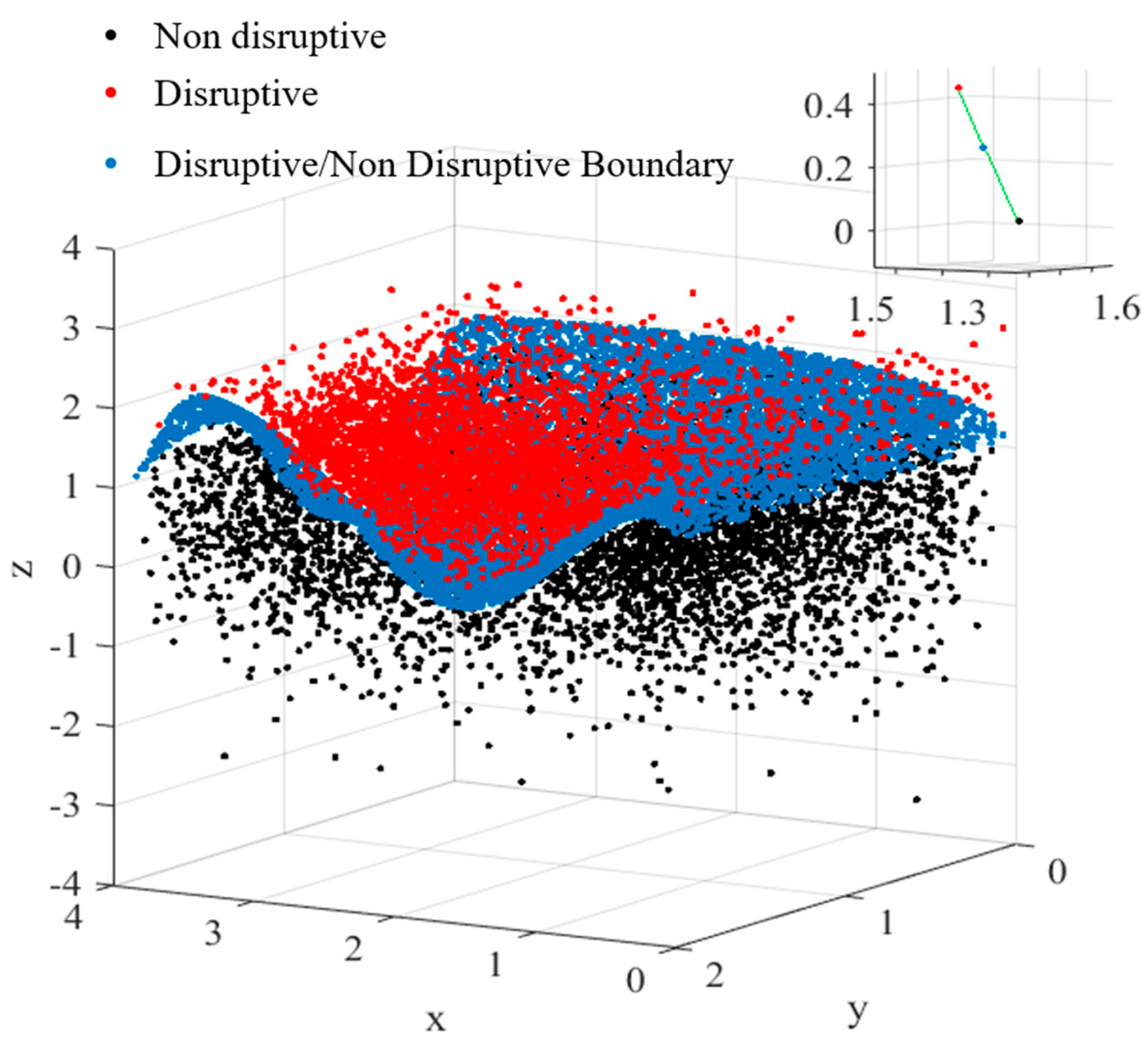
Once the mesh has been built, the algorithm proceeds by selecting first the Support Vectors (SVs) on one side of the hypersurface, let us say the positive side, to fix the ideas. From these starting points, the routines move towards the support vectors on the other side, one point on the grid at the time. At each step, the already trained SVM is interrogated to determine the distance of the current point to the hypersurface. If the SVM confirms that the distance is positive, the process is iterated, since the current point remains on the same side of the hypersurface. When the distance of a new grid point becomes negative, the two points with different signs are on opposite sides of the boundary between the two classes. They can therefore be considered as belonging to the hypersurface. Indeed, by construction of the mesh, two subsequent points, for which Equation (1) changes sign, are within a distance from the hypersurface, which is within the error bars of the measurements. For all practical purposes, the points, identified with the procedure just described, are therefore close enough to the boundary to be considered on it. This method to obtain SVM hypersurface points, for a numerical example using synthetic data, is illustrated pictorially in Figure 3.

After checking that a sufficient number of points near the hypersurface have been collected, the equation of the hypersurface itself can be derived by deploying symbolic regression via genetic programming. For assessing the quality of the final models, various alternatives can be implemented. A natural first choice is based on the statistical indicators described [40,41,42]. Another very important step, to prove the quality of the obtained equations, consists of testing their success rate of classification. These two types of checks implicitly assure also that an appropriate number of points on the hypersurface have been retained.

3.2. Combining CART Ensembles and Symbolic Regression

As is well known, CART ensembles are also supervised classifiers, which after training attribute each example to a class. CART ensembles can also associate a probability to their output, by suitably mediating the outputs of the individual trees. The extraction of the points required for SR via GP is therefore immediate as for the case of probabilistic SVM. On the other hand, in the case of the ensembles, in addition to the choice of the threshold, the user can adjust additional parameters. For example, a possible refinement consists of excluding the output of the trees, which have proved to perform significantly worse than the average of the others. On the other hand, to improve interpretability, simply a few of the best trees can be selected if they provide sufficient performances. Other alternatives are the increase in the number of individual trees or multiple runs, for example, with different realisations of the noise. All these procedures are of course meant to improve the reliability and the interpretability of the final probabilistic output and they also grant additional flexibility to adjust the performances and align them with the objectives of the investigation.

3.3. Computational Requirements

To provide some basic information about the computational resources required for the deployment of the proposed techniques, the run time to train the SVM or the CART ensembles is not a major issue, since it is typically orders of magnitude shorter than the other calculations and it is therefore negligible compared to the following steps of the procedure. Coming to building the grid, required when working with traditional SVM, with a Windows 64-bit operating system computer with eight cores and 24 gigabyte of RAM (an Intel Xeon E5520, 2.27 GHz, 2 processors), finding the hypersurface points on a grid of 16⁴ × 51 takes of the order of 3 h. The GP calculation, including the building of the Pareto Frontier, is typically about one order of magnitude longer. Therefore, the computationally more demanding task is SR via GP step. In this respect, one should consider that genetic programs, of the type deployed in this application, are easy to parallelise. Consequently, very significant reductions in computational time can be expected if a more sophisticated version of the routines is implemented.

4. Database of JET with the ITER-Like Wall

In building the database, the intentional disruptions and those in which the control system had activated the massive gas injection have been excluded from the training. Only times when the plasma current exceeds 750 kA have been considered. All the signals used as input features have been resampled at 1kH frequency. Since on JET 10, ms is the shortest interval to implement reliable mitigation strategies, alarms, launched less than the10 ms from the beginning of the current quench, are considered tardy. Early alarms are those triggered more than 2.5 s before the beginning of the current quench; this is a conservative assumption because on JET with the ILW the main cause of disruptions is impurity accumulation, which takes place on time scales even longer that the 3 s.

In more detail, campaigns C29 to C31 have been analysed. Various considerations have motivated this choice. First, the investigated campaigns are at the beginning of the operation of JET with the ITER-like Wall. The results are therefore more relevant for the next generation of devices and also simulate the beginning of the operation of a new machine. Moreover, in these first campaigns with the ILW, very little use was made of the fast valve to mitigate the effects of the disruptions with massive gas injection. The JET control system therefore did not interfere much with the natural evolution of the discharges, which is the situation of interest for the subject of analyses of the present work.

The database has been divided into two parts. The data of C29 and C30 have been analysed with the aim of providing interpretable models. The examples of the campaign C31 have then been kept in reserve to form a test set; so the models have been derived from the examples of C29–C30 and have then been used to classify the completely new data of C31.

After suitable cleaning and validation of the databae, campaigns C29–C30 provided overall 187 disruptive and 1020 non-disruptive shots, unless differently specified (in some analyses at the end of the paper, the need to consider additional variables, which are not always available, will require a slight reduction in the statistical basis). Campaign C31 provided a total of 590 examples: 154 disruptions and 436 safe discharges. The operational space covered by the database is summarised graphically in Figure 4. As can be seen from the reported plots, the set of discharges considered is representative of JET operation with the ILW; therefore, the same quality of the results is to be expected also if the methodology is applied to future campaigns.

The set of signals, considered as potential inputs to the predictors, includes: the vacuum toroidal magnetic field B, the plasma current I, the edge density n, the amplitude of the locked mode LM, the safety factor at 95% of the plasma radius q95 and the amplitude of the internal inductance li. The locked mode amplitude is estimated from the measurements of the saddle coils. The internal inductance is obtained from the Shafranov integrals calculated on the plasma last closed magnetic surface. The safety factor q95 is an output of EFIT, the main equilibrium reconstruction code used at JET.

5. A Data-Driven Model for JET with the ILW

To illustrate the potential of the proposed methodology, in this section the task of extracting a mathematical model directly from the data is assessed. The case discussed is an example, for which the “a priori” knowledge about the problem is kept to a minimum. For the sake of simplicity and linearity of explanation, only the probabilistic versions of SVM and CART ensembles are discussed but the same results and considerations are valid also for the other versions of the tools.

The SVM and CART ensembles are applied to the database without any bias and, in particular, various possible input variables have been tested, to converge on the two providing the best results. The objective of this example is to show how the technique proposed can be used to obtain a practical, easily interpretable, and implementable formula in two dimensions. The issues related to building models of higher dimensionality, giving the data available, are discussed in the next section.

JET campaigns C29–C30 with the ILW have been used to train the SVM and the CART ensembles. In the case of the disruptive discharges, the 12 ms interval before the beginning of the current quench are divided into four subintervals of 3 ms each, and the averages of these three subintervals are the features. For the safe discharges, an interval of 40 ms on the flat top is divided in four 10 ms ranges and the averages over those subintervals are the features. In the first exploratory phase, the SVM and the CART ensembles have been trained with a wide set of global quantities as inputs, to identify the two features providing the best performance. In agreement with previous investigations reported in the literature, the locked mode and the internal inductance amplitudes turn out to be the most informative signals. Indeed, the classifiers, using these inputs, achieve by far the best results. This fact confirms various past studies, which have shown quite convincingly that these two quantities are quite essential in predicting the occurrence of disruptions at least for mitigation purposes [5,6,7,10,11,18,19,20,21,27,28,29].

Using the LM and l_i amplitudes, the posterior probabilities have then been calculated as indicated in Section 2. The outputs of the ML classifiers have been investigated for a whole range of threshold probabilities. It turns out that the probability value, which provides the best performance for both classifiers, is around 80% for both techniques; this has been confirmed by a systematic scan of the classifiers developed for the present study. Therefore, the model trained with this threshold is the one whose results have been reported in the paper. It is worth mentioning that, for the interval (50%, 80%) of threshold probability, all the models give very similar results [27]. So, the choice of the threshold is not too critical for the purpose of the present paper, the identification of a manageable formula to describe the boundary between safe and disruptive regions of the operational space.

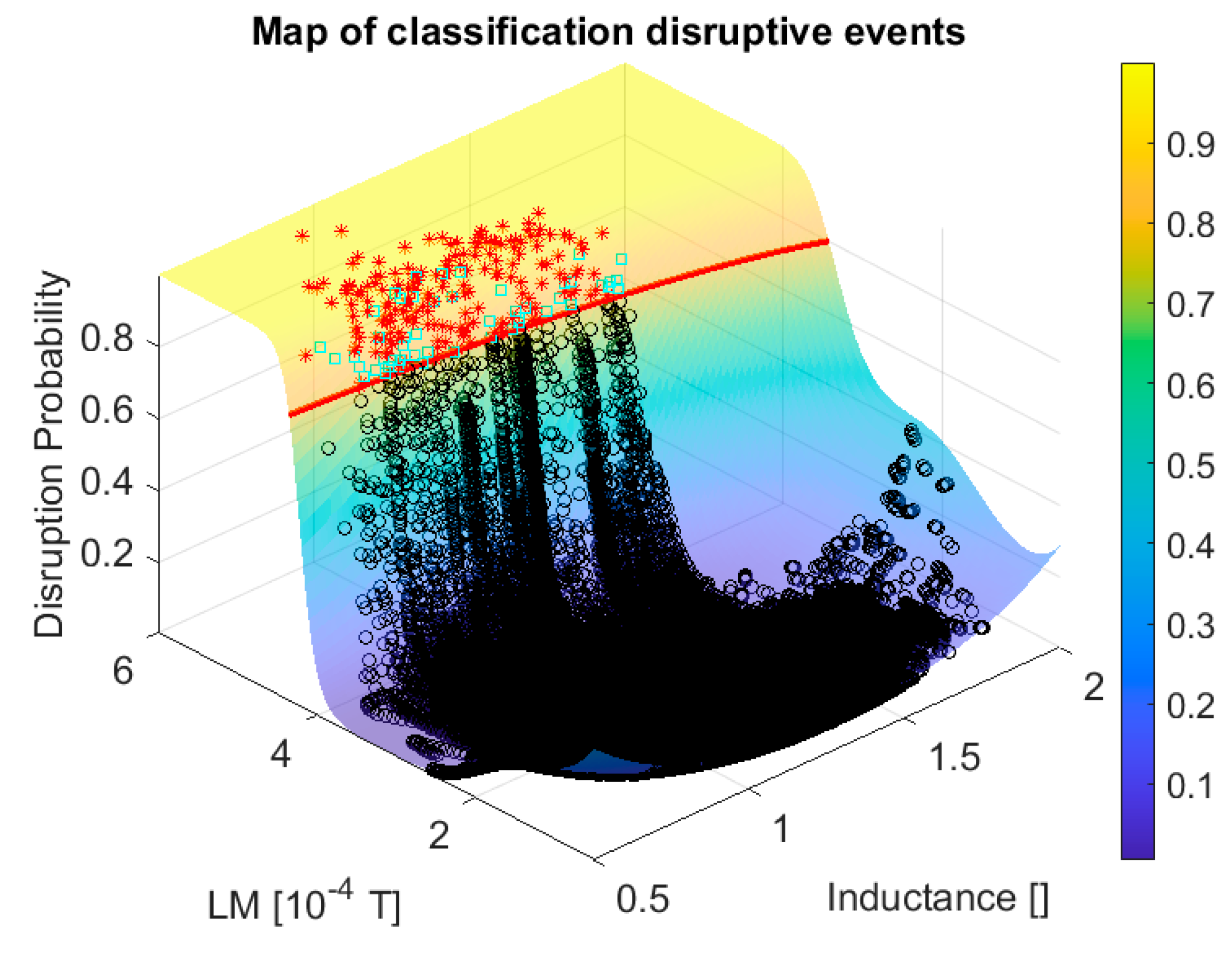
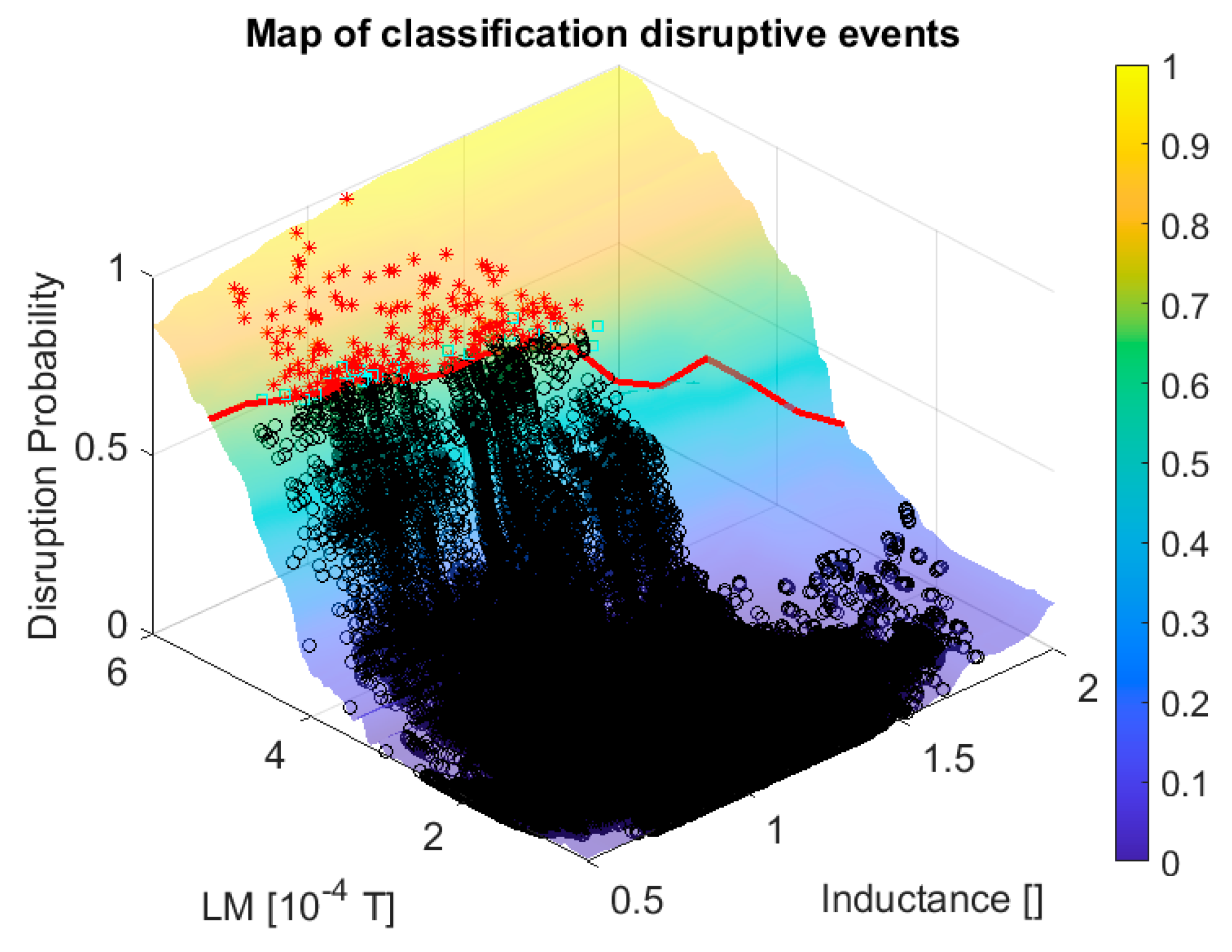
The curve level plots of the posterior probability are reported in Figure 5 for the SVM and in Figure 6 for the CART ensemble. The safe and disruptive regions are well separated in the plane of the locked mode and internal inductance. This clear discrimination is confirmed by the results in terms of success rate and false alarms reported in the first two rows of

Table 1. The figures of merit obtained using SVM (threshold probability 80%) and Equation (1) for campaigns C29–C30.

Method	Success Rate	Missed	Early	Tardy	False	Mean (ms)	Std (ms)
SVM	97.9% (183/187)	0% (0/187)	0% (0/187)	2.1% (4/187)	2.8% (29/1020)	335	344
CART Ensemble	94.7% (177/187)	0% (2/187)	0% (0/187)	4.3% (8/187)	2.3% (23/1020)	336	345
SR via GP Equation (1)	97.9% (183/187)	0% (0/187)	0% (0/187)	2.1% (4/187)	2.7% (28/1020)	336	345

, from which it is easy to appreciate the extremely good performance of both probabilistic classifiers. In this, as in all the other tables, the last two columns report the mean and standard deviation of the interval elapsing between the time of the alarm and the disruption, i.e., the beginning of the current quench.

The methodology, described in Section 3, has then been applied to the SVM model and the CART ensembles, to obtain a manageable equation of the boundary. After the analysis performed with the Pareto Frontier, the following equation has been retained as a reasonable compromise between complexity and accuracy:

$$LM\left(l_i\right)=a_0\exp \left(a_1{l}_i^{a_2}\right)$$

(1)

where LM is the amplitude of the locked mode expressed in 10⁻⁴ Tesla, l_i the internal inductance and the coefficients assume the values:

$$\begin{gathered} a_0=5.4128\pm 0.0031; \\ {a}_1=-0.11614\pm 0.00085; \\ {a}_2=2.21\pm 0.011; \end{gathered}$$

(2)

A quick comment is required to explain how a single equation has been derived from the deployment of two ML classifiers. The analysed database is so large and consistent that, with the help of the Pareto Frontier, both the probabilistic SVM and the CART ensemble identify the same mathematical form, the exponential Equation (1), for the model as a good compromise between complexity and goodness of fit. At this point, the procedure requires optimising the parameters of the model with nonlinear fitting. This step has been particularised for the probabilistic SVM, which originally presented slightly higher performances (see Table 1). In any case, it has been checked that repeating the step for the CART ensemble would produce practically the same results, within the confidence intervals of the models and therefore without any appreciable difference for the aspects discussed in the rest of the paper.

The performance of relation (1), in terms of the usual figures of merit adopted to qualify predictors, is reported in the third row of Table 1, from which it emerges clearly how this equation reproduces quite effectively the quality of the original models, obtained with the probabilistic SVM and the CART ensembles. In graphical terms, Equation (1) is shown in red in both Figure 5 and Figure 6. From the plots of these figures, it is easy to appreciate how the analytical formula obtained with the proposed methodology follows quite effectively the curve level of the ML classifiers.

To confirm the validity of the equation derived by SR via GP, Equation (1) has been applied to the discharges of the entire next campaign C31. From the results reported in

Table 2. The figures of merit obtained with Equation (1) for campaign C31. These statistics have been obtained by applying the final model directly to campaign C31.

Method	Success Rate	Missed	Early	Tardy	False	Mean (ms)	Std (ms)
SR via GP Equation (1)	92.21 (142/154)	0.65 (1/154)	1.30 (2/154)	5.84 (9/154)	7.34 (32/436)	406	474

, it is clear that Equation (1) is very robust; it manages to preserve a very good performance for the entire following campaign. A small degradation in performance is physiological, because the operational space changes significantly during an entire campaign on JET, particularly now with the new ILW. It is also important to notice that the model derived by SR via GP shows practically the same performance as the SVM and CART ensemble models, confirming that the proposed approach has managed to identify properly the equation of the boundary derived by the ML classifiers. Therefore, it is reasonable to expect that all the good properties of the SVM and CART ensemble models (robustness, generalisation capability, etc.) are inherited by the equations identified with the proposed methodology.

From the point of view of the physics interpretation, Equation (1) shows how the critical amplitude of the locked mode depends on the internal inductance and therefore on the current profile. In particular, a more peaked profile can tolerate a lower level of the locked mode before disrupting. This evidence is not in contrast with the treatment proposed in [43], where it is argued that the amplitude of the locked mode is the important quantity to interpret the boundary between the safe and disruptive regions of the operational space (see next section). In any case, independently from the details of the physics involved discussed at the end of next section, it is clear from Equation (1), and the experimental evidence of Figure 5 and Figure 6, that a simple threshold in the locked mode, the criterion traditionally used on JET and other devices to launch alarms, is not the best choice to maximise the performance of predictors.

6. Deployment of the Proposed Approach in Support to Model Building

In the previous section, an explorative case has been described. Data-driven models are derived and tested until the best one is selected. In this section, the same tools are applied to the assessment of the quality of already devised models. For the present example, therefore, guidance, in particular with regard to the signals to be used as inputs to the predictors, is obtained from already proposed empirical models.

A first attempt at deriving a reasonable equation separating the safe and disruptive regions of the operational space has been tried, using as inputs the variables of the Hugill and beta limit plots. As described in Section 1, these traditional representations have practically zero predictive power for JET with the ILW, at least for the campaigns considered in this study. On the other hand, one could ask whether the poor success rates are the consequence of the simple mathematical form of the equations, even if the variables have a high information content and could be good inputs to a classifier. To falsify this hypothesis, the developed methodology of SR via GP has been systematically applied to the quantities, which appear in both representations. Unfortunately, the results have been very negative. The success rate has never been sufficient, and the rate of false alarms might even reach 40%. Therefore, it must be concluded that the quantities entering the Hugill and beta limit plots do not constitute an effective set of features to perform prediction on JET with the ILW.

The main reason for the poor performance of the Hugill and beta limit representations resides in the fact that they do not include the locked mode and the internal inductance among the inputs. These two signals are really much more informative quantities for disruption prediction than the ones used in the Hugill and beta limit plots. This is also confirmed by a recent model developed for the level of the mode locked leading to disruptions in various Tokamaks [44]. In this study, the amplitude of the locked mode, considered the consequence of magnetic islands locked to the wall, is studied in JET, ASDEX-U and COMPASS. The simple locking of the magnetic configuration to the wall is not deemed a sufficient condition per se to trigger disruptions; the amplitude is proposed to be the real quantity of relevance. Based on theoretical considerations involving the Chirikov criterion, the amplitude of the island size required to trigger a disruption was determined. A scaling for the value of the locked mode threshold for triggering a disruption was derived by fitting its amplitude at the time of the beginning of the current quench. The resulting equation determining the threshold for the occurrence of a disruption is found to be:

$$LM\left(r_c\right)=c·I_P^{a_I}·a^{a_a}·q_{95}^{a_q}·li{\left(3\right)}^{a_{li}}·{\rho }_c^{a_{\rho }}$$

(3)

where LM is the amplitude of the locked mode in mT, c is a constant, ai are regression coefficients, Ip is the plasma current, q95 the safety factor at 95% of the radius, a is the minor radius, li is the internal inductance and ρ_c is the distance between the plasma centre and the location of the magnetic loops measuring the amplitude of the locked mode.

For the database analysed in this paper, Equation (3) has been calculated using for the parameters the values suggested in [45] and reported in the following:

$$c=8.5;a_I=1.07;a_a=-1.1;a_q=-1.2;a_{li}=1.2;a_{\rho }=-2.8$$

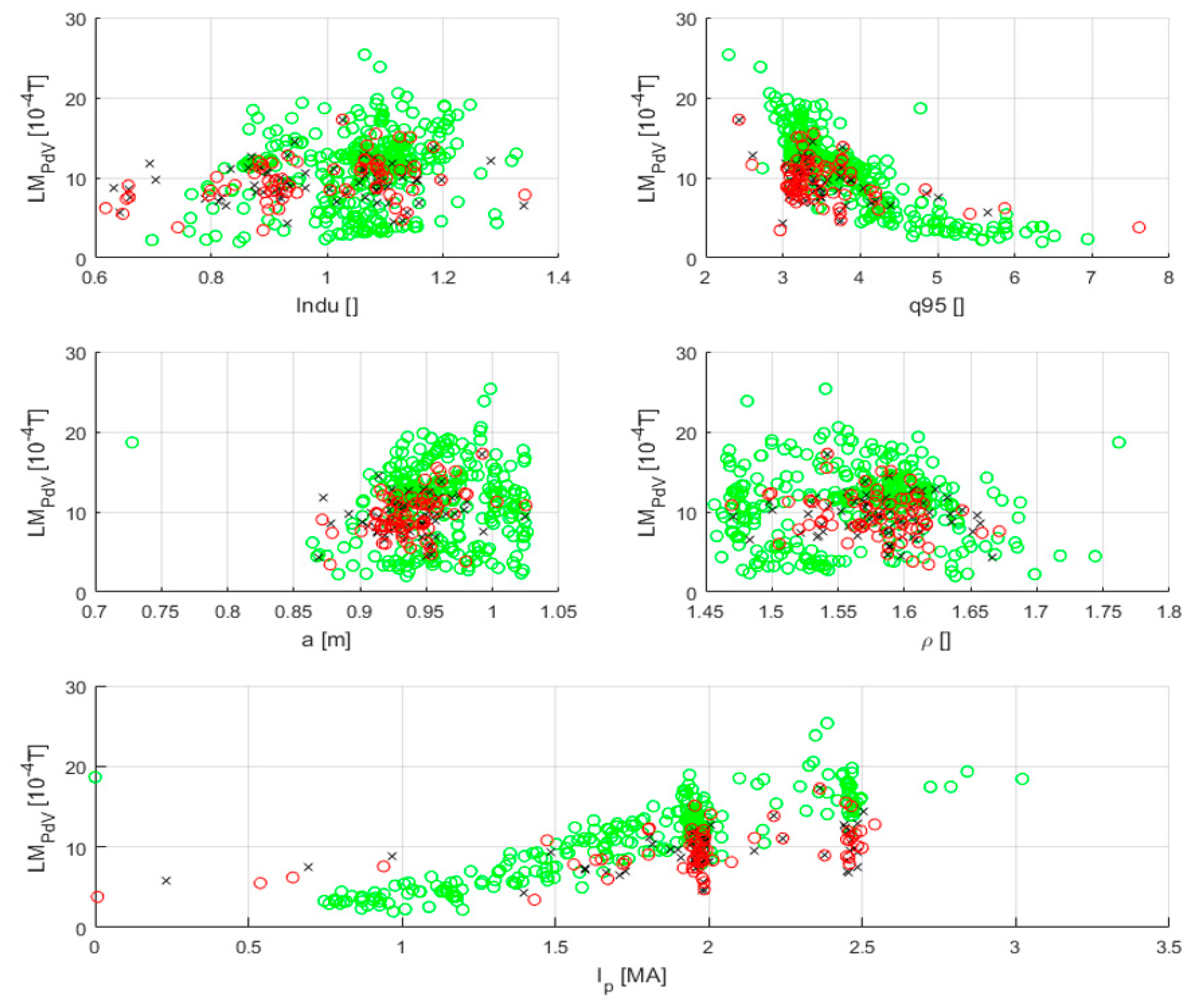
Unfortunately, Equation (3) does not fit the data of campaigns C29–C30 of JET with the ILW well. A first indication of the discrepancy between the equation and the data can be obtained by an inspection of the plots reported in Figure 7. For the 170 disruptions considered in the present study, the plots of Figure 7 report the critical value of the locked mode, as predicted by Equation (3), versus all the regressors. The values of the critical locked mode has been calculated with model (3) with the values of the parameters suggested in [45] at the following times: at the time slice of the alarm (when the experimental locked mode reaches the critical value predicted by the equation) and 15 ms before the beginning of the current quench. The estimates of the critical threshold have also been calculated for the flat top phase of the same discharges. From the plots reported, it can be easily seen that, before the beginning of the current quench, there is full overlap between the estimates for the flat top and the pre-disruptive time slices. Therefore, these estimates are not useful for prediction. This has been verified by testing the performance of the critical value of the locked mode proposed in [44] for the entire C29–C30 campaigns (for a total of 170 disruptive shots and 987 safe discharges). Again, all the time slices with plasma current higher than 750 kA have been included in the analysis. The final statistics are reported in

Table 3. The traditional figures of merit to assess the performance of predictors for the case of Equation (3) applied to campaigns C29–C30.

Method	Success Rate	Missed	Early	Tardy	False	Mean (ms)	Std (ms)
Equation (3)	52.35% (89/170)	24.12% (41/170)	0% (0/170)	23.53% (40/170)	1.72% (17/987)	175	328

and

Table 4. Performance of Equation (4) for Campaigns C29–C30.

Method	Success Rate	Missed	Early	Tardy	False	Mean (ms)	Std (ms)
Equation (4)	91.7% (156/170)	1.2% (2/170)	0% (0/170)	7.1% (12/170)	2.3% (23/987)	338	357

, from which it can be appreciated how the success rate is certainly less than satisfactory.

Even if Equation (3) does not seem to provide very useful information for prediction in JET with the ILW, at least for the campaigns analysed, the set of quantities proposed contains signals, which are unquestionably very important. In particular the locked mode and the internal inductance have proved to be essential also in the analysis reported in Section 5. Therefore, it can be argued that it is the power law form of Equation (3), which is not adequate to model JET data. The probabilistic SVM and the CART ensembles have therefore been applied to the regressors used in Equation (3) to derive the critical value of the locked mode signal. The models derived present very good performance; the success rate is about 95% and the false alarms are 5% again for a comfortable range of threshold probabilities. Therefore, the ML models perform slightly worse than the one of Equation (1) but are very competitive.

The main reason for the better performance of the machine learning models, compared to Equation (3), resides as expected in the functional form of the final equations: the machine learning tools are not limited to power laws. Unfortunately, the technique proposed in this paper, to convert ML models into realistic equations, is not viable for such a high number of regressors. Indeed, the dimensionality of Equation (3) is too high and the number of disruptions insufficient (by orders of magnitude). In such a number of dimensions, the points are too sparse in the hyperspace and it is not possible to reconstruct robustly and reliably the boundary. This is not a limitation of the methodology but a consequence of the excessive sparsity of the available data (the so-called curse of dimensionality). On the other hand, the number of really relevant quantities for JET is three: locked mode, internal inductance and q95. The others, such as the distance between the plasma boundary and the location of the coils measuring the locked mode, are introduced in [44] for the purpose of deriving a multimachine scaling, which is not the objective of the present study. In three dimensions, it is still possible to apply the proposed methodology of SR via GP with 170 disruptions as examples. Deploying again the probabilistic SVM and the CART ensembles, it has been found that the models provide a good compromise between success rate and false alarms. 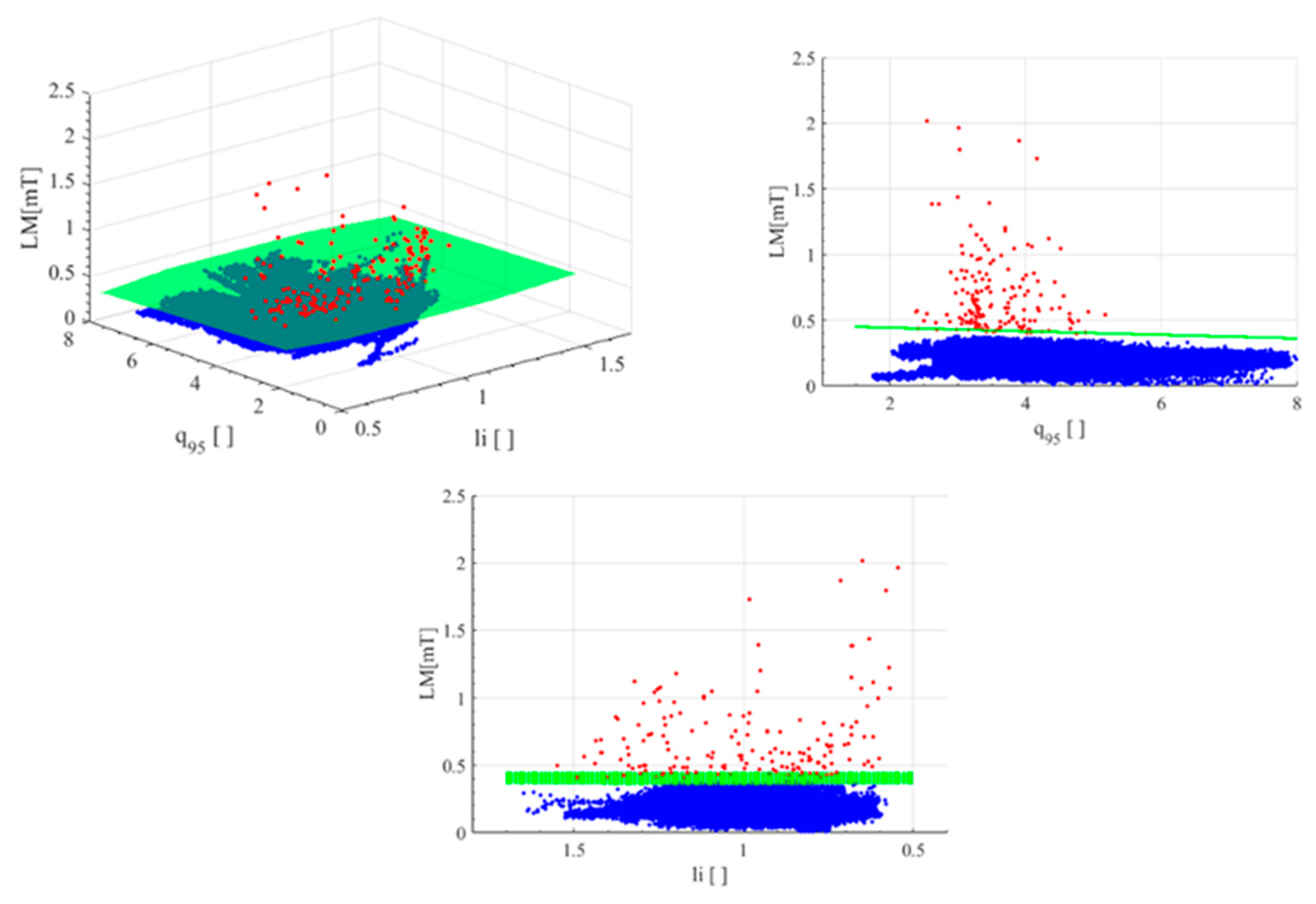The methodology described in Section 3 has then been deployed to obtain the equation of the boundary between the safe and disruptive regions of the operational space. The original range of the variables (including disruptive and non-disruptive samples) is: LM ϵ [0.0030, 3.1] mT, q95 ϵ [2.07, 7.81], li ϵ [0.45, 1.64]. The function to be identified expresses the critical locked mode amplitude as a function of the internal inductance and q95, i.e., f(x,y) = LM(li, q95). The obtained equation reads:

$$LM=0.475-0.017·{q_{95}}^{0.95}-0.014·l{i}^{1.00}$$

(4)

with the amplitude of the locked mode signal LM in mT. Here again, only one model is reported for the same reasons adduced in the previous section when discussing relation (1).

The plots of Figure 8 show how Equation (4) fits the boundary between the safe and disruptive regions of the operational space. The good quality of the obtained model can be appreciated by inspection of Table 4 for the campaigns C29 and C30 used for the training.

Again, to prove the generalisation potential of the derived boundary equation, relation (4) has been applied to the discharges of campaign C31, which are completely new examples never seen by the predictors. The good discrimination capability of the model, shown in

Table 5. Performance of Equation (4) for campaign C31. The models obtained at the end of C30 have been applied to the examples of C31 without any retraining.

Method	Success Rate	Missed	Early	Tardy	False	Mean (ms)	Std (ms)
Equation (4)	92.21% (142/154)	3.25% (5/154)	0.65% (1/154)	3.9% (6/154)	11.93% (52/436)	424	484

, confirms once more that the methodology proposed manages to converge on an interpretable but preforming equation. The degradation of performance in terms of false alarms is a problem of obsolescence, due to the rapidly varying experimental conditions in C31 and indeed affects in the same way also the ML models.

It is worth mentioning that it has been verified that practically the same results can be obtained using the traditional SVM instead of the probabilistic version. Therefore, the results of the investigation with the proposed combination of machine learning tools indicate that the quantities considered in the model of Equation (3) are very informative about disruptions. On the other hand, the equation of the boundary has a different form and in particular it cannot be represented by a simple power law. This conclusion is in quite good agreement with the results presented in [44], where it is shown that power laws do not fit well JET data. Indeed, the goodness of fit for JET reported in [44] is quite low in the variable space discussed in this section.

With regard to the interpretation of these results, the basic physical explanation proposed in [44] seems to be confirmed (even if the power law formulation of the model is probably not adequate). In practical terms, Equation (4) indicates that the configuration stability becomes more delicate as the internal inductance and the q95 increase, since at higher values of these quantities the plasma can tolerate a smaller value of the measured locked mode amplitude before disrupting. The increase in these parameters corresponds to a shift inward of the rational surfaces, on which the magnetic islands are typically centred. The same amplitude of the locked mode, as detected by the external saddle coils, therefore corresponds to larger islands when li and the q95 are higher. Plasmas affected by larger islands are reasonably more prone to disrupting.

One of the most relevant aspects of Equation (4) is the almost linear dependence of the locked mode on the internal inductance and q95 (instead of a power law type of scaling). In the next JET campaigns, this is an important aspect to be confirmed, possibly with dedicated experiments. On the other hand, the fact that the dependence becomes exponential, when reducing the feature space to two dimensions, as shown in Section 5, is a typical mathematical consequence of the contraction in the parameters. The fact that boundaries tend to become hyperplanes in higher dimensions is indeed the principle on which SVMs are based [30]. However, the change in the mathematical form, depending on the dimensionality of the parameter space, emphasises the importance of exploratory techniques, such as SR via GP, which do not assume a priori the model expression but can derive it directly from the data.

7. Conclusions and Future Prospects

In this paper, it is shown how it is possible to derive reliably an equation for the boundary between safe and disruptive regions of the operational space directly from the classification provided by machine learning tools. The methodology has been exemplified with two of the most popular types of classifiers, namely SVM and ensembles of CART. The goal is achieved by an original application of Symbolic Regression via Genetic Programming, which proves the further applicability of these techniques compared to previous investigations [29]. Practically the same model is found with either ML tool. The performance of the derived equations, in terms of success rate and false alarms, is practically the same as the original machine learning tools. It can therefore be concluded that the equations, derived by Symbolic Regression via Genetic Programming, match the ones of the machine learning tool models and therefore inherit all their qualities and drawbacks. As a consequence, the critical aspect to obtain valid equations is the quality of the statistical basis used to train the machine learning classifiers.

The data driven models, obtained with the methodology described in the paper, clearly outperform by a factor, if not by one order of magnitude, traditional empirical models based on representations such as the Hugill or the beta limit plots. The derived relations for the boundary are also orders of magnitude easier to interpret than the models of the original ML tools. Indeed, traditional SVM for the problem at hand typically comprise hundreds of Gaussian functions centred on an equal number of support vectors. The ensembles of CART classifiers typically require many hundreds of trees to obtain reasonable performances. Therefore, the developed techniques can be tuned to find the best trade-off between complexity and realism; the derived models are of a manageable complexity and, at the same time, do not oversimply the problem at the expenses of poor success rates like the power laws recently proposed. Moreover, by appropriate selection of the Symbolic Regression basis functions, it is possible to obtain equations with physical meaning, which can be compared with theory or used to guide model developments. It is worth emphasizing that the formulation of the equations in a more physically meaningful form does not cause any appreciable reduction in the success rate of classification. Therefore, these equations can be usefully deployed also in real-time networks for the prediction of disruptions. Moreover, a series of exhaustive tests has proved that the proposed methodology can be applied also to the models obtained with adaptive training from scratch of the type reported in [28,29].

It is important to notice that the analysis presented shows very clearly how, at least in the features space investigated in the paper, the boundary between the safe and disruptive regions of the operational space can have a quite different mathematical form, depending on the number of regressors used. In the case of two independent variables, the equation of the boundary is an exponential whereas in a three-dimensional space becomes a linear equation. This emphasises the importance of the methodology proposed, which does not force a priori the models to have any predefined mathematical form. Moreover, power laws have not proved to be very useful expressions for the boundary on the operational space in JET with the ILW, confirming the preliminary indications reported in [42]. Consequently, the present work confirms the limitations of power laws for the investigation of thermonuclear plasmas, as already reported extensively for the energy confinement time and the radiation limit [46].

With regard to the machine learning aspects of the approach, the methodology described in this work generalises the one pioneered in [26]. SR with GP can be applied nowadays to practically any type of classifier. To those, which can output a probability, exactly the same procedure used for the probabilistic SVM and CART can be directly implemented. For the others, the necessary points on the boundary can be extracted with algorithms similar to the one described in the detail for the traditional SVM in Section 3.1.

In terms of future developments, one of the main priorities is certainly the applications of the developed methodology to support avoidance strategies [46,47], which will certainly require the refinement and use of new diagnostics particularly spectroscopy [45] and polarimetry [48].