Multi-Gene Genetic Programming Regression Model for Prediction of Transient Storage Model Parameters in Natural Rivers


1
Department of Civil and Environmental Engineering, Seoul National University, Seoul 08826, Korea
2
Korea Institute of Civil Engineering and Building Technology, 283, Goyangdae-ro, Ilsanseo-gu, Goyang-si 10223, Gyeonggi-do, Korea
*
Author to whom correspondence should be addressed.
Water 2021, 13(1), 76; https://doi.org/10.3390/w13010076
Submission received: 25 November 2020
/
Revised: 23 December 2020
/
Accepted: 25 December 2020
/
Published: 31 December 2020
(This article belongs to the Special Issue Contaminant Transport and Fate)
Abstract
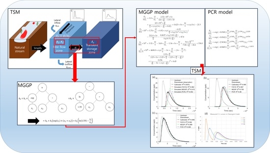
:A Transient Storage Model (TSM), which considers the storage exchange process that induces an abnormal mixing phenomenon, has been widely used to analyze solute transport in natural rivers. The primary step in applying TSM is a calibration of four key parameters: flow zone dispersion coefficient (), main flow zone area (), storage zone area (), and storage exchange rate (); by fitting the measured Breakthrough Curves (BTCs). In this study, to overcome the costly tracer tests necessary for parameter calibration, two dimensionless empirical models were derived to estimate TSM parameters, using multi-gene genetic programming (MGGP) and principal components regression (PCR). A total of 128 datasets with complete variables from 14 published papers were chosen from an extensive meta-analysis and were applied to derivations. The performance comparison revealed that the MGGP-based equations yielded superior prediction results. According to TSM analysis of field experiment data from Cheongmi Creek, South Korea, although all assessed empirical equations produced acceptable BTCs, the MGGP model was superior to the other models in parameter values. The predicted BTCs obtained by the empirical models in some highly complicated reaches were biased due to misprediction of . Sensitivity analyses of MGGP models showed that the sinuosity is the most influential factor in , while , , and , are more sensitive to . This study proves that the MGGP-based model can be used for economic TSM analysis, thus providing an alternative option to direct calibration and the inverse modeling initial parameters.
1. Introduction
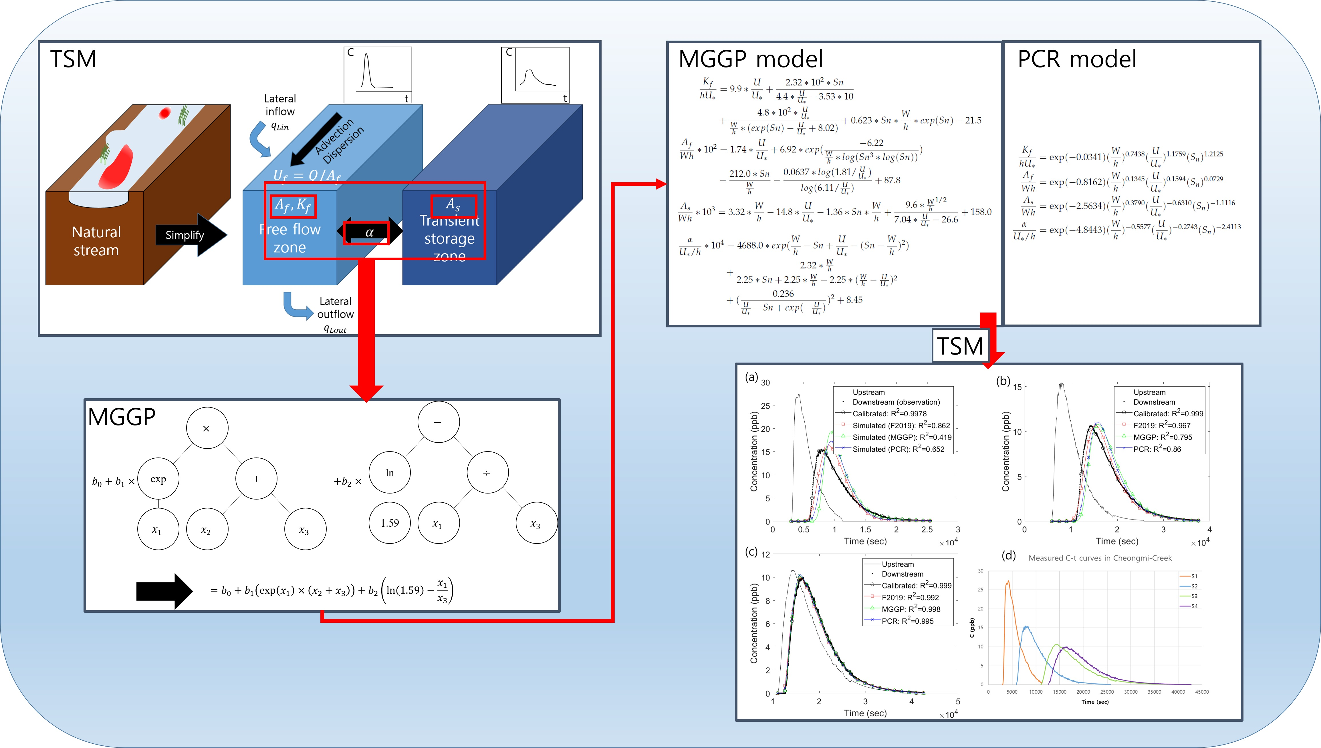
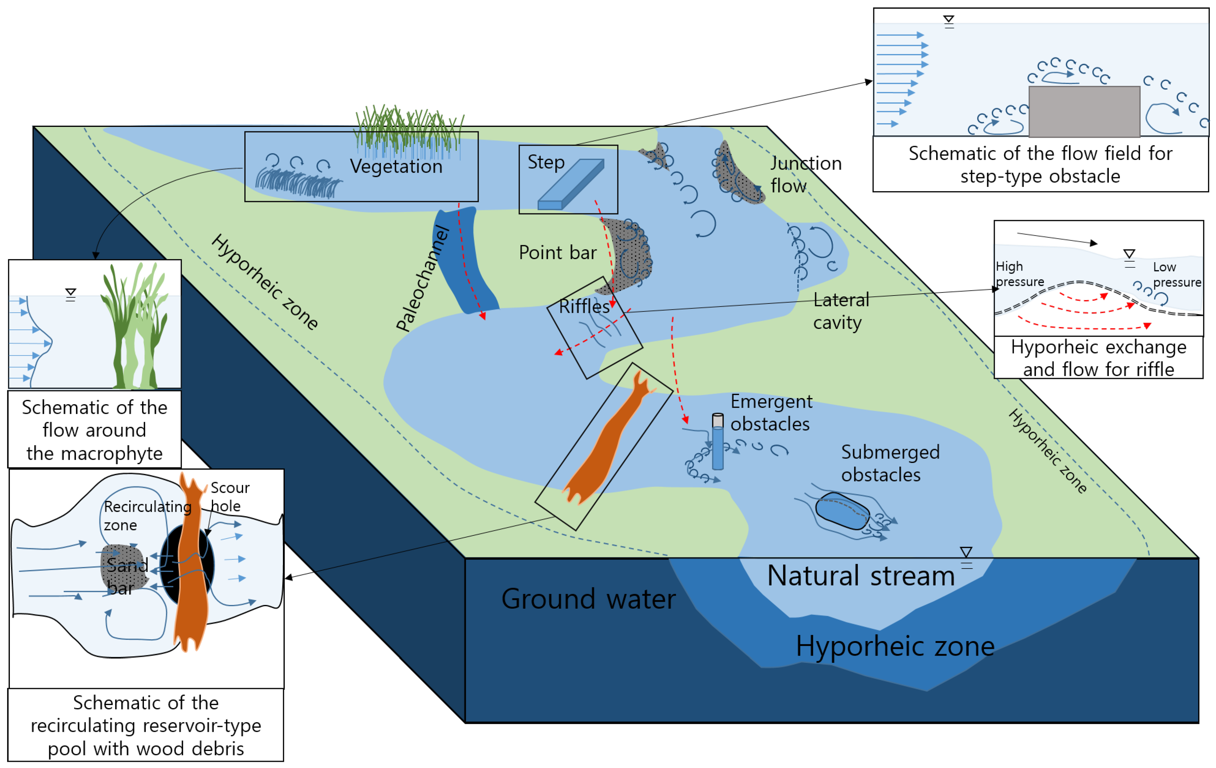
Precise prediction of solute transport in natural streams is essential to management of water quality in rivers. To analyze the fate and transport process of solutes, tracer testing using a conservative or non-conservative tracer is a one straight forward method used in many solute transport studies. In order to analyze solute transport mechanisms with a tracer test, assessment and measurement of hydraulic and, geomorphic properties and breakthrough curves (BTCs) are necessary. The obtained BTCs are used for straight analysis and estimation of solute mixing parameters in mixing analysis models. However, in a natural river system, analysis of the fate of solutes requires quantification of the effects of transient storage zones, including factors such as bed material, pool-riffle, channel meander, artificial hydraulic structures, and aquatic vegetation (Figure 1). In Figure 1, the red dashed lines indicate the hyporheic exchange, and solid navy lines indicate free flows through surface transient storages. These transient storage zones drastically influence flow structure and cause anomalous dispersion characteristics which cannot be simulated using a conventional one-dimensional advection dispersion equation model (1D-ADE) as shown in Figure 2. Thus, previous research has advocated models that account for the effect of transient storage rather than 1D-ADE in order to better represent skewed BTCs with long tails [1,2,3,4,5,6,7,8,9,10].
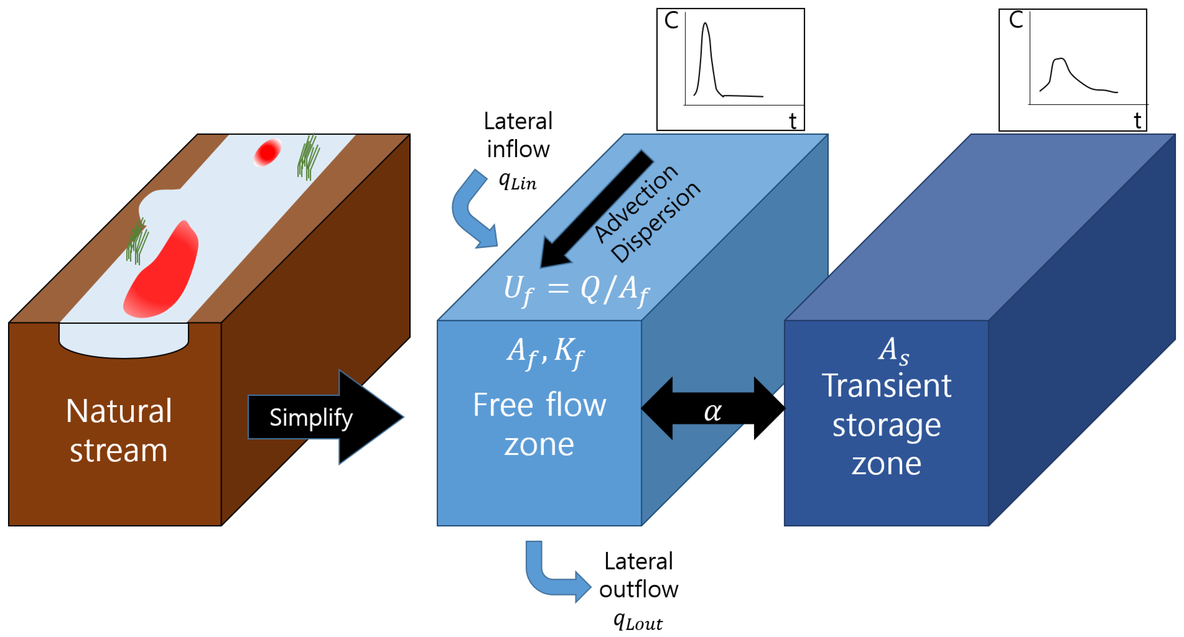
In order to solve the anomalous mixing problem shown in Figure 2, many efforts have focused on the development of phenomenological models that simulate the BTCs observed in natural tracer tests [17]. Representative models that were developed over the past decades include the following: conventional Transient Storage Model (TSM) [10], multiple zone TSM [18], Fractional advection-dispersion equation model (FADE) [19], Modified advection-dispersion model (MADE) [20], Multirate Mass Transfer Model (MRMT) [21], Advective Storage Path Model (ASP) [22], Continuous Time Random Walk approach (CTRW) [23], Solute Transport in Rivers (STIR) [24], and Aggregated Dead Zone (ADZ) [25]. Those models are continuously updated in order to reflect real mixing phenomena. Among the phenomenological models that consider transient storage, TSM is the most widely used solute transport model. TSM imitates the complicated natural river mixing process due to transient storage by simplifying the perpendicular mass exchanges between two zones, a mobile zone (main flow zone) and an immobile zone (storage zone) as shown in Figure 3.
TSM requires calibration of four key parameters, which are main flow zone dispersion coefficient (), main flow zone area (), storage zone area (), and mass exchange rate (), by inverse modeling in which best fit parameters can be found by matching simulated BTC to the measured curve. In particular, one-dimensional transport with inflow and storage (OTIS), which is a finite difference method numerical model, and its parameter estimator OTIS-P are common software tools used for TSM analysis [26]. However, many investigators have reported that the OTIS-P suffers from the equifinality problem that the calibrated TSM parameters may be local optima or unreasonable parameter sets [27,28]. Several investigators have attempted to overcome the local minima problem by adopting meta-heuristic optimization algorithms [16]. Even though the meta-heuristic optimization methods have an advantage over local search algorithms, there is a problem in that the estimated TSM parameter values differ given different curve similarity criteria [16]. From another point of view, many researchers have focused on identifying the properties that contribute to uncertainty in TSM parameter estimation [25,26,29,30]. For example, a study that took the TSM parameter combination point of view showed that the value of experimental Damkohler number (), which is the ratio of solute advection and the storage effect, in a reasonable range [0.5 10] has less uncertainty, so is used as a reference value in reasonable TSM parameter estimation [29]. In order to overcome uncertainty, uncertainty software tools were developed using statistical approaches, such as Monte-Carlo analysis [28], and a generalized likelihood uncertainty estimation (GLUE) framework [30]. On the other hand, a recent study spotlighted the computational points of TSM, and proved that computational conditions such as grid size () and computational time step () affect the result of TSM parameter estimation since numerical models have numerical errors [31]. Overall, TSM parameter estimation using inverse modeling has a primary limitation in that it requires BTC measurement data and hydraulic data from tracer tests for every parameter estimation. For this reason, conventional parameter estimation methods are infeasible for mixing studies of large-scale rivers. For example, recent studies exploiting the solute transport models pay attention to the contaminant source identification problem [32,33,34]. However, such studies are conducted under the assumption that the mixing parameters are known since both 1D-ADE and TSM require calibration of parameters using inverse modeling, which is a high-cost method with a great deal of uncertainty. More specifically, users have to re-estimate TSM parameters when discharge or bed-form change, even at the same stations since hydraulic properties, which influence TSM parameters, have changed.
To overcome the drawbacks of parameter estimation with inverse modeling, empirical equations to calculate the properties of transient storage have been developed by analyzing their relationship with hydraulic features, such as velocity, shear stress, and shape-related factors in cross-section [4,10,35,36,37,38,39,40,41]. Jackson et al. [15] comprehensively classified hydromorphic factors accounting for diverse surface transient storage (STS) factors that exert sudden changes in flow structure, apart from hyporheic transient storage (HTS). An additional accessible feature that explains STS in that article is a morphological feature, channel sinuosity (). Similarly, most of empirical equations used to estimate hte 1D-ADE dispersion coefficient are functions of cross-sectional width (W), mean hydraulic depth (h), mean velocity (U), and shear velocity () [42,43,44,45,46,47,48,49]. Early works that took a regression approach to TSM parameter estimation focused on relating hydraulic properties using only storage area ratio . Recent studies produced extra parameters accounting for transient storage zone, such as , the storage residence time , and [37,38,39,40]. Plus, a few studies [38,39] considered as an influential factor accounting for transient storage, but cannot be obtained unless BTCs are available. More recently, a set of empirical equations for OTIS-based TSM parameters, , , and , were proposed. Femeena et al. [40] carried out a meta-analysis of various published studies on river mixing tracer tests, and they included 1D-ADE dispersion coefficient, , values in the derivation of the empirical equation for the main flow zone dispersion coefficient, . It has been reported that has a larger value than for the same BTCs since TSM deforms BTCs by the composite effect of the four TSM parameters while 1D-ADE deforms BTCs with only [37]. The equations are based on non-linear regression analysis and finding equation forms by trial and error; equation forms uncovered by this approach can be restricted by the researcher’s intuition, so it is difficult to find hidden non-linear relationships. Even though previous equations are valuable since they do not require much information for estimation of the three TSM parameters, there have been no efforts to identify the main flow zone area, , using the empirical model since many investigators regard it is a deterministic value once hydraulic properties are measured in the tracer test. Thus, a complete model with the four key transient storage parameters (, , , and ) does not yet exist.
As data-driven approaches emerge, recently developed models have employed machine learning methods (e.g., support vector machine (SVM), artificial neural networks (ANNs), and symbolic regression techniques). Symbolic regression techniques have the advantage of producing explicit forms of equations, while the other machine learning methods produce implicit results. Taking an example of the water resource problem, multi-gene genetic programming (MGGP) was successfully utilized in daily streamflow prediction [50], and prediction of [41]. In accordance with the comparison study, genetic programming (GP) showed superior results compared to SVM and particle swarm model selection [51], whereas SVMs and ANNs have the potential for over-fitting and challenge of kernel parameter tuning results [52].
This study has three main objectives. The first aim of this study was to develop new dimensionless empirical equations for the complete set of TSM parameters, , , , and , that reflect the effects of both hydraulic and morphological features, using MGGP, which has been proven to be preferable in representing the non-linear behavior of the water quality variables as well as streamflow. In this study, we suggest new expressions for in the analysis since the main idea of TSM implies that can vary when other TSM parameters change, even though past efforts did not present an empirical equation for the main flow zone area . The second objective was to investigate the applicability of the proposed equations for a tracer injection experiment in a natural river, Cheongmi Creek, Korea. Consequently, one-at a time (OAT) sensitivity analysis was conducted for each empirical equation of the MGGP model in order to identify the major hydromorphic property of each TSM parameter. Thus, the objectives of this study were to present new alternative options for the TSM parameter estimation and to analyze the TSM parameters in terms of hydromorphic properties that are rather easily measured.
2. Models and Methods
2.1. Transient Storage Model
The fundamental idea of a TSM is to simplify complex natural river into a free flow zone and an immobile storage zone, as illustrated in Figure 3. After the first introduction of a TSM, the executable program OTIS was developed; it additionally considers lateral inflow and reactive solutes [26], and it is far the most popular TSM implementation [17]. TSM consists of a main flow zone equation (Equation (1)) and a storage zone equation (Equation (2)), where solutes are exchanged perpendicularly between the two zones.
where and are the concentration of the main flow zone and the storage zone, respectively []; Q is the discharge []; and are the area of the main flow zone and the storage zone, respectively []; is the dispersion coefficient in the main flow zone []; is the lateral water inflow []; is the concentration of the lateral inflow []; and is the mass exchange rate between the main flow zone and the storage zone [].
Remarks for the TSM
One-dimensional solute transport analysis is successfully applicable under the following three conditions: (1) statistically steady flow field; (2) constant cross-sectional area; (3) complete mixing over the cross-section [8]. However, even if the cross-sectional mixing is completed, the 1D-ADE simulation cannot be correct in complicated geometry, where skewed BTCs with a long tail are observed [45,53]. Nevertheless, if the characteristic length scale for variation is much larger than the channel variation, the longitudinal dispersion process in Equation (1) can be reasonable [53]. Complicated geometry accompanies storage zones where the solute is trapped. The streamflow area can be divided into the main flow zone and storage zone, and concentration difference induces the mass exchange mechanism between the two differed areas [54]. The TSM expresses the linear exchange process regarding the mass exchange coefficient and the storage area ratio, adopting the gradient induced mass exchange assumption (Equation (2)).
Since the TSM regards the cross-sectional area as a summation of the main flow zone and storage zone areas, it compels the assumption of instantaneous and uniform distribution of solute also in the storage zone. However, it is not easy to explain the simultaneous occurring of complex solute transport mechanisms (i.e., uniform distribution in the two cross-sectional areas, mass exchange, and no flow between adjacent storage areas) using this linear kinetic [10]. Despite, that a solute pulse is transiently trapped and release in storages in mountain streams. Accordingly, Equation (2), which models distributed transient storage zones along a flow path, is plausible [10].
As the coupled part of Equations (1) and (2) is replaced with residence time distribution (RTD), which determines how the tail of BTC decays, the TSM can be seen as the exponential distribution RTD model [22]. The exponential RTD is appropriate only under the well-mixed condition in both the main flow and storage zones [55]. Hence, the exponential RTD model underestimates the hyporheic exchange effect [56]. Experimental studies have proved that the power-law RTD fits better than the exponential RTD model, such as the TSM, as HTS contributes more [17,21,56,57,58,59,60,61].
2.2. Multi-Gene Genetic Programming
As previously mentioned, to analyze pollutant mixing in rivers using TSM, the parameters of the Equations (1) and (2) need to be estimated by either inverse modeling or empirical equations. In this study, new empirical equations for the set of TSM parameters were proposed using a multi-gene genetic programming (MGGP) model.
Genetic programming (GP) is a specialized genetic algorithm (GA) which is an evolutionary technique that mimics natural evolutionary processes such as mutation and crossover. The main difference between GA and GP is that GP evolves tree-based data structures while the GA evolves numeric vectors.
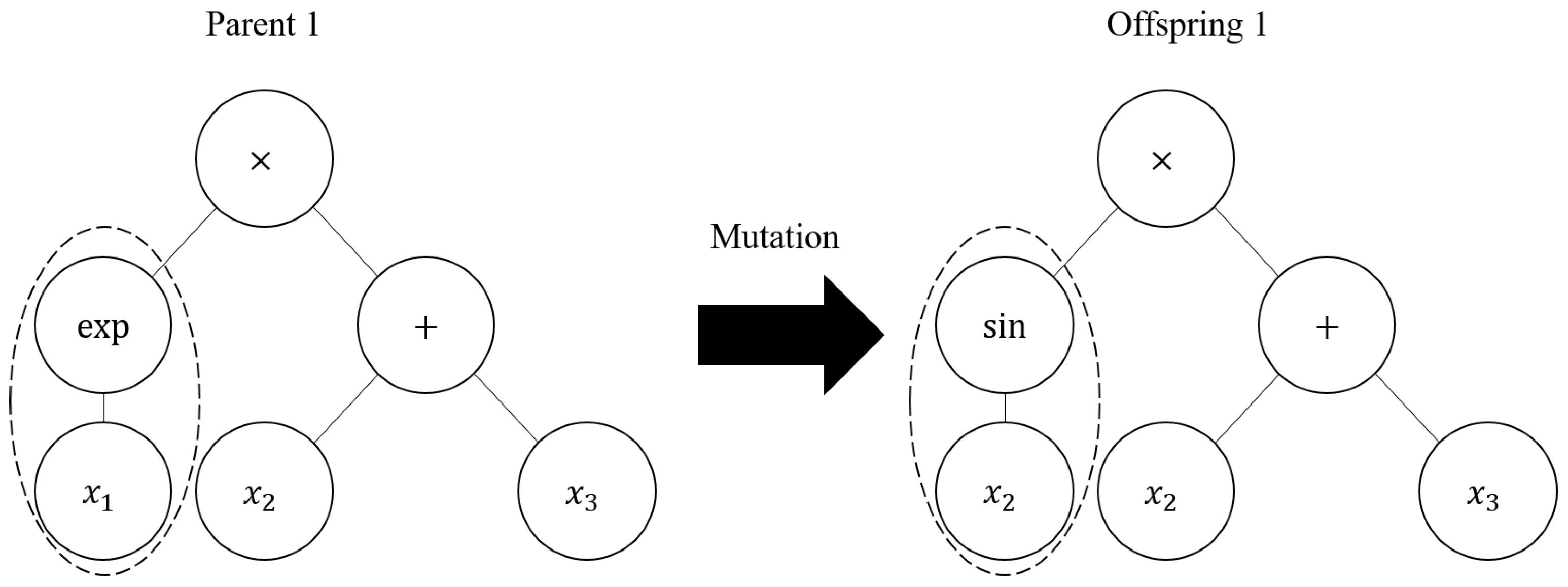
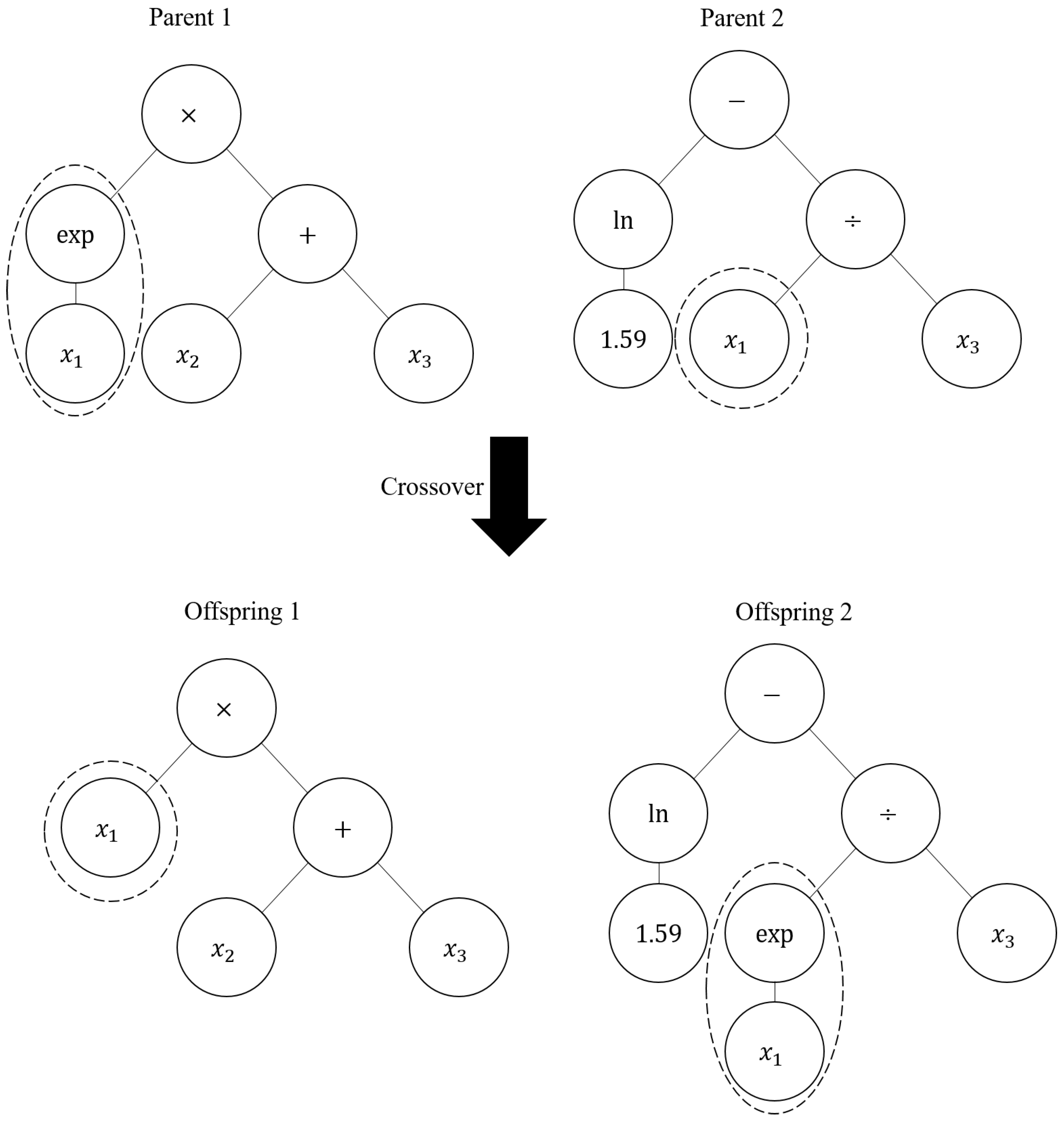
GP attempts to find the model with the optimal fit by constructing and modifying trees consisting of functions and variables. First, a random population of an individual gene is generated. Once the population of genes is randomly generated and fitness function values are evaluated, each gene is modified based on the principles of natural evolution with mutations and crossovers, thus producing offspring. The mutation process picks branches, along with sub-nodes, and replaces each bunch with a randomly generated subtree as depicted in Figure 4. For the crossover operation, terminals or branched nodes of parent trees are randomly selected, and the selected points are exchanged as depicted in Figure 5. Those two operations are applied to models with low fitness after the fitness value of each function is evaluated. This evolution step is iterated until the termination criterion is met, enhancing the fitness of the models produced from GP.
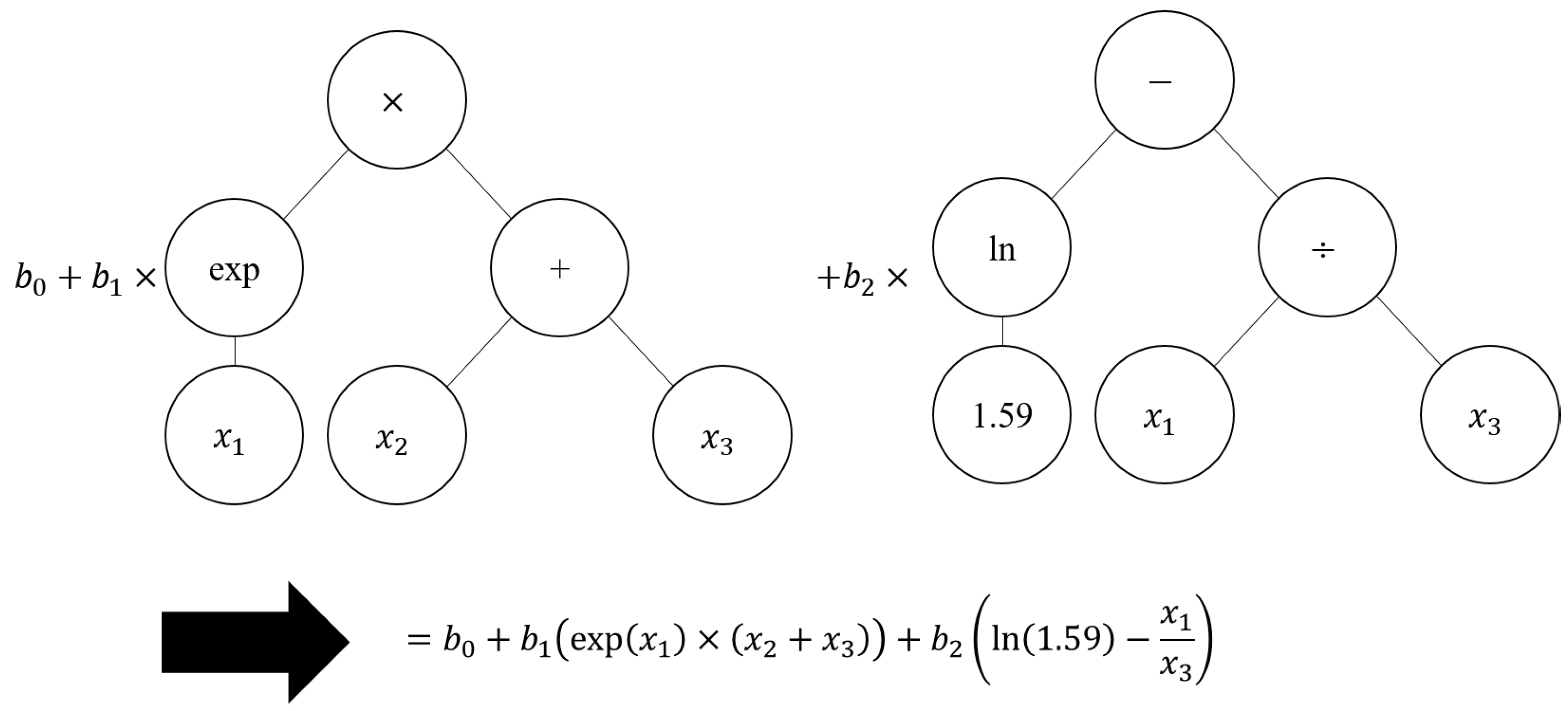
MGGP is a scaled symbolic regression method that is an advanced version of standard GP. The MGGP model is a linear weighted combination model consisting of individual gene-trees. The MGGP uses one or more gene-trees and calibrates coefficients of the gene-trees using statistical regression methods such as least-square regression. A typical example of MGGP model is shown in Figure 6, in which are the coefficients of the gene-trees.
As in standard GP, which iteratively reproduces new models using crossover and mutation procedures, the MGGP algorithm contains crossovers and mutations as well. The evolutionary processes in MGGP are so-called high-level crossovers and mutations, whereas those of standard GP are called low-level processes.
As a result of the operations done in MGGP, MGGP produces a bunch of equations, which are linear combinations of non-linear terms, without any pre-specified functional structure. In addition, the frequencies of variables in the obtained formulae reflect the relative importance of the variables. Subsequently, the MGGP approach offers more opportunity to catch nonlinearity associated with the phenomenon than does finding formula structures using the trial-and-error method.
3. Formulation of Empirical Equations
3.1. Dimensional Analysis and Data Collection
In order to develop generalized equations, dimensional analysis was performed based on Buckingham’s Pi theorem. As previously mentioned, past studies asserted that the hydromorphic properties contributing to the transient storage effect are morphological factors (such as channel meandering and cross-sectional shape), hydraulic conditions, and bed shear stress [13,15]. For example, Tonia and Buffington [13] explained that morphological parameters (e.g., channel meandering, pools, and riffle sequences) mainly drive the HTS exchange process. In addition, we summarized the relevant factors, which were easily obtained and the generally applcable properties, considering the classification of Jackson et al. [15], for STS, as in the following equation.
where, is the kinematic viscosity []; g is gravitational acceleration []; is the density of water []; W is the channel width [L]; h is the mean depth [L]; U is the mean velocity []; is the shear velocity []; is the mean bed slope [-]; is the channel sinuosity. According to [38,39], Froude number and Reynolds number did not show discerning relationships with the TSM parameters. Femeena et al. [40] excluded bed slope due to measurement uncertainty. Nevertheless, slope-based shear velocity and sinuosity were included as input variables in order to take all available features into account. Consequently, the functional relationships between dimensionless variables can be summarized as
Basically, a meta-analysis was performed in order to assemble sufficiently large TSM parameter values. OTIS-based TSM parameters were taken into consideration in the derivation of empirical equations. In particular, complete data sets, with the four TSM parameters (, , , and ) and hydromorphic properties (cross section, channel sinuosity, bed slope, and so on), were taken into account in the analysis. In the assembled data set, shear velcotiy, , was calculated using bed slope (Equation (5)).
Among 700 collections of meta-data, 128 datasets from 14 published papers [38,62,63,64,65,66,67,68,69,70,71,72,73,74] were adopted for this study by selecting data which provided all variables of the Equation (4) and satisfied . The meta-data list is available in the supplementary material. Noh et al. [16] assessed the applicability of optimization techniques for parameter estimation of the four TSM parameters. Using their parameter estimation setting, we exploited the meta-heuristic optimization method SC-SAHEL (Shuffled Complex-Self Adaptive Hybrid EvoLution) with a mean squared error (MSE), meta-data includes unpublished parameter estimation values from a tracer test conducted in Gam-Creek, Korea (Appendix A). A detailed description of the SC-SAHEL optimization algorithm is found in [75].
Even though the TSM parameters estimated by Cheong et al. [38] were based on the analytical solution of Hart [55], not OTIS, the estimated parameter values were included in the derivation under the assumption that the estimated parameter values would produce the same BTCs. Different expressions of the TSM parameters can be transformed using the following equations where is the storage zone ratio [-]; and T is the residence time [T].
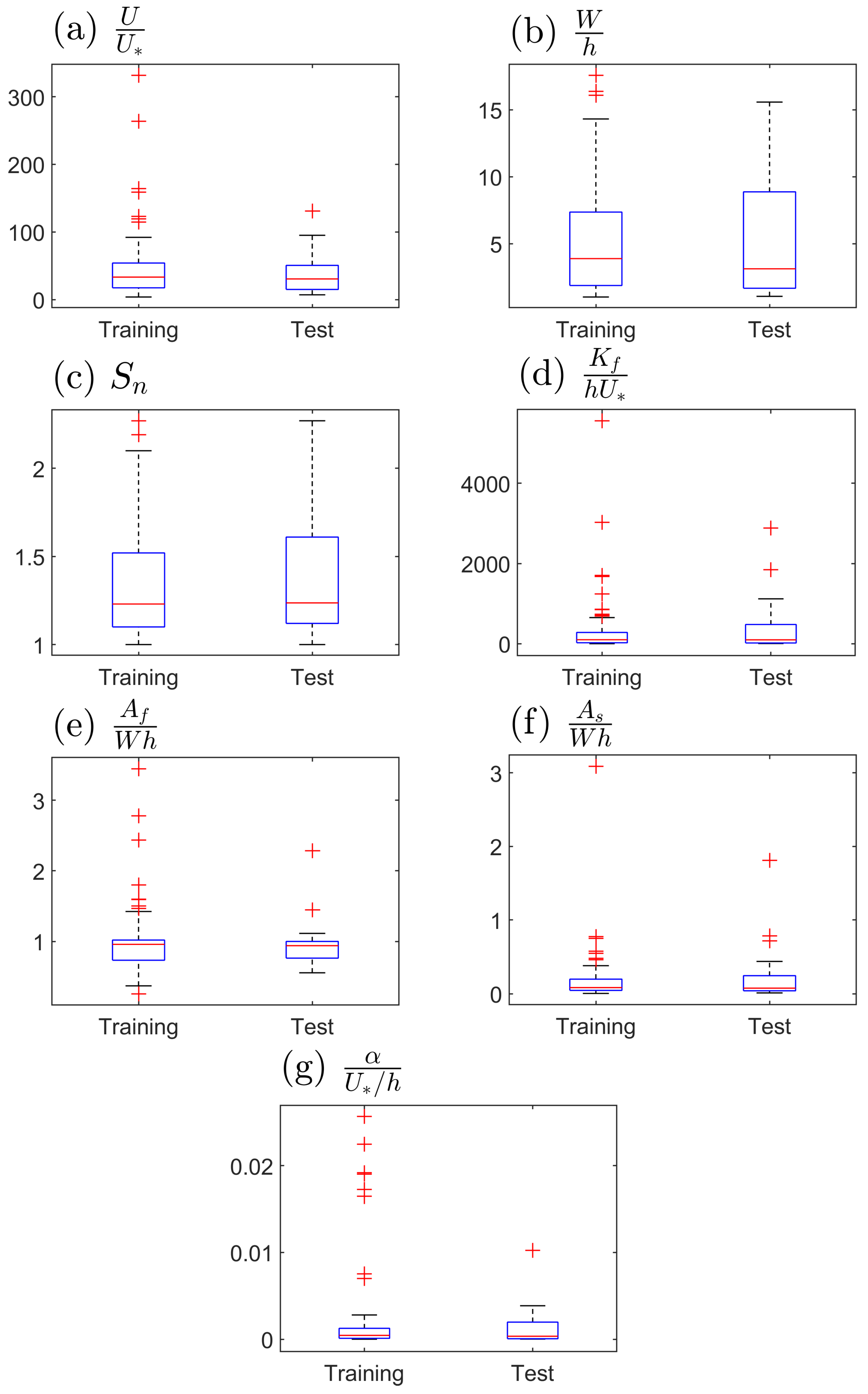
The chosen TSM parameter data were randomly divided into a training set (90), and a test set (38) in order to derive new equations. Table 1 presents simple statistics (minimum, maximum, and mean) for the dimensionless variables of the training set and the test set. In addition to the table, the simple statistics are shown as the boxplots in Figure 7. As shown in this figure, the total data range of the training set embraces the data range of the test set.
In order to consider the multicollinearity between dimensionless hydromorphic variables, variance inflation factor (VIF) values were calculated. The VIF is one of the criteria necessary for the evaluation of linear dependency between input variables in the regression analysis. It can be calculated with the following equation.
where is the calculated coefficient of variance for regression of the ith input variable on the other input variables. Generally, if VIF is greater than 10, then multicollinearity is said to be high. The calculated VIF values for the input variables , , and are 1.002, 1.005, and 1.005, respectively. Thus, there is no significant multicollinearity problem in the regression.
3.2. Formulated Equations
3.2.1. Formulation by MGGP
New MGGP expressions for the TSM parameters were derived using GPTIPS, which is the MATLAB library for MGGP [76]. MGGP evolves function terminals of the equations by following a specified function set. The four basic operators and power-based operators (power, square, cube, exp, and tanh) were nominated in the function terminal of MGGP. On the other hand, GPTIPS presents Pareto front models under two objective functions (model complexity and fitness) since over-fitting is a concern with high complexity models. In the same manner, MGGP was performed 200 times in a sequence of 500 generations for a population size of 500 for genetic operations in order to produce various forms of the Pareto front results. The maximum number of genes and the tree depth are directly related to the complexity of the produced equations since MGGP evolves in every iteration. Thus, in this study, the maximum depth and maximum number of genes were set to 6 and 4, respectively. The other hyperparameters, elitism, crossover relative parameters, and mutation parameters indicate the probability of a genetic operator’s activation in each generation, and those parameter values were chosen based on the previous study [41]. Table 2 summarizes the hyperparameter setting for MGGP in the present study.
The Pareto equations for each TSM parameter are given as follows.
3.2.2. Formulation by PCR-Based Regression
In order to test the empirical equations of the MGGP model, PCR-based regression equations were additionally derived using MATLAB’s LIBrary for Robust Analysis (LIBRA) [77]. PCR is a classical option for multiple linear regression, as it is robust even with correlated data and it makes it easy to interpret the input variables. The standard regression model defines an equation in the form , where is the observation maxrix; is the regressor matrix; is the regression coefficient matrix; and is the regression error. The main distinction of PCR is that it determines model coefficients from which is the eigenvector of . Using the orthogonality of , the general regression model of PCR can be expressed as
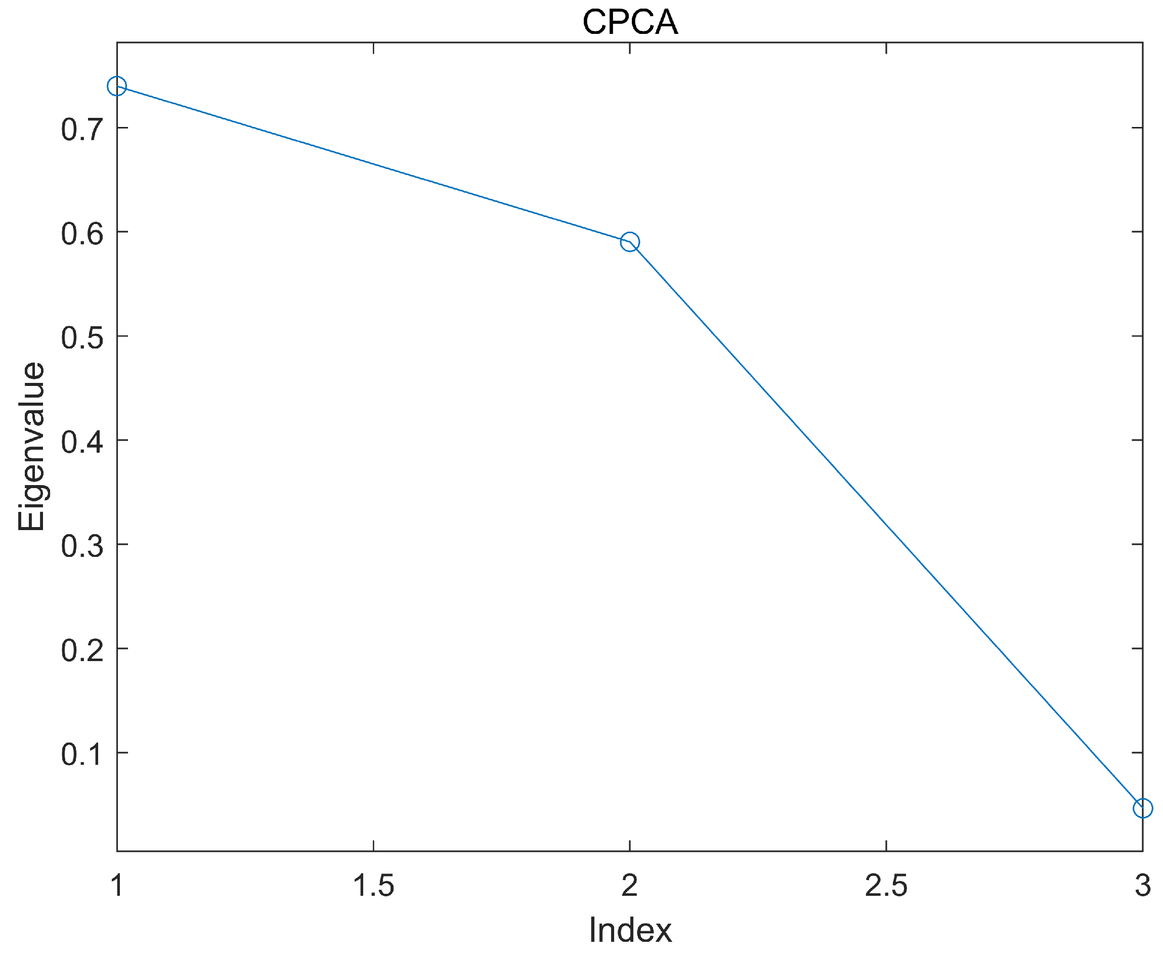
A scree plot was used to determine the number of principal components as shown in Figure 8. The recommended number of principal components is three since the cumulative eigenvalue is lower than 10% only with three principal components.
The empirical models using PCR were derived as:
The equations derived with both MGGP and PCR are in dimensionless form, but the MGGP equations had more complicated structures than did the PCR equations. The major difference between the two models was that the MGGP model considers the linear contribution of each input variable in addition to the nonlinear correlations. For example, had linear effects on Equations (11) and (12), and it could be expressed as independent terms. had two linear terms of and , but showed the most complicated formulation. Contrary to the MGGP model, we assumed that the structures of the four PCR equations are identical as per a pre-determined nonlinear power-law relationship. In addition, PCR equations using the total dataset were derived for expanded use but were not analyzed (see Appendix B). All derived equations are provided as MATLAB function files in the supplementary material.
3.3. Statistical Performance of the Models
In order to assess the performance of the proposed equations relative to published equations for the TSM parameters, simple regression Equations (20)–(22) presented in [40] were also considered in this study.
The equation set (Equations (20)–(22)) was noted as F2019 for brevity. Four performance criteria, accuracy, discrepancy ratio (DR), root mean squared error, coefficient of determination () and Pearson’s correlation coefficient () were evaluated to compare the performance of the equations.
where, and are the ith components of observed and the predicted target TSM parameters, respectively; and is the mean value of the observed TSM parameter.
Each calculated performance criterion is shown in Table 3. The bold characters in Table 3 indicate the best model for each performance criterion. The MGGP model predicted and with the highest accuracy. Compared to the PCR and F2019 equations, MGGP predicted with a reasonable degree of accuracy, even though the PCR model gave a slightly better result. The prediction of by MGGP showed low accuracy in both the training set and the test set. The accuracy of the other two models are about the same as that of MGGP for the prediction of .
The RMSE and results showed that the predictability of the MGGP model was good in terms of , , and in the training set. The PCR equations were good at predicting , , and in the test set, and the F2019 model for showed the lowest RMSE value over the training set. Regarding the test set, F2019 (Equation (22)) had the lowest RMSE and the highest values, but the MGGP model was the best model on average. The model with the best mean RMSE and was the MGGP model, except for .
In regards to , most of the models were higher than 0.5, but low values were observed in every model for prediction of . In particular, values for the training set using the MGGP formulae were closest to 1 for the training data, whereas PCR showed slightly more significant correlation in the test set. Still, the best performance of average were given by the MGGP predictions for every TSM parameter.
Briefly, the equations derived by MGGP gave the best performance in the training set and averaging performance of the training and test sets. The PCR equations showed stable performance and intermediate results between those of MGGP and F2019. The equations for and equations in F2019 performed fairly despite their simple formulations.
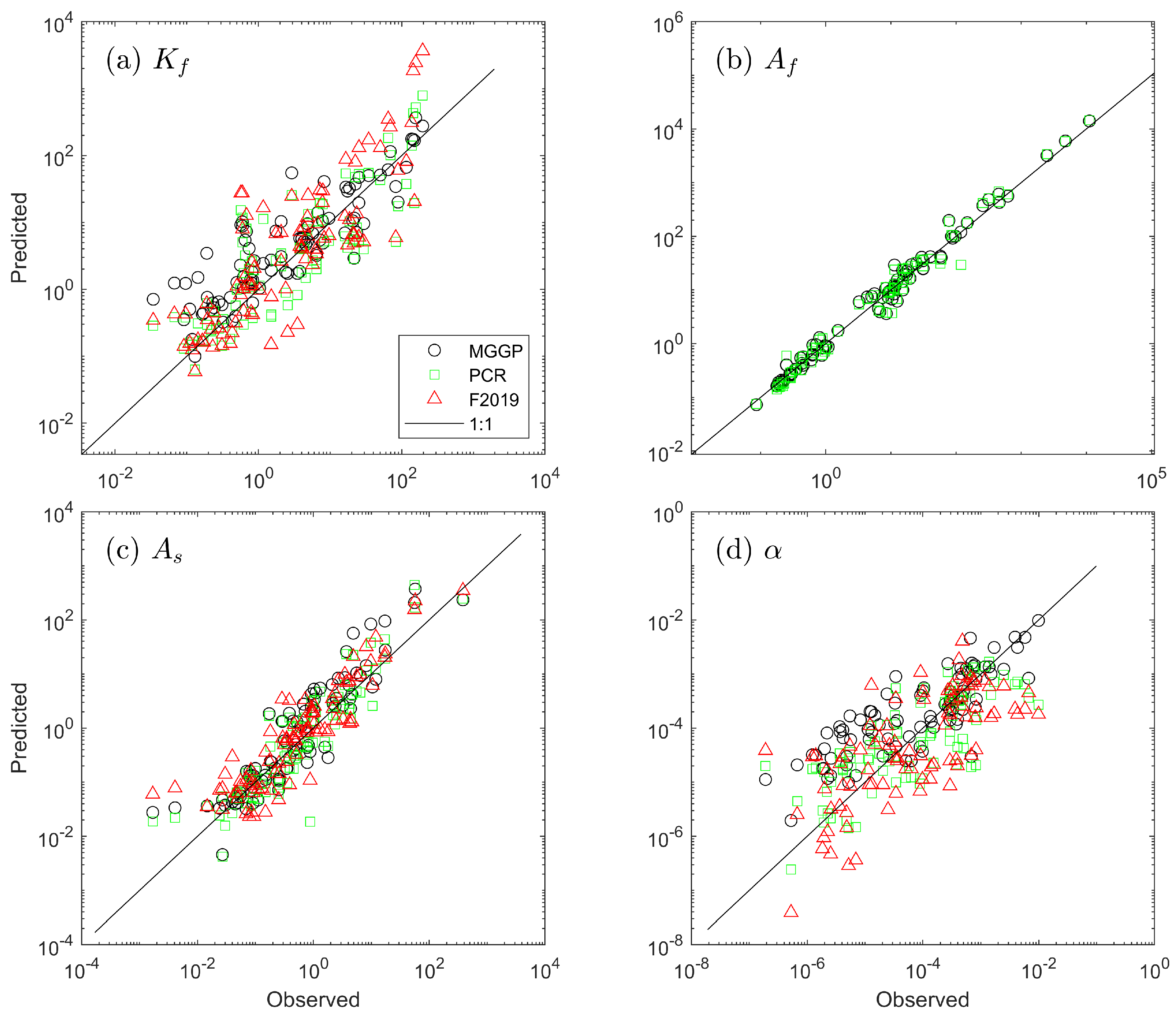
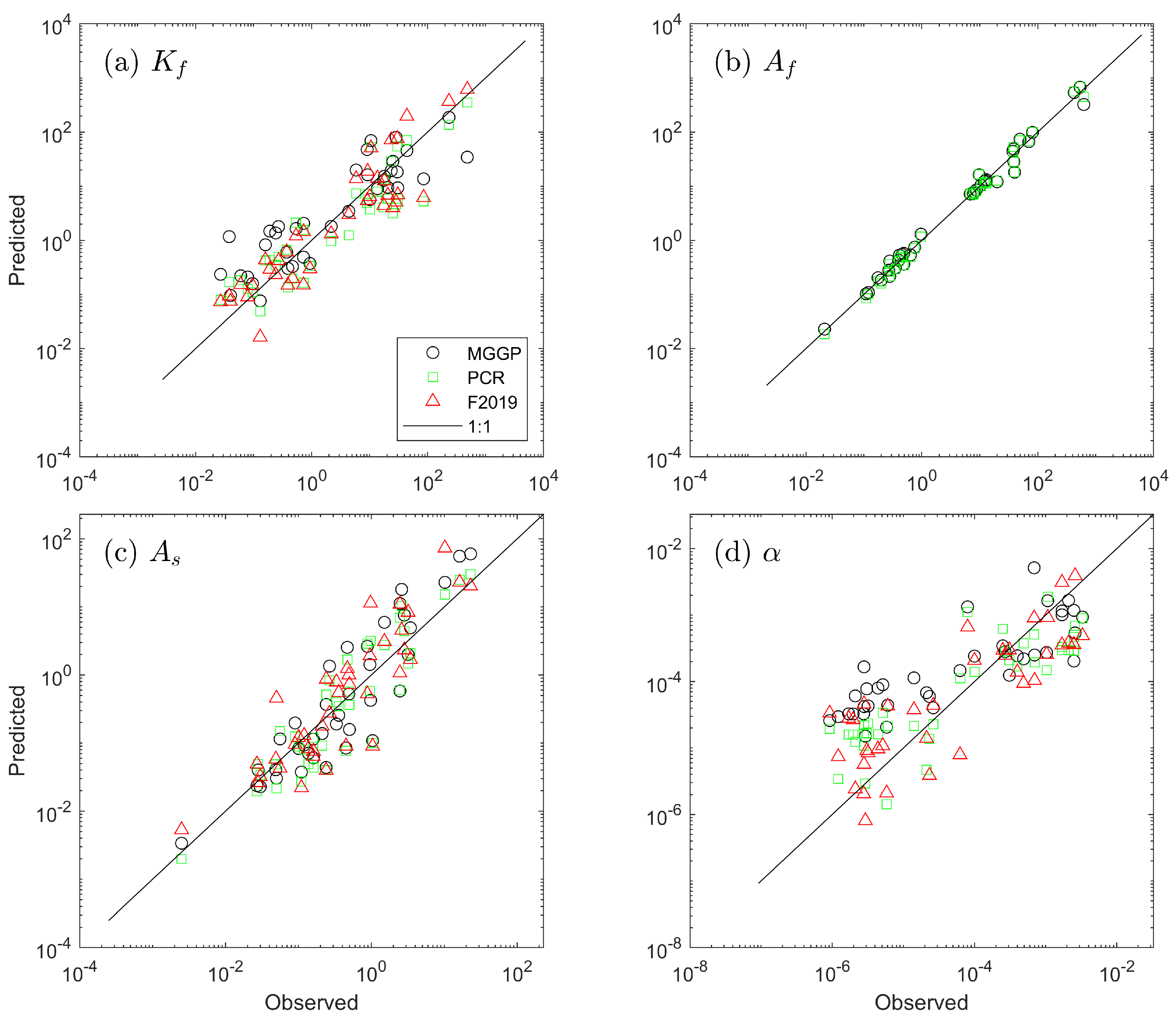
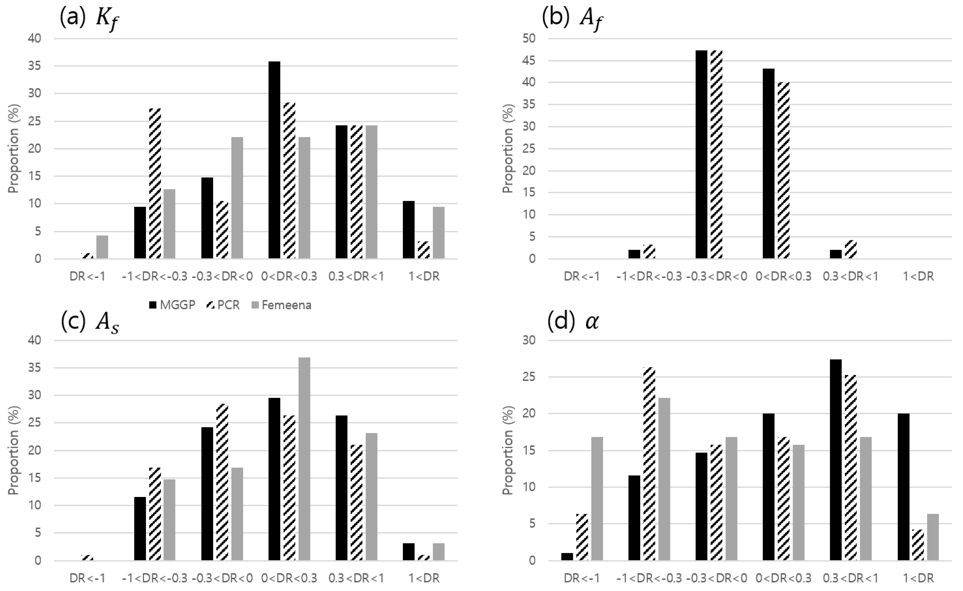
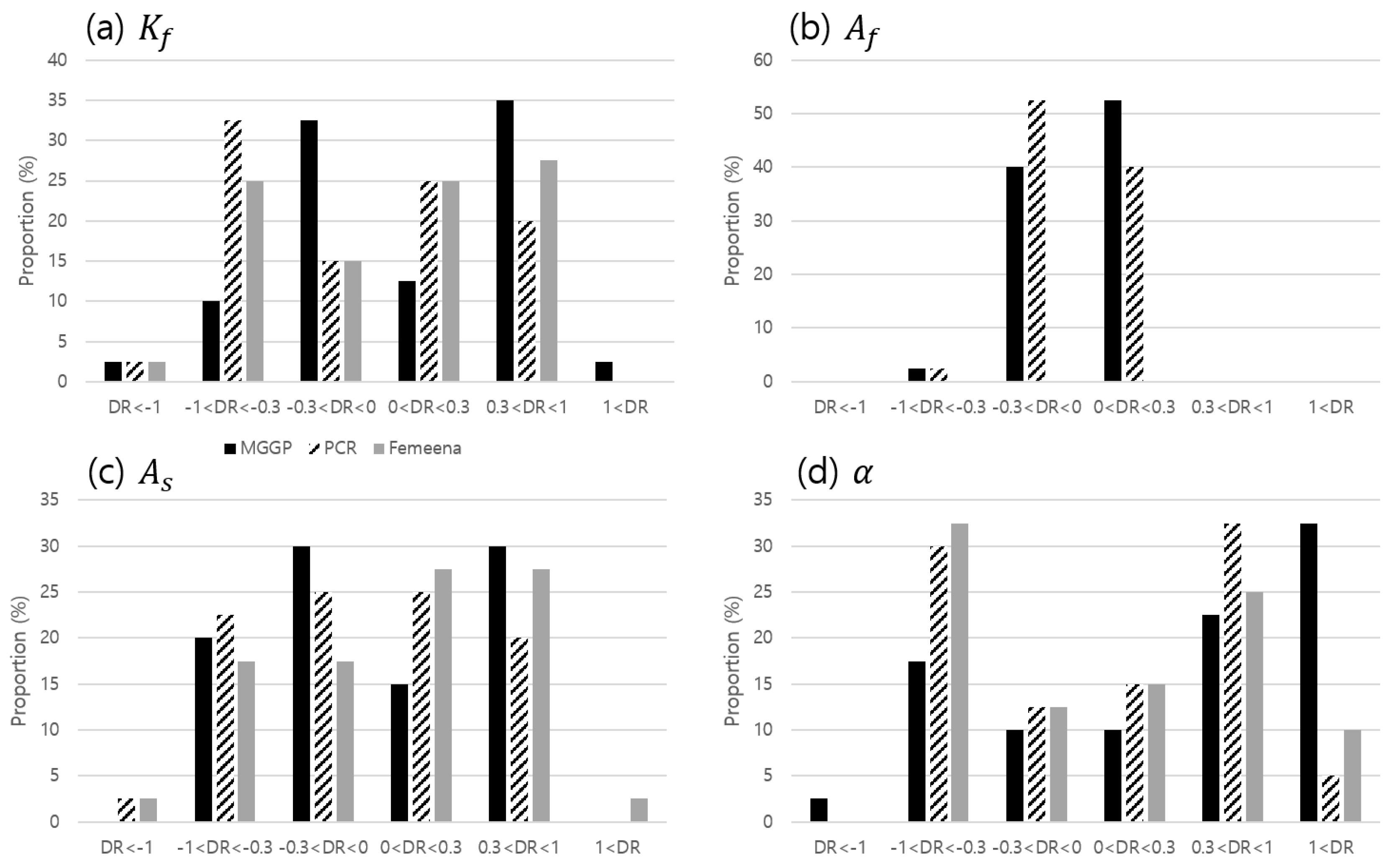
The prediction results are illustrated as acatter plots in Figure 9 and Figure 10. Furthermore, Figure 11 and Figure 12 present DR histograms, which represented the distributions of the predictions, of the training set and the test set, respectively. Figure 9a, Equation (20) overestimated , especially was large. As shown Figure 11 and Figure 12, high-variance distributions were obtained using Equations (16) and (20) in both the training and the test set. The MGGP model presented the smallest deviation in . Both the MGGP and the PCR models for presented similar results. In , three equations better predicted the training set than the test set in the range of . Figure 9 and Figure 10 showed that the predictions of by all equations are scattered. These discrepancies are clearly demonstrated the DR histograms depicted in Figure 11 and Figure 12. Every model had difficulty when used to predict the test set of , with double-peaked distributions. In particular, the MGGP model over-estimated . According to the presented figures, the PCR formulae, which were in the range of , gave the most stable overall performances.
From the results of the scatter plots and the DR histograms, the empirical equations predicted the two-dimensional shape variables ( and ) more accurately than the solute mixing related variables ( and ). It implies that the three hydromorphic variables, , , and , are not enough to describe the complicated physical mixing process in natural rivers where a number of transient storages are arranged, as shown in Figure 1. Unfortunately, adopting more variables is not easy. Therefore, even recent empirical approaches to the 1D-ADE’s dispersion coefficient are adopting and due to the limitations of knowledge in physical process and measurement technique [41,48,49,78].
Large errors in predictions of and may be produced from the TSM model error. As aforementioned, the TSM considers only the bulk shear dispersion in the main flow zone, and it treats transverse mass exchange at the storage zone boundary. This weakly two-dimensional vision neglects the transverse dispersion even though it allows the transverse solute transport.
Subsequently, difficulty in the prediction of is inherent due to too simplified vision of the empirical equations as described above. The discrepancy in can be explained in a similar sense since not only its order is too small but also has trade-off interaction with [30].
4. In-Stream Application
4.1. Tracer Test Description
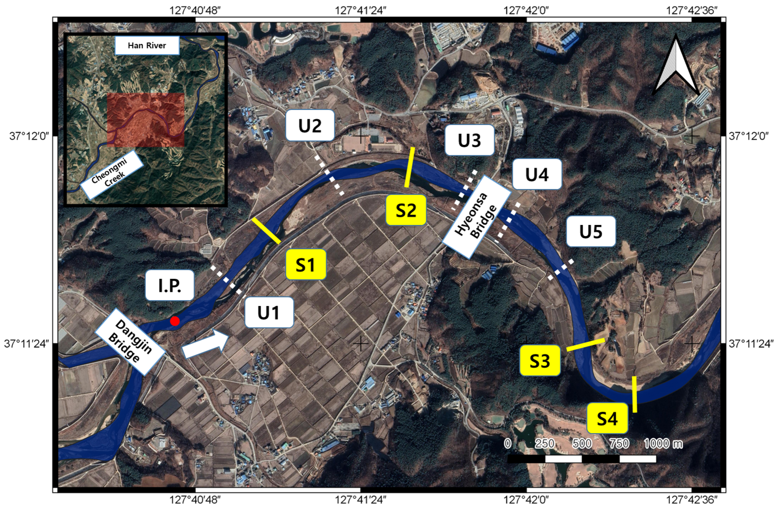
To validate the suggested empirical equations, we used tracer test data, which was obtained from Cheongmi Creek, Yeoju-si, Gyeonggi-do, South Korea, in 2015 [16]. The experimental reach, a braided river with many storage zone areas (e.g., sand bars, meandering channels, and a bridge), was located downstream of Dangjin Bridge near the confluence with the Han River. The total length of the experimental reach was 3550 m, and it was divided into four sections denoted S1–S4 for measurement of concentration and five sections, denoted U1–U5 for measurement of hydraulic properties (Figure 13).
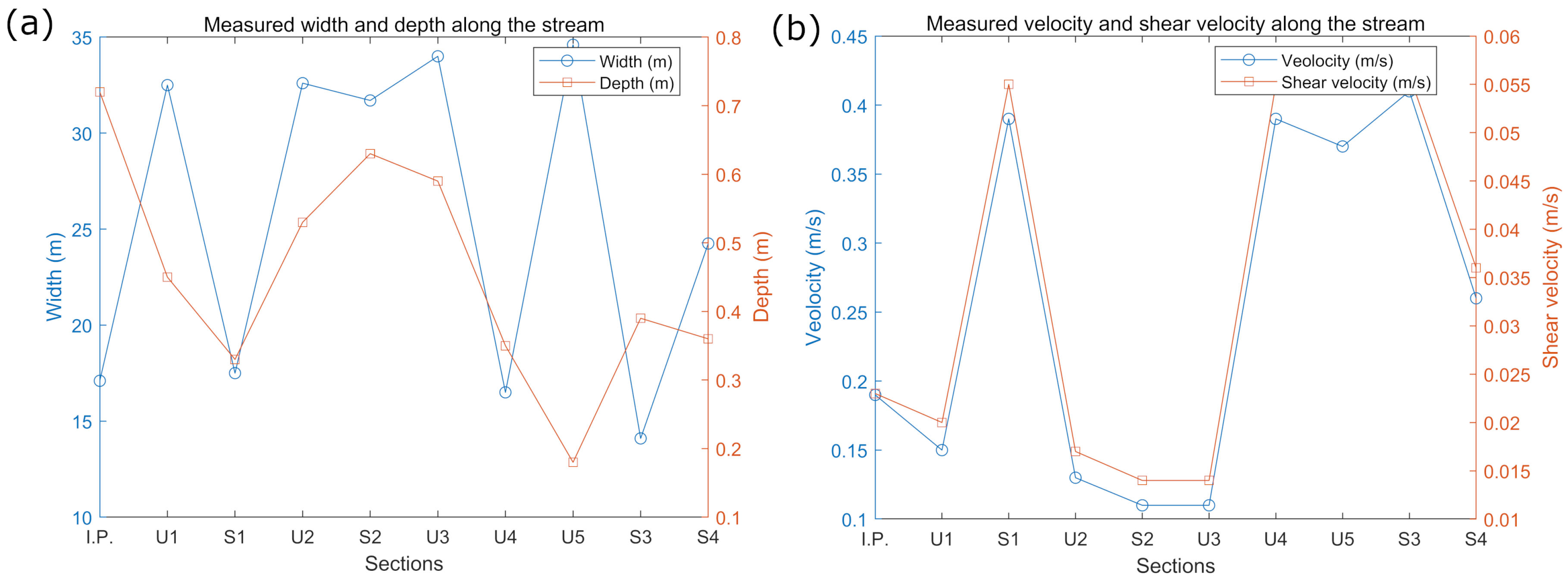
Table 4 and Figure 14 show the hydromorphic properties measured in the Cheongmi Creek tracer test. In the table, is the flow distance from the injection point (IP). The shear velocity had been calculated using the slope from the Manning equation, and the applied Manning coefficient, 0.037, was determined by consulting the published guide [79]. Cross-sectional mean velocity and water depth were measured using RDI-StreamPro ADCP at all sites. The discharge during the tracer test was 2.26 m3/s, and the cross-sectional area was calculated, dividing measured discharge by mean velocity (Table 4). Sinuosity can be calculated with plan view. The calculated sinuosity of the specified reaches S1-S2, S2-S3, and S3-S4 are 1.0562, 1.0671, and 1.1207, respectively.
The experimental site is a meandering channel with sand bars at the inner banks. The meandering bends start at the sub-reaches S1-S2 and S3-S4. In sub-reach S3-S4, the river flows more rapidly and more sinuous than in sub-reach S1-S2. The sub-reach S2-S3 is the downstream half of the first bend where flow accelerates. In addition, The sub-section S2-S3 is the most complicated section due to the Hyeonsa Bridge, which accompanies vortical structure, sudden contraction, and expansion. Therefore, cross-sectional shape and velocity change abruptly between S2 and S3.
Rhodamine WT (RWT) (0.2 kg) was injected at multiple points considering the one-dimensional fully-mixed condition (both horizontally and vertically) in a natural stream. The distance between the IP and S1 can be estimated using Equation (28) [80].
in which, is the distance from the injection point for complete mixing on cross-section [L]; n is the number of injection points in the lateral direction; and is the lateral mixing coefficient which is estimated from [45] []. The fully mixed condition distance from the IP was estimated at 300 m using Equation (28). The distance between IP and S1 was set at 940 m to consider the storage effect in the braided channel, from a conservative perspective.
RWT was measured using YSI-600OMS fluorometers; the measurement devices were calibrated beside the experimental river before being installed. In order to obtain cross-sectional averaged concentrations, three or four sensors were fixed at laterally uniform distances at all measurement sites. During postprocessing, the recorded concentrations were corrected, taking into account stream temperature differences due to the day crossing by referencing the temperature at the start of the observation (Equation (29)) [81]. Also, the background concentration was removed in keeping with the corrected concentration considering the variation in temperature from Equation (29).
where C and are the RWT concentrations at temperatures t and , respectively [ppm]; t is the temperature of the stream during the measurement [°C]; is the reference temperature; and is the temperature calibration coefficient of RWT () [82].
4.2. Simulation Results
In this subsection, TSM parameters and BTCs were predicted using the hydromorphic properties measured with the tracer test. Table 5 summarizes the calibrated TSM parameters via inverse modeling and the TSM parameters calculated using the three empirical models (MGGP, PCR, and F2019). In addition to the TSM parameters, was calculated in each case to assess whether the estimation was reasonable. is given by:
where is the reach length [L]. Every evaluated value was in a range of [0.1 10], which is a reasonable estimation range [62,74]. Since F2019 do not provide a formula for , reach averaged cross-sectional area was adopted instead.
In the sub-reach S1-S2, a sand bar had migrated because of the sudden expansion of the channel. The mean cross-sectional area of the first sub-reach was 14.6009 m2, and the calibrated was smaller than the actual cross-section. The defect of the calibrated contributed 5.4298 m2 to the storage zone area, but was greater than the measured cross-section area due to the sand bar HTS. Moreover, the measured velocity at S1 (0.39 m/s) was more than three times faster than that at U2 (0.13 m/s) and S2 (0.11 m/s), so that the estimate of the effective area was low. Keeping in mind the s value used in the F2019, the MGGP model better predicted than the PCR model, in the sub-reach S1-S2. The F2019 and PCR models over-estimated ; the values in those models were 4.31 times, and 2.5 times higher, respectively. Every model under-estimated the storage parameters ( and ).
The second sub-reach, S2-S3, included the Hyeonsa Bridge, which is an artificial STS. Due to the existence of the bridge pier, hydromorphic variables were extensively altered throughout the reach. Thus, , which reflects the storage effect, was higher in this sub-reach than in other sub-reaches, despite the magnitudes of and being half of those in compared to the reach S1-S2. The MGGP model was superior to F2019 and PCR models in the prediction of the four parameters, while all models over-estimated and under-estimated two storage parameters. The F2019 model predicted as 7.2714, which is six times higher than the calibrated value. The predictabilities of and were reasonable in the order MGGP-F2019-PCR and MGGP-PCR-F2019, respectively.
The last sub-reach, S3-S4, was a meandering band reach with channel expansion. Unlike in the other sub-reaches, in this sub-reach, the measured cross-section was smaller than the calibrated value. Furthermore, using the PCR model for was the best choice in this reach, whereas the measured value was more reliable in the other reaches. In terms of , the MGGP model was most accurate, followed by PCR-F2019. The MGGP model predicted accurately, but F2019 was better at predicting .
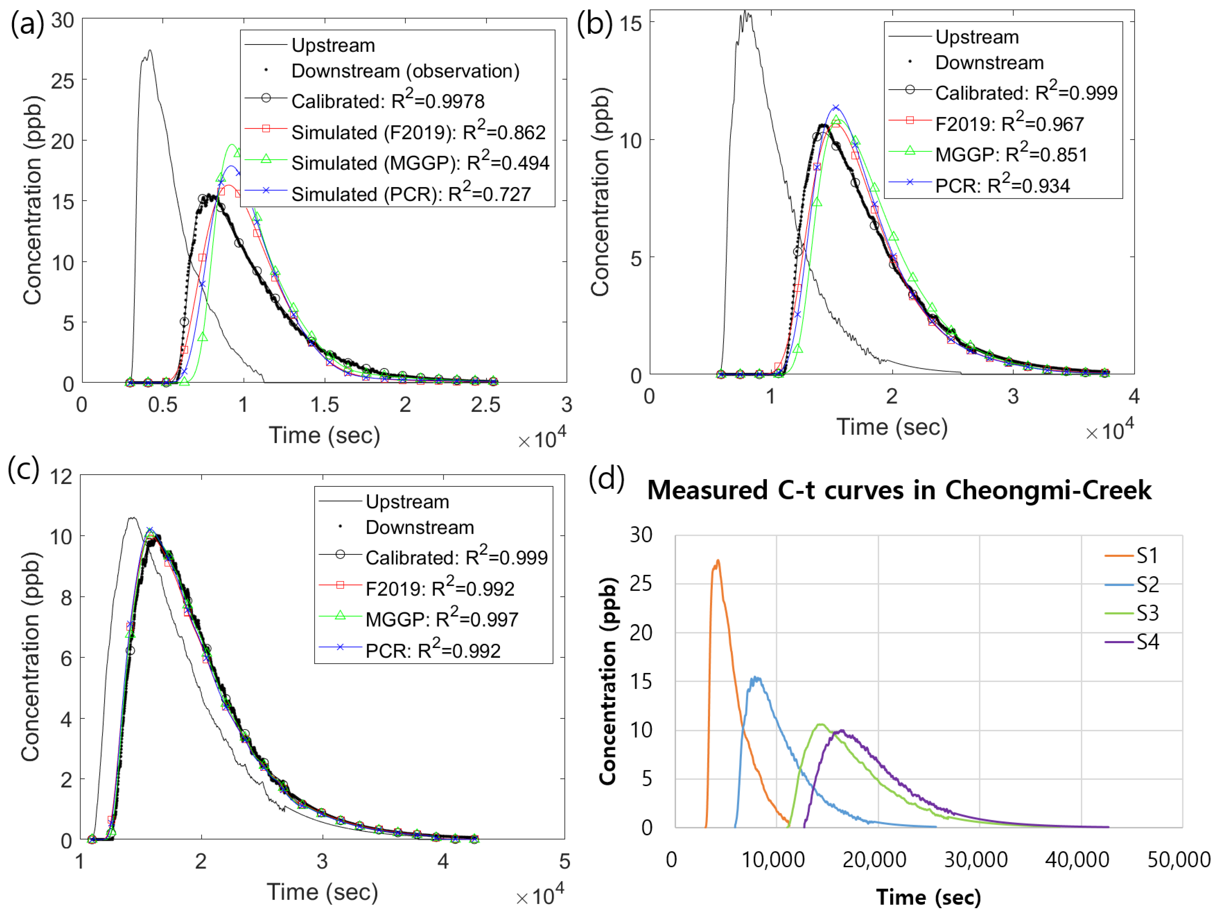
The observed BTCs in the tracer test and the curves generated using the empirical equations are shown in Figure 15. The BTCs in sub-reaches S1-S2 and S2-S3 using the F2019 model had the largest s, followed by the PCR model and MGGP model. In the last sub-reach, the three models produced values with good accuracy, with ; and the of the MGGP BTC was the largest, 0.997.
From the perspective of shape, the BTCs from F2019 had slow rises and steep decreases. The PCR and MGGP models reproduced steep rises and gentle tails. In the first two sub-reaches, S1-S2 and S2-S3, the peaks of the MGGP and PCR BTCs appeared slower than did the BTCs from F2019. Thus the F2019 model simulated the observed BTCs more precisely, even though the MGGP and PCR models predicted , , and more accurately. All models simulated BTCs without a phase lag in the last sub-reach, while all models predicted with high accuracy. This result revealed that precise prediction of significantly affects the production of BTCs, which have accurate time-related features, such as the time to peak concentration, time to centroid, and so on.
Regarding both the estimation values and simulated BTCs, overall predictabilities were high in the order of S3-S4, S2-S3, and S1-S2. Contrary to, , which is given by Equation (7), followed the inverse order of the predictabilities. Especially, the BTCs and TSM parameters in S2-S3 were much successfully estimated than in S1-S2, although -based uncertainty was higher in S2-S3 than in S1-S2. It implies that has a positive correlation with uncertainty in parameter estimation. The largest wetted area (, , , W, and h) and the slowest flow were observed in the first sub-reach, S1-S2, among the sub-reaches. As aforementioned, the TSM is inferior as the ratio HTS has more significance than STS, resulting in problematic prediction. Therefore, it hints that HTS was more influential than STS in the sub-reach S1-S2 since friction factor f and account for the hyporheic exchange particularly [71,83].
5. Sensitivity Analysis
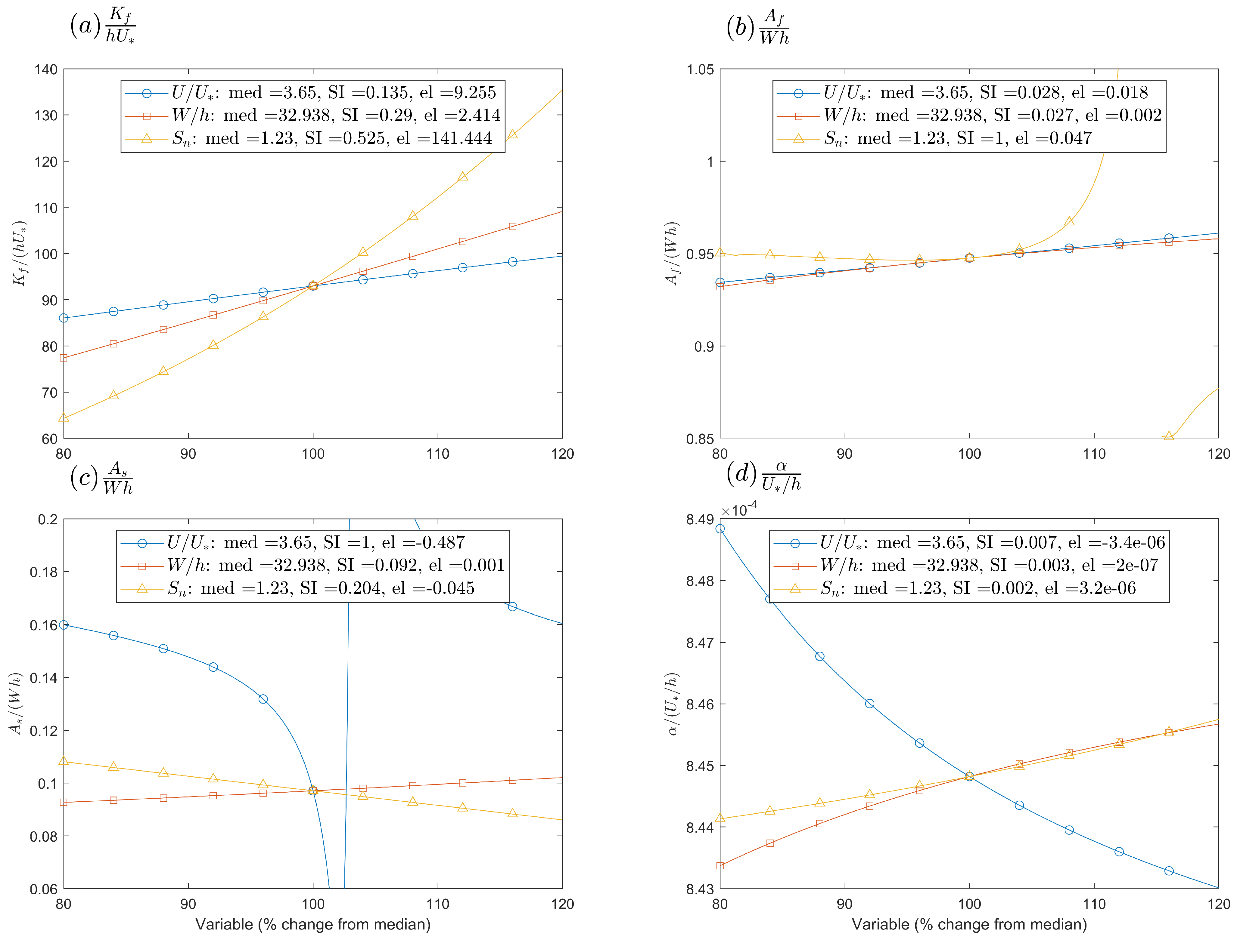
As demonstrated in the preceding sections, the MGGP model stably predicted the TSM parameters. Hence, the MGGP model has been adopted as a benchmark model for the following sensitivity analysis. One-at-a-time (OAT) sensitivity analysis was performed to identify the extent to which a change in the input variable’s of, ±20% from the medians, affect the TSM parameters. For quantitative assessments, the elasticity (Equation (31)) and the sensitivity index (SI) (Equation (32)) were computed.
where is a gradient of the parameter using the median where input variables, and indicates the absolute rate of change when the variable changes by 40%. The magnitude of a variable is reflected in the calculation of , though considers only the targeted parameter.
Figure 16 presents spider plots and two sensitivity indices for each MGGP equation, since the MGGP model showed the highest correlation with our observations in every TSM parameter. Figure 16a shows that is sensitive to which supports previous studies on mixing in meandering channels, in which that sinuosity had a strong positive relationship with secondary current [84,85], increasing the dispersion coefficient [86]. The other dimensionless input variables were also found to increase shear dispersion. The of , 141, was the highest due to the small order, and it is 14 times more significant than the value of . In terms of , is the most sensitive variable, followed by and . The values of and were 0.135 and 0.29, respectively.
On the other hand, the main flow zone area, , was insensitive at low sinuosity, though it was nonlinear at high sinuosity. Thus, the general sensitivity of was not clear despite having the largest and . However, the power of in the PCR model for (Equation (17)) was 0.0729, which is the smallest power, implying that the effect of on is not significant. and yielded similar values, even though was nine times more sensitive than in terms of .
and were reciprocal to the storage zone area, , except for around the median value of which showed nonlinear behavior around the median value. Even though showed nonlinear behavior resulting in very large sensitivity criteria, the absolute power of the PCR equation was 0.6310, which is an intermediate value between that of the other two variables. In the spider plot, the influences of the input variables were significant in the order , , and . Boundary shear stress affects a slow storage zone area in a wide river. In a river with a wide cross-sectional area, there are more likely to be transient storage areas, so a weakly positive correlation of with is established.
Figure 16d shows different features from those of the PCR equation, Equation (19), illustrating that the mass exchange rate is negatively correlated with all input variables. The action of on is most powerful at . However, presented similar elasticity to with and . In total parameter adjustment, was slightly more responsive than ; was in which 0.003 and 0.002, respectively. However, the elasticity of was sixteen times weaker than that of the other hydromorphic variables. This result showed that a change in the exchange rate is mainly governed by since it intensifies the advective effect, and the turbulence intensity in the main flow zone.
From subplots (c) and (d) in Figure 16, as increases, decreases more rapidly than increases. It means that has a negative correlation with . In a similar approach, is proportional to since of in was two times larger than in . This analogy about , the ratio of stream power and friction, in the storage parameters, and , coincides with the observations that the U and f are the most relevant factor [62,71,83].
According to the graphs, the most significant features in the main flow zone dispersion and the storage zone processes are and , respectively. However, we note that the variance of is very small compared to and . Regarding this, the contributions of would be remarkable to both and the transient storage effect. Thus the assumption that is a driving factor in the one-dimensional mixing process is still valid.
6. Conclusions
In the present study, we investigated how hydromorphic parameters interact with TSM parameters by analyzing empirical equations. In the main purpose of analysis, new equations for four TSM parameters (the main flow zone dispersion coefficient (), the main flow zone area (), the storage zone area (), and the storage exchange rate ()) were developed using MGGP and PCR. The newly proposed equations for the TSM parameters consist of dimensionless TSM parameters (, , , and ) and dimensionless input variables (, , and ) which were derived from dimensional analysis. A total of 128 datasets were selected for the derivation of the equations in the meta-analysis. The two presented models and the model published by Femeena et al. were compared using performance criteria. Afterward, field assessment was carried out by matching observed BTCs from Cheongmi Creek and simulated BTCs using the empirical models. Consequently, OAT sensitivity analysis of the MGGP-based TSM parameter empirical equations was performed.
In terms of the performance criteria, the best model was the MGGP model in the training set. Besides, the MGGP model produced superior results as averaging performance criteria of the training set and test set. Next, the PCR model made stable prediction in the test dataset for , , and . The F2019 model kept over-estimating , but it was slightly better than the other two models in the prediction of in the test set. Considering the overall performance indices, the MGGP equations stably predicted all TSM parameters.
The results of the instream application indicated that all empirical models generated acceptable BTCs. However, prediction of mean stream velocity, accounting for , over the complicated reach of a natural stream, using simple methods, remains infeasible.
In the sensitivity analysis section, which focused on the MGGP model, significantly affected . Change in was more responsive to , and . The effect of on was considerable compared to the effects of the other dimensionless variables. The exchange rate, , was mostly affected by the ratio of stream velocity and shear velocity, .
Regardless of the applicability of the developed equations, hidden relationships of non-applied features of the transient storage effect may have been neglected in this study, since the adopted hydromorphic variables were insufficient to explain the complicated storage zones in real rivers. Nevertheless, we suggest the use of the new empirical equations to analyze TSM parameters as reference values in conventional inverse modeling or as an alternate approach in situations where direct inverse modeling is not accessible.
Supplementary Materials
The raw metadata file and MATLAB function files are available online at https://www.mdpi.com/2073-4441/13/1/76/s1.
Author Contributions
Conceptualization, H.N. and I.W.S.; methodology, H.N.; software, H.N.; validation, H.N., I.W.S. and S.K.; formal analysis, H.N.; investigation, H.N.; resources, H.N., S.H.J., D.B. and S.K.; data curation, H.N., S.H.J., D.B. and S.K.; writing—original draft preparation, H.N. and S.K.; writing—review and editing, H.N., I.W.S. and S.K.; visualization, H.N.; supervision, I.W.S.; project administration, I.W.S.; funding acquisition, I.W.S. All authors have read and agreed to the published version of the manuscript.
Funding
This research was partially supported by the BK21 PLUS research program of the National Research Foundation of Korea, and the Korea Agency for Infrastructure Technology Advancement(KAIA) grant funded by the Ministry of Land, Infrastructure and Transport (Grant 19DPIW-C153746-01).
Institutional Review Board Statement
Not applicable.
Informed Consent Statement
Not applicable.
Data Availability Statement
The data presented in this study are available in https://www.mdpi.com/2073-4441/13/1/76/s1.
Acknowledgments
This research work was conducted at the Institute of Engineering Research and Institute of Construction and Environmental Engineering in Seoul National University, Seoul, Korea. We wish to thank P.V. Femeena for providing supplementary data used to derive TSM models in their study.
Conflicts of Interest
The authors declare no conflict of interest.
Abbreviations
The following abbreviations are used in this manuscript:
| 1D-ADE | 1-Dimension Advection-Dispersion Equation |
| BTC | Breakthrough Curve |
| DR | Discrepancy Ratio |
| GA | Genetic Algorithm |
| GP | Genetic Programming |
| HTS | Hyporheic Transient Storage |
| MGGP | Multi-Gene Genetic Programming |
| MSE | Mean Squared Error |
| MSL | Mean Sea Level |
| OAT | One-At-a-Time |
| OTIS | One-Dimensional Transport with Inflow and Storage |
| PCR | Principal Components Regression |
| RMSE | Root Mean Squared Error |
| RTD | Residence Time Distribution |
| RWT | Rhodamine WT |
| SC-SAHEL | Shuffled Complex-Self Adaptive EvoLution |
| SCE-UA | Shuffled Complex Evolution-University of Arizona |
| SI | Sensitivity Index |
| STS | Surface Transient Storage |
| TSM | Transient Storage Model |
| VIF | Variance Inflation Factor |
Appendix A. Description of the Gam-Creek Tracer Test
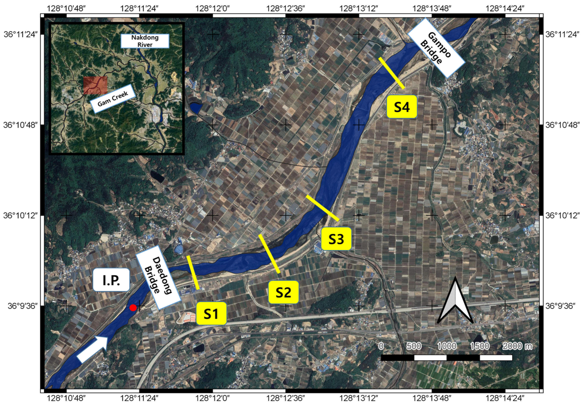
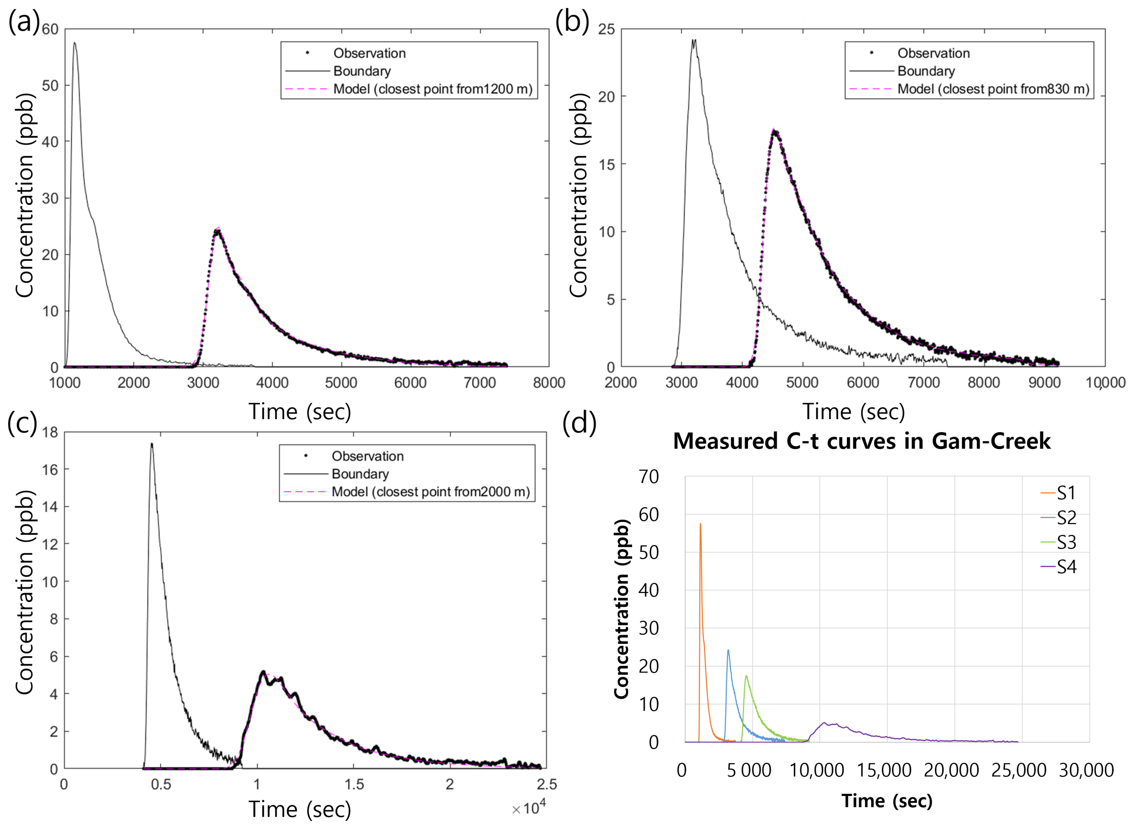
Additional tracer test was performed in Gam-Creek, Gimcheon-si, Gyeongsangbuk-do to collect the calibrated TSM parameters. Figure A1 and Figure A2 show the plan view and obtained BTCs, respectively, in the tracer test. A bathymetry survey was conducted utilizing Real-Time Kinematic-Global Positioning System (RTK-GPS). The used RTK-GPS model is Sokkia GRX1. The used coordinate of the GPS is a GSR80 ellipsoid Traverse Mercator X-Y type (EPSG: 5186), which is a standard of the National Geographic Information Institute of Korea. Sontek FlowTracker and YSI-600OMS fluorometers are used to measure flow velocity and BTCs. The calibrated TSM parameters and the measured hydromorphic variables are showed in Table A1.
Figure A1.
Plan view of the Gam-Creek tracer test.

Figure A2.
Observed BTCs in Gam-Creek tracer test and calibrated BTCs; (a) section 1–2. (b) section 2–3. (c) section 3–4. (d) All stations (only meausred curves).
Figure A2.
Observed BTCs in Gam-Creek tracer test and calibrated BTCs; (a) section 1–2. (b) section 2–3. (c) section 3–4. (d) All stations (only meausred curves).


Table A1.
Measured hydraulic features and estimated TSM parameters in the Gam-Creek tracer test.
| Variables | Reach | |||
|---|---|---|---|---|
| S1-S2 | S2-S3 | S3-S4 | ||
| Hydraulic Features | (m) | 1200 | 830 | 2000 |
| Q (cms) | 11.06 | 11.06 | 11.06 | |
| W (m) | 57.36 | 58.86 | 53.00 | |
| h (m) | 0.36 | 0.36 | 0.43 | |
| 0.0007 | 0.0024 | 0.0007 | ||
| (m/s) | 0.53 | 0.52 | 0.48 | |
| 1.082 | 1.028 | 1.078 | ||
| TSM Parameters | 0.568 | 0.596 | 4.926 | |
| 18.279 | 17.175 | 31.135 | ||
| 4.1473 | 2.6932 | 10.4883 | ||
| (1/s) | 3.758 | 2.920 | 1.533 | |
Appendix B. Derived PCR Equations Using Total Dataset
The below PCR-based equations derived using the total dataset are provided for those who want to use them in expanded use.
References
- Fischer, H.B.; Brooks, N.H. Longitudinal Dispersion in Laboratory and Natural Streams; Tecnical Report No. KH-R-12; California Institute of Technology, W. M. Keck Laboratory of Hydraulics and Water Resources: Pasadena, CA, USA, 1966. [Google Scholar]
- Hays, J.R. Mass Transport Mechanisms in Open Channel Flow. Ph.D. Thesis, Vanderbilt University, Nashville, TN, USA, 1967. [Google Scholar]
- Day, T.J. Longitudinal dispersion in natural channels. Water Resour. Res. 1975, 11, 909–918. [Google Scholar] [CrossRef]
- Pederson, F. Prediction of Longitudinal Dispersion in Natural Streams; Technical Report Series Paper 14; Technical University of Denmark: Lyngby, Denmark, 1977. [Google Scholar]
- Beltaos, S.; Day, T. A field study of longitudinal dispersion. Can. J. Civ. Eng. 1978, 5, 572–585. [Google Scholar] [CrossRef]
- Sabol, G.V.; Nordin, C.F. Dispersion in rivers as related to storage zones. J. Hydraul. Div. 1978, 104, 695–708. [Google Scholar]
- Liu, H.; Cheng, A.H. Modified Fickian model for predicting dispersion. J. Hydraul. Div. 1980, 106, 1021–1040. [Google Scholar]
- Chatwin, P.C. Presentation of longitudinal dispersion data. J. Hydraul. Div. 1980, 106, 71–83. [Google Scholar]
- Beer, T.; Young, P.C. Longitudinal dispersion in natural streams. J. Environ. Eng. 1983, 109, 1049–1067. [Google Scholar] [CrossRef]
- Bencala, K.E. Simulation of solute transport in a mountain pool-and-riffle stream with a kinetic mass transfer model for sorption. Water Resour. Res. 1983, 19, 732–738. [Google Scholar] [CrossRef]
- Abbe, T.B.; Montgomery, D.R. Large woody debris jams, channel hydraulics and habitat formation in large rivers. Regul. Rivers Res. Manag. 1996, 12, 201–221. [Google Scholar] [CrossRef]
- Abbe, T.B.; Montgomery, D.R. Patterns and processes of wood debris accumulation in the Queets river basin, Washington. Geomorphology 2003, 51, 81–107. [Google Scholar] [CrossRef]
- Tonina, D.; Buffington, J.M. Hyporheic exchange in mountain rivers I: Mechanics and environmental effects. Geogr. Compass 2009, 3, 1063–1086. [Google Scholar] [CrossRef]
- Nepf, H.M. Flow and transport in regions with aquatic vegetation. Annu. Rev. Fluid Mech. 2012, 44, 123–142. [Google Scholar] [CrossRef] [Green Version]
- Jackson, T.R.; Haggerty, R.; Apte, S.V. A fluid-mechanics based classification scheme for surface transient storage in riverine environments: Quantitatively separating surface from hyporheic transient storage. Hydrol. Earth Syst. Sci. 2013, 17, 2747–2779. [Google Scholar] [CrossRef] [Green Version]
- Noh, H.; Baek, D.; Seo, I.W. Analysis of the applicability of parameter estimation methods for a transient storage model. J. Korea Water Resour. Assoc. 2019, 52, 681–695. [Google Scholar]
- Boano, F.; Harvey, J.W.; Marion, A.; Packman, A.I.; Revelli, R.; Ridolfi, L.; Wörman, A. Hyporheic flow and transport processes: Mechanisms, models, and biogeochemical implications. Rev. Geophys. 2014, 52, 603–679. [Google Scholar] [CrossRef]
- Choi, J.; Harvey, J.W.; Conklin, M.H. Characterizing multiple timescales of stream and storage zone interaction that affect solute fate and transport in streams. Water Resour. Res. 2000, 36, 1511–1518. [Google Scholar] [CrossRef]
- Deng, Z.Q.; Singh, V.P.; Bengtsson, L. Numerical solution of fractional advection-dispersion equation. J. Hydraul. Eng. 2004, 130, 422–431. [Google Scholar] [CrossRef] [Green Version]
- Singh, S.K. Treatment of stagnant zones in riverine advection-dispersion. J. Hydraul. Eng. 2003, 129, 470–473. [Google Scholar] [CrossRef]
- Haggerty, R.; McKenna, S.A.; Meigs, L.C. On the late-time behavior of tracer test breakthrough curves. Water Resour. Res. 2000, 36, 3467–3479. [Google Scholar] [CrossRef] [Green Version]
- Wörman, A.; Packman, A.I.; Johansson, H.; Jonsson, K. Effect of flow-induced exchange in hyporheic zones on longitudinal transport of solutes in streams and rivers. Water Resour. Res. 2002, 38. [Google Scholar] [CrossRef] [Green Version]
- Boano, F.; Packman, A.; Cortis, A.; Revelli, R.; Ridolfi, L. A continuous time random walk approach to the stream transport of solutes. Water Resour. Res. 2007, 43. [Google Scholar] [CrossRef]
- Marion, A.; Zaramella, M. A residence time model for stream-subsurface exchange of contaminants. Acta Geophys. Pol. 2005, 53, 527. [Google Scholar]
- Davis, P.; Atkinson, T. Longitudinal dispersion in natural channels: 3. An aggregated dead zone model applied to the River Severn, UK. Hydrol. Earth Syst. SC 2000, 4, 373–381. [Google Scholar] [CrossRef]
- Runkel, R.L. One-Dimensional Transport with Inflow and Storage (OTIS): A Solute Transport Model for Streams and Rivers; US Department of the Interior, US Geological Survey: Washington, DC, USA, 1998; Volume 98.
- Kelleher, C.; Wagener, T.; McGlynn, B.; Ward, A.; Gooseff, M.; Payn, R. Identifiability of transient storage model parameters along a mountain stream. Water Resour. Res. 2013, 49, 5290–5306. [Google Scholar] [CrossRef]
- Ward, A.S.; Kelleher, C.A.; Mason, S.J.; Wagener, T.; McIntyre, N.; McGlynn, B.; Runkel, R.L.; Payn, R.A. A software tool to assess uncertainty in transient-storage model parameters using Monte Carlo simulations. Freshw. Sci. 2017, 36, 195–217. [Google Scholar] [CrossRef] [Green Version]
- Wagner, B.J.; Harvey, J.W. Experimental design for estimating parameters of rate-limited mass transfer: Analysis of stream tracer studies. Water Resour. Res. 1997, 33, 1731–1741. [Google Scholar] [CrossRef] [Green Version]
- Choi, S.Y.; Seo, I.W.; Kim, Y.O. Parameter uncertainty estimation of transient storage model using Bayesian inference with formal likelihood based on breakthrough curve segmentation. Environ. Model. Softw. 2020, 123, 104558. [Google Scholar] [CrossRef]
- Wallis, S.; Manson, R. Sensitivity of optimized transient storage model parameters to spatial and temporal resolution. Acta Geophys. 2019, 67, 951–960. [Google Scholar] [CrossRef] [Green Version]
- Boano, F.; Revelli, R.; Ridolfi, L. Source identification in river pollution problems: A geostatistical approach. Water Resour. Res. 2005, 41. [Google Scholar] [CrossRef]
- Ghane, A.; Mazaheri, M.; Samani, J.M.V. Location and release time identification of pollution point source in river networks based on the backward probability method. J. Environ. Manag. 2016, 180, 164–171. [Google Scholar] [CrossRef]
- Zhang, S.P.; Xin, X.K. Pollutant source identification model for water pollution incidents in small straight rivers based on genetic algorithm. Appl. Water Sci. 2017, 7, 1955–1963. [Google Scholar] [CrossRef] [Green Version]
- Thackston, E.L.; Schnelle, K.B. Predicting effects of dead zones on stream mixing. J. Sanit. Eng. Div. 1970, 96, 319–331. [Google Scholar]
- Seo, I.W.; Yu, D.Y. Characterization of pool-riffle sequences in solute transport modeling of streams. Water Eng. Res. 2000, 1, 171–185. [Google Scholar]
- Cheong, T.S.; Seo, I.W. Parameter estimation of the transient storage model by a routing method for river mixing processes. Water Resour. Res. 2003, 39. [Google Scholar] [CrossRef]
- Cheong, T.S.; Younis, B.A.; Seo, I.W. Estimation of key parameters in model for solute transport in rivers and streams. Water Resour. Manag. 2007, 21, 1165–1186. [Google Scholar] [CrossRef]
- Sahay, R.R. Predicting transient storage model parameters of rivers by genetic algorithm. Water Resour. Manag. 2012, 26, 3667–3685. [Google Scholar] [CrossRef]
- Femeena, P.; Chaubey, I.; Aubeneau, A.; McMillan, S.; Wagner, P.; Fohrer, N. Simple regression models can act as calibration-substitute to approximate transient storage parameters in streams. Adv. Water Resour. 2019, 123, 201–209. [Google Scholar] [CrossRef]
- Riahi-Madvar, H.; Dehghani, M.; Seifi, A.; Singh, V.P. Pareto Optimal Multigene Genetic Programming for Prediction of Longitudinal Dispersion Coefficient. Water Resour. Manag. 2019, 33, 905–921. [Google Scholar] [CrossRef]
- Taylor, G.I. The dispersion of matter in turbulent flow through a pipe. Proc. R. Soc. London. Ser. A Math. Phys. Sci. 1954, 223, 446–468. [Google Scholar]
- Elder, J. The dispersion of marked fluid in turbulent shear flow. J. Fluid Mech. 1959, 5, 544–560. [Google Scholar] [CrossRef]
- McQuivey, R.S.; Keefer, T.N. Simple method for predicting dispersion in streams. J. Environ. Eng. Div. 1974, 100, 997–1011. [Google Scholar]
- Fischer, H.B.; List, J.E.; Koh, C.R.; Imberger, J.; Brooks, N.H. Mixing in Inland and Coastal Waters; Elsevier: Amsterdam, The Netherlands, 2013. [Google Scholar]
- Seo, I.W.; Cheong, T.S. Predicting longitudinal dispersion coefficient in natural streams. J. Hydraul. Eng. 1998, 124, 25–32. [Google Scholar] [CrossRef]
- Kashefipour, S.M.; Falconer, R.A. Longitudinal dispersion coefficients in natural channels. Water Res. 2002, 36, 1596–1608. [Google Scholar] [CrossRef]
- Disley, T.; Gharabaghi, B.; Mahboubi, A.; McBean, E. Predictive equation for longitudinal dispersion coefficient. Hydrol. Process. 2015, 29, 161–172. [Google Scholar] [CrossRef]
- Alizadeh, M.J.; Ahmadyar, D.; Afghantoloee, A. Improvement on the existing equations for predicting longitudinal dispersion coefficient. Water Resour. Manag. 2017, 31, 1777–1794. [Google Scholar] [CrossRef]
- Mehr, A.D.; Kahya, E. A Pareto-optimal moving average multigene genetic programming model for daily streamflow prediction. J. Hydrol. 2017, 549, 603–615. [Google Scholar] [CrossRef]
- Valencia-Ramírez, J.M.; Raya, J.A.; Cedeno, J.R.; Suárez, R.R.; Escalante, H.J.; Graff, M. Comparison between Genetic Programming and full model selection on classification problems. In Proceedings of the 2014 IEEE International Autumn Meeting on Power, Electronics and Computing (ROPEC), Ixtapa, Mexico, 5–7 November 2014; pp. 1–6. [Google Scholar]
- Gandomi, A.H.; Sajedi, S.; Kiani, B.; Huang, Q. Genetic programming for experimental big data mining: A case study on concrete creep formulation. Autom. Constr. 2016, 70, 89–97. [Google Scholar] [CrossRef] [Green Version]
- Chatwin, P.; Allen, C. Mathematical models of dispersion in rivers and estuaries. Annu. Rev. Fluid Mech. 1985, 17, 119–149. [Google Scholar] [CrossRef]
- Valentine, E.M.; Wood, I.R. Longitudinal dispersion with dead zones. J. Hydraul. Div. 1977, 103, 975–990. [Google Scholar]
- Hart, D.R. Parameter estimation and stochastic interpretation of the transient storage model for solute transport in streams. Water Resour. Res. 1995, 31, 323–328. [Google Scholar] [CrossRef]
- Bottacin-Busolin, A.; Marion, A.; Musner, T.; Tregnaghi, M.; Zaramella, M. Evidence of distinct contaminant transport patterns in rivers using tracer tests and a multiple domain retention model. Adv. Water Resour. 2011, 34, 737–746. [Google Scholar] [CrossRef]
- Haggerty, R.; Wondzell, S.M.; Johnson, M.A. Power-law residence time distribution in the hyporheic zone of a 2nd-order mountain stream. Geophys. Res. Lett. 2002, 29. [Google Scholar] [CrossRef] [Green Version]
- Gooseff, M.N.; Wondzell, S.M.; Haggerty, R.; Anderson, J. Comparing transient storage modeling and residence time distribution (RTD) analysis in geomorphically varied reaches in the Lookout Creek basin, Oregon, USA. Adv. Water Resour. 2003, 26, 925–937. [Google Scholar] [CrossRef]
- Jonsson, K.; Johansson, H.; Wörman, A. Hyporheic exchange of reactive and conservative solutes in streams—Tracer methodology and model interpretation. J. Hydrol. 2003, 278, 153–171. [Google Scholar] [CrossRef]
- Jonsson, K.; Johansson, H.; Wörman, A. Sorption behavior and long-term retention of reactive solutes in the hyporheic zone of streams. J. Environ. Eng. 2004, 130, 573–584. [Google Scholar] [CrossRef]
- Gooseff, M.N.; Hall, R.O., Jr.; Tank, J.L. Relating transient storage to channel complexity in streams of varying land use in Jackson Hole, Wyoming. Water Resour. Res. 2007, 43. [Google Scholar] [CrossRef]
- Harvey, J.W.; Conklin, M.H.; Koelsch, R.S. Predicting changes in hydrologic retention in an evolving semi-arid alluvial stream. Adv. Water Resour. 2003, 26, 939–950. [Google Scholar] [CrossRef]
- Ensign, S.H.; Doyle, M.W. In-channel transient storage and associated nutrient retention: Evidence from experimental manipulations. Limnol. Oceanogr. 2005, 50, 1740–1751. [Google Scholar] [CrossRef] [Green Version]
- Bukaveckas, P.A. Effects of channel restoration on water velocity, transient storage, and nutrient uptake in a channelized stream. Environ. Sci. Technol. 2007, 41, 1570–1576. [Google Scholar] [CrossRef]
- Rowiński, P.M.; Guymer, I.; Kwiatkowski, K. Response to the slug injection of a tracer—A large-scale experiment in a natural river/Réponse à l’injection impulsionnelle d’un traceur—Expérience à grande échelle en rivière naturelle. Hydrol. Sci. J. 2008, 53, 1300–1309. [Google Scholar] [CrossRef] [Green Version]
- Stofleth, J.M.; Shields, F.D., Jr.; Fox, G.A. Hyporheic and total transient storage in small, sand-bed streams. Hydrol. Process. Int. J. 2008, 22, 1885–1894. [Google Scholar] [CrossRef]
- Guecker, B.; Boechat, I.G.; Giani, A. Impacts of agricultural land use on ecosystem structure and whole-stream metabolism of tropical Cerrado streams. Freshw. Biol. 2009, 54, 2069–2085. [Google Scholar] [CrossRef]
- Claessens, L.; Tague, C.L.; Groffman, P.M.; Melack, J.M. Longitudinal assessment of the effect of concentration on stream N uptake rates in an urbanizing watershed. Biogeochemistry 2010, 98, 63–74. [Google Scholar] [CrossRef] [Green Version]
- Claessens, L.; Tague, C.L.; Groffman, P.M.; Melack, J.M. Longitudinal and seasonal variation of stream N uptake in an urbanizing watershed: Effect of organic matter, stream size, transient storage and debris dams. Biogeochemistry 2010, 98, 45–62. [Google Scholar] [CrossRef] [Green Version]
- Stonedahl, S.H.; Harvey, J.W.; Detty, J.; Aubeneau, A.; Packman, A.I. Physical controls and predictability of stream hyporheic flow evaluated with a multiscale model. Water Resour. Res. 2012, 48. [Google Scholar] [CrossRef] [Green Version]
- Johnson, Z.C.; Warwick, J.J.; Schumer, R. Factors affecting hyporheic and surface transient storage in a western US river. J. Hydrol. 2014, 510, 325–339. [Google Scholar] [CrossRef]
- Mueller Price, J.; Baker, D.; Bledsoe, B. Effects of passive and structural stream restoration approaches on transient storage and nitrate uptake. River Res. Appl. 2016, 32, 1542–1554. [Google Scholar] [CrossRef]
- TT Le, A.; Kasahara, T.; Vudhivanich, V. Seasonal Variation and Retention of Ammonium in Small Agricultural Streams in Central Thailand. Environments 2018, 5, 78. [Google Scholar] [CrossRef] [Green Version]
- Bohrman, K.J.; Strauss, E.A. Macrophyte-driven transient storage and phosphorus uptake in a western Wisconsin stream. Hydrol. Process. 2018, 32, 253–263. [Google Scholar] [CrossRef]
- Naeini, M.R.; Yang, T.; Sadegh, M.; AghaKouchak, A.; Hsu, K.l.; Sorooshian, S.; Duan, Q.; Lei, X. Shuffled Complex-Self Adaptive Hybrid EvoLution (SC-SAHEL) optimization framework. Environ. Model. Softw. 2018, 104, 215–235. [Google Scholar] [CrossRef] [Green Version]
- Searson, D.P. GPTIPS 2: An open-source software platform for symbolic data mining. In Handbook of Genetic Programming Applications; Springer: Berlin/Heidelberg, Germany, 2015; pp. 551–573. [Google Scholar]
- Verboven, S.; Hubert, M. LIBRA: A MATLAB library for robust analysis. Chemom. Intell. Lab. Syst. 2005, 75, 127–136. [Google Scholar] [CrossRef]
- Memarzadeh, R.; Zadeh, H.G.; Dehghani, M.; Riahi-Madvar, H.; Seifi, A.; Mortazavi, S.M. A novel equation for longitudinal dispersion coefficient prediction based on the hybrid of SSMD and whale optimization algorithm. Sci. Total. Environ. 2020, 716, 137007. [Google Scholar] [CrossRef] [PubMed]
- Arcement, G.J.; Schneider, V.R. Guide for Selecting Manning’s Roughness Coefficients for Natural Channels and Flood Plains; Water-Resource Paper 2339; U.S. Geological Survey: Washington, DC, USA, 1989.
- Kilpatrick, F.A.; Wilson, J.F. Measurement of Time of Travel in Streams by Dye Tracing; Chapter A9, USGS Techniques of Water-Resources Investigations; U.S. Geological Survey: Washington, DC, USA, 1989; Volume 3.
- Jin, L.; Siegel, D.I.; Lautz, L.K.; Otz, M.H. Transient storage and downstream solute transport in nested stream reaches affected by beaver dams. Hydrol. Process. Int. J. 2009, 23, 2438–2449. [Google Scholar] [CrossRef]
- Smart, P.; Smith, D. Water tracing in tropical regions, the use of fluorometric techniques in Jamaica. J. Hydrol. 1976, 30, 179–195. [Google Scholar] [CrossRef]
- Zarnetske, J.P.; Gooseff, M.N.; Brosten, T.R.; Bradford, J.H.; McNamara, J.P.; Bowden, W.B. Transient storage as a function of geomorphology, discharge, and permafrost active layer conditions in Arctic tundra streams. Water Resour. Res. 2007, 43. [Google Scholar] [CrossRef] [Green Version]
- Seo, I.W.; Jung, Y.J. Velocity distribution of secondary currents in curved channels. J. Hydrodyn. Ser. B 2010, 22, 617–622. [Google Scholar] [CrossRef]
- Han, E.J.; Kim, Y.D.; Baek, K.O.; Seo, I.W. Relation between transverse dispersion and diffusion at meandering channel in two-dimensional mixing based on tracer tests. Environ. Earth Sci. 2019, 78, 712. [Google Scholar] [CrossRef]
- Baek, K.O.; Seo, I.W.; Jeong, S.J. Evaluation of dispersion coefficients in meandering channels from transient tracer tests. J. Hydraul. Eng. 2006, 132, 1021–1032. [Google Scholar] [CrossRef]
Figure 1.
Schematics of the surface, hyporheic transient storage zones in an alluvial valley (modified after [11,12,13,14,15]).

Figure 2.
Calibrated BTCs of Cheongmi Creek experiment data from [16] using 1D-ADE and TSM.
Figure 2.
Calibrated BTCs of Cheongmi Creek experiment data from [16] using 1D-ADE and TSM.

Figure 3.
Conceptual diagram of TSM for conservative pollutants.

Figure 4.
Mutation operation of GP.

Figure 5.
Crossover operation of GP.

Figure 6.
Example of MGGP tree structure.

Figure 7.
Boxplots of dimensionless variables; (a) (b) (c) (d) . (e) . (f) . (g) .

Figure 8.
Scree plot of principal components.

Figure 9.
Observed parameter values versus predicted values by empirical equations for the training set; (a) . (b) . (c) . (d) .
Figure 9.
Observed parameter values versus predicted values by empirical equations for the training set; (a) . (b) . (c) . (d) .

Figure 10.
Observed parameter values versus predicted values by empirical equations for the test set; (a) . (b) . (c) . (d) .
Figure 10.
Observed parameter values versus predicted values by empirical equations for the test set; (a) . (b) . (c) . (d) .

Figure 11.
DR histograms of each empirical equations for TSM parameters for the training set; (a) . (b) . (c) . (d) .
Figure 11.
DR histograms of each empirical equations for TSM parameters for the training set; (a) . (b) . (c) . (d) .

Figure 12.
DR histograms of each empirical equations for TSM parameters for the test set; (a) . (b) . (c) . (d) .
Figure 12.
DR histograms of each empirical equations for TSM parameters for the test set; (a) . (b) . (c) . (d) .

Figure 13.
Plan view of the Cheongmi Creek test site.

Figure 14.
Plots of measured hydraulic data in Cheong-mi Creek; (a) Width and depth; (b) Velocity and shear velocity.
Figure 14.
Plots of measured hydraulic data in Cheong-mi Creek; (a) Width and depth; (b) Velocity and shear velocity.

Figure 15.
Simulated and observed breakthrough curves in Cheongmi Creek experiment case: (a) section 1–2. (b) section 2–3. (c) section 3–4. (d) All stations (only measured curves).
Figure 15.
Simulated and observed breakthrough curves in Cheongmi Creek experiment case: (a) section 1–2. (b) section 2–3. (c) section 3–4. (d) All stations (only measured curves).

Figure 16.
Spider plots and calculated indices for sensitivity analysis of the MGGP model; (a) . (b) . (c) . (d) .
Figure 16.
Spider plots and calculated indices for sensitivity analysis of the MGGP model; (a) . (b) . (c) . (d) .

Table 1.
Statistics of the transient storage parameters.
| Parameter | Training Set (90 Sets) | Test Set (38 Sets) | ||||
|---|---|---|---|---|---|---|
| Mean | Minimum | Maximum | Mean | Minimum | Maximum | |
| 46.83 | 3.80 | 331.86 | 36.51 | 3.80 | 114.51 | |
| 5.07 | 1.02 | 17.59 | 5.20 | 1.02 | 15.58 | |
| 1.36 | 1.00 | 2.27 | 1.34 | 1.00 | 2.00 | |
| 335.26 | 0.60 | 5558.20 | 295.79 | 3.42 | 1841.00 | |
| 1.02 | 0.26 | 7.00 | 1.01 | 0.47 | 2.78 | |
| 0.22 | 0.00 | 3.09 | 0.14 | 0.01 | 0.44 | |
| 19.50 | 0.04 | 256.80 | 14.14 | 0.34 | 164.99 | |
Table 2.
MGGP parameter settings.
| Parameter | Settings |
|---|---|
| Function set | , square, cube, exp, tanh, power |
| Population size | 500 |
| Number of generations | 500 |
| Runs | over 200 |
| Maximum number of genes allowed in an individual | 4 |
| Maximum tree depth | 6 |
| Tournament size | 15 |
| Elitism | 0.01 % of population |
| Crossover events | 0.84 |
| High level crossover | 0.2 |
| Low level crossover | 0.8 |
| Mutation events | 0.14 |
| Sub-tree mutation | 0.9 |
| Replacing input terminal with another random terminal | 0.05 |
Table 3.
Calculated performance criteria of empirical equations.
| Criteria | TSM Parameter | Training Set (90 Sets) | Test Set (38 Sets) | ||||
|---|---|---|---|---|---|---|---|
| MGGP | PCR | F2019 | MGGP | PCR | F2019 | ||
| Accuracy (%) | 53.33 | 41.11 | 46.67 | 47.37 | 42.11 | 42.11 | |
| 95.56 | 92.22 | - | 97.37 | 97.37 | - | ||
| 56.67 | 57.78 | 56.67 | 47.37 | 52.63 | 47.37 | ||
| 36.67 | 34.44 | 34.44 | 21.05 | 28.95 | 28.95 | ||
| RMSE | 28.20 | 83.04 | 475.91 | 75.83 | 32.00 | 43.80 | |
| 345.60 | 391.75 | - | 56.92 | 44.86 | - | ||
| 41.96 | 44.80 | 21.43 | 9.54 | 2.60 | 10.58 | ||
| 8.52 | 14.63 | 15.74 | 10.34 | 8.67 | 8.46 | ||
| 0.49 | −3.42 | −144.06 | 0.20 | 0.86 | 0.73 | ||
| 0.93 | 0.91 | - | 0.84 | 0.90 | - | ||
| −0.07 | −0.21 | 0.72 | −3.34 | 0.68 | −4.34 | ||
| 0.67 | 0.04 | −0.11 | −0.29 | 0.09 | 0.14 | ||
| 0.89 | 0.78 | 0.74 | 0.47 | 0.96 | 0.96 | ||
| 0.99 | 0.99 | - | 0.92 | 0.96 | - | ||
| 0.62 | 0.61 | 0.89 | 0.97 | 0.97 | 0.62 | ||
| 0.83 | 0.32 | 0.08 | 0.35 | 0.48 | 0.55 | ||
Table 4.
Measured hydromorphic properties in Cheongmi Creek experiment.
| Station | (m) | W (m) | h (m) | U (m/s) | (m/s) |
|---|---|---|---|---|---|
| I.P | 0 | 17.1 | 0.72 | 0.19 | 0.023 |
| U1 | 380 | 32.5 | 0.45 | 0.15 | 0.020 |
| S1 | 940 | 17.5 | 0.33 | 0.39 | 0.055 |
| U2 | 1300 | 32.6 | 0.53 | 0.13 | 0.017 |
| S2 | 1690 | 31.7 | 0.63 | 0.11 | 0.014 |
| U3 | 2050 | 34 | 0.59 | 0.11 | 0.014 |
| U4 | 2410 | 16.5 | 0.35 | 0.39 | 0.055 |
| U5 | 2730 | 34.6 | 0.18 | 0.37 | 0.057 |
| S3 | 3080 | 14.1 | 0.39 | 0.41 | 0.056 |
| S4 | 3550 | 24.25 | 0.36 | 0.26 | 0.036 |
| Average | 1810 | 25.48 | 0.42 | 0.21 | 0.028 |
Table 5.
Estimated TSM parameter values from the breaktrhough curves of Cheongmi Creek experiment.
| Sub-Reach | Methods | TSM Parameters | |||||
|---|---|---|---|---|---|---|---|
| (m2/s) | (m2) | (m2) | (1/s) | ||||
| S1-S2 | Calibrated | 1.3335 | 9.6377 | 5.4298 | 2.4187 | 2.1467 | 0.5634 |
| F2019 | 5.7524 | 14.6009 | 1.0905 | 0.1282 | 0.8939 | 0.0747 | |
| MGGP | 1.1441 | 15.1014 | 2.3081 | 0.4206 | 1.5898 | 0.1528 | |
| PCR | 3.2945 | 15.4021 | 1.5045 | 0.1633 | 0.9379 | 0.0977 | |
| S2-S3 | Calibrated | 1.2135 | 9.0384 | 2.9589 | 1.2481 | 2.8132 | 0.3274 |
| F2019 | 7.2714 | 11.1621 | 1.2463 | 0.2499 | 1.7079 | 0.1117 | |
| MGGP | 2.1512 | 11.5136 | 2.0088 | 0.8116 | 3.8688 | 0.1745 | |
| PCR | 4.3786 | 11.9084 | 1.2275 | 0.2918 | 2.2867 | 0.1031 | |
| S3-S4 | Calibrated | 2.0850 | 7.5056 | 1.5380 | 1.5573 | 1.4293 | 0.2049 |
| F2019 | 5.9005 | 7.1906 | 1.2024 | 0.4659 | 0.4863 | 0.1672 | |
| MGGP | 1.6943 | 7.3859 | 1.0414 | 1.0338 | 1.2850 | 0.1410 | |
| PCR | 4.3206 | 7.4839 | 0.6643 | 0.3746 | 0.7151 | 0.0888 | |
Publisher’s Note: MDPI stays neutral with regard to jurisdictional claims in published maps and institutional affiliations. |
© 2020 by the authors. Licensee MDPI, Basel, Switzerland. This article is an open access article distributed under the terms and conditions of the Creative Commons Attribution (CC BY) license (http://creativecommons.org/licenses/by/4.0/).
Share and Cite
MDPI and ACS Style
Noh, H.; Kwon, S.; Seo, I.W.; Baek, D.; Jung, S.H. Multi-Gene Genetic Programming Regression Model for Prediction of Transient Storage Model Parameters in Natural Rivers. Water 2021, 13, 76. https://doi.org/10.3390/w13010076
AMA Style
Noh H, Kwon S, Seo IW, Baek D, Jung SH. Multi-Gene Genetic Programming Regression Model for Prediction of Transient Storage Model Parameters in Natural Rivers. Water. 2021; 13(1):76. https://doi.org/10.3390/w13010076
Chicago/Turabian StyleNoh, Hyoseob, Siyoon Kwon, Il Won Seo, Donghae Baek, and Sung Hyun Jung. 2021. "Multi-Gene Genetic Programming Regression Model for Prediction of Transient Storage Model Parameters in Natural Rivers" Water 13, no. 1: 76. https://doi.org/10.3390/w13010076
Note that from the first issue of 2016, this journal uses article numbers instead of page numbers. See further details here.