
Self-Adaptive Genetic Programming for Manufacturing Big Data Analysis


1
Department of Computer Science, Korea National Open University, Seoul 03087, Korea
2
AI Graduate School, Gwangju Institute of Science and Technology, Gwangju 61005, Korea
*
Author to whom correspondence should be addressed.
Symmetry 2021, 13(4), 709; https://doi.org/10.3390/sym13040709
Submission received: 16 March 2021
/
Revised: 3 April 2021
/
Accepted: 15 April 2021
/
Published: 17 April 2021
Abstract
:While black-box-based machine learning algorithms have high analytical consistency in manufacturing big data analysis, those algorithms experience difficulties in interpreting the results based on the manufacturing process principle. To overcome this limitation, we present a Self-Adaptive Genetic Programming (SAGP) for manufacturing big data analysis. In Genetic Programming (GP), the solution is expressed as a relationship between variables using mathematical symbols, and the solution with the highest explanatory power is finally selected. These advantages enable intuitive interpretation on manufacturing mechanisms and derive manufacturing principles based on the variables represented by formulas. However, GP occasionally has trouble adjusting the balance between high accuracy and detailed interpretation due to an incommensurable symmetry of the solutions. In order to effectively handle this drawback, we apply the self-adaptive mechanism into GP for managing crossover and mutation probabilities regarding the complexity of tree structure solutions in each generation. Our proposed algorithm showed equal or superior performance compared to other machine learning algorithms. We believe our proposed method can be applied in diverse manufacturing big data analytics in the future.
1. Introduction
Big data analysis is making a huge impact on large-scale industries. Following the release of a report on the impact of big data on the economy by McKinsey in 2011, big data was selected as one of the five game changers that would give the United States an opportunity for growth and re-leap in 2013. Utilizing big data analysis has meaningful advantages in a variety of manufacturing industries such as production cost reduction, productivity increase, company welfare improvement, and profit growth. McKinsey stated that the GDP of the US would be increased to about $610 billion by 2020 through big data technology. In this respect, many companies in the existing manufacturing industries that have accumulated large amounts of data in production and supply chain management are already taking advantage of big data [1].
With the strong potential of big data analysis, it can be applied to various industries. Internet of Things (IoT) technology, for instance, is a new field for big data application based on vast data of sensors attached to parts or finished products. The amount of daily feed generated by Twitter is 80 GB, while the amount of data a single sensor on the wing of a gas turbine engine manufactured by GE collects 520 GB per day, which is less than seven times as much per day [2]. In addition, as many companies continue to sell software in relation to manufacturing products, the service industry can also take advantage of big data analysis on data such as the number of customers, cooperators, transaction frequency, and others.
Large global manufacturing companies that have proclaimed the significance of big data have already started to invest in big data analysis. As an example, GE achieved $45 billion in operating income in 2012 through automation in manufacturing, optimization in production, reduction of facility downtime, and forecasting production failures [3]. Also, Intel had employed big data-driven predictive analytics on expanding one chip production line to another chip production line in 2013–2014. With a cost reduction of 3 million dollars on one production line in 2012, Intel achieved an additional cost reduction of 30 million dollars in 2014 [4]. The analysis of big data collected from the manufacturing environment has promoted the efficiency and effectiveness of production in manufacturing industries.
In real business, despite knowing the significant advantage of big data analysis, it is challenging to apply its methodologies and algorithms to the actual field, since they are less likely to be explainable. In order to overcome the limitations of previous methods, this study investigates an automatic programming based on evolutionary techniques (i.e., genetic programming: GP). By adding the self-adaptive method into GP, this paper aims to achieve well-balanced interpretation and complexity of tree structure expression by handling probabilities of genetic operators (i.e., crossover and mutation). Through four real manufacturing data sets, we compare and analyze its performance with other analytical algorithms. As a result, our proposed method showed equal or superior performances compared to others.
The rest of this paper is organized as follows. Section 2 describes a brief overview of well-known manufacturing big data analysis methodologies. The proposed algorithm is presented in Section 3, and comparative studies are performed in Section 4. This paper concludes with a brief summary in Section 5.
2. Literature Survey
This section explains big data analysis in the manufacturing field in detail through various literature research. In general, big data analysis in the manufacturing industry is divided into two methods: a classification method for selecting good or defective products in production, and a prediction method on equipment status or product demand. Firstly, the classification method is widely used in quality control, which is crucial for a company’s credibility and the relationship with the customers in the market. Through classification methods, it is possible to guarantee the quality of final products by determining whether the product is good or not. In the case of prediction methods, the main goal is to secure continuous and stable productivity by diagnosing precautionary measures for manufacturing facilities through collecting real-time data. Prediction methods minimize the loss of opportunity cost through the improvement of facility utilization rate based on predictive analysis of the facility condition, and through the optimal replacement of parts in the periodic facility maintenance. The next section describes big data analysis methods in detail.
2.1. Big Data Analysis Algorithms in Manufacturing Industries
In general, the main purpose of data analysis in manufacturing industries is to derive meaningful information from various input and output data such as numbers, documents, images, audio, and video. For instance, data analysis can be used for preventing defects in advance through analysis on the cause of abnormalities for defective products. Before data analysis, companies in the manufacturing industry performed periodic facility maintenance which did not reflect the substantial conditions of the facility. In recent years, research on productivity improvement through predictive facility maintenance has been actively progressing through the analysis on the relationship among factors collectible in the facility. Predictive analysis on product demand and inventory management can reduce unnecessary storage and enable efficient resource management. Furthermore, big data analysis in manufacturing industries plays the role of finding major factors for product defects through quality assurance analysis. These advantages allow manufacturing companies to efficiently manage the supply chain, as well as manufacturing processes, and to gain additional profit in the production line. Representative machine learning algorithms below are used for such analysis in manufacturing industries.
Firstly, the stepwise linear regression is a method of linearly modeling the relationship among variables when the dependent variable is numerical. When one explanatory variable is used, it is called simple linear regression; and when two or more explanatory variables are used, it is called multivariate linear regression. In stepwise linear regression, it is easy to check the relationship between the dependent variable and the explanatory variable, because it is described as a function of linear relationship. Yet, there is a limit to improving accuracy because the algorithm only considers a linear relationship between the dependent variable and the explanatory variable [5].
There are methods that supplement linear regression analysis. The Least Absolute Shrinkage and Selection Operator (Lasso) regression method minimizes the sum of the absolute values of weights and a constraint is added in order to find the appropriate weight and bias from the linear regression. However, if there is a strong correlation among variables, the algorithm has a characteristic that only one variable is adopted, and the coefficients of other variables are changed to 0. This has a drawback of inferior accuracy as information about the original data is lost [5]. Then, the Ridge regression model adds an additional constraint to minimize the sum of squares of weights to the linear regression model. The coefficient value can be reduced while utilizing all the variables. Even though the explanatory variable increases in the regression model, the number of variables is maintained as it is, and this affects the performance degradation [5]. The Elastic Net is a combination of Lasso and Ridge regression methods. Elastic Net has both the absolute value of the weight and the sum of squares as constraints. Here, when the input variables are independently configured, Elastic Net first forms a group consisting of correlated variables. If one of the variables in the group has a strong relationship with the dependent variable, the entire group is included in the model. If all other variables belonging to the same group but not one of the strong predictors are removed, information loss occurs in the analysis, resulting in poor model performance [5].
In principal component regression, the independent variable is moved to a new coordinate axis using principal component analysis. The relationship with the dependent variables is analyzed using multiple regression using the compressed independent variable. After the independent variable undergoes principal component analysis, several principal components among the transformed coordinates are subjected to multiple regression as independent variables [6]. In other words, regression analysis is performed by selecting only the necessary principal components as independent variables through principal component analysis. Here, the technique uses principal component analysis to solve the problem of multiple collinearities, because highly correlated variables are composed of the same principal component. If only the upper variables are selected among the principal component variables transformed through the principal component analysis technique, a normalization effect can be provided like the Lasso regression analysis, thereby reducing the overfitting phenomenon of the model. On the contrary, each principal component variable partially reflects the total influence of the actual independent variables, and through this, it is impossible to grasp the influence of each condition, so it is impossible to interpret the derived model.
There are three popular black-box-based machine learning techniques. First, the Support Vector Machine (SVM) learns through dividing the data into two groups. By measuring the distance between data in two groups, SVM finds the optimal hyperplane from the center point [6,7]. If it can be divided by a straight line, a linear classification model is applied; and if it cannot be divided by a straight line, a nonlinear classification model is used. Although it is more accurate than other algorithms in binary classification of the given data, SVM has the disadvantage of slow operation speed due to increasing complexity depending on the size of the data set. Second, the Random Forest (RF) is an algorithm that predicts or classifies based on the mode after making two or more decision trees [8,9]. If only one decision tree is used, the probability of overfitting is high. In order to solve this problem efficiently, one randomly constructs several trees, sees what results each have, and collects the results of each tree to predict the results. This technique has high consistency in analysis. However, it is difficult to produce the same results repeatedly, and it does not work well for high dimensional and sparse data, such as text data. Last, the Neural Network (NN) is a statistical learning algorithm inspired by the biological neural networks of animal brains, especially the brain in the central nervous system of animals. NN refers to the overall problem-solving models that learns through artificial neurons by changing the strength of synaptic bonding. Those models are specialized in solving problems that are challenging to solve with rule-based programming, such as computer vision or speech recognition [7,9,10,11,12,13].
2.2. Genetic Programming (GP)
In the case of linear regression analysis, it is possible to interpret the relationship between manufacturing factors as a linear function, but there is a disadvantage that it is impossible to interpret the nonlinear relationship between complex variables. Black-box-based machine learning algorithms can derive highly consistent results. However, it is difficult to explain the relationship among complex variables, that those algorithms require demanding reinterpretation based on manufacturing principles. In order to resolve these restrictions, this study employs the GP based predictive modeling method that can formulate the relationship between input and output variables collected during the manufacturing process [14].
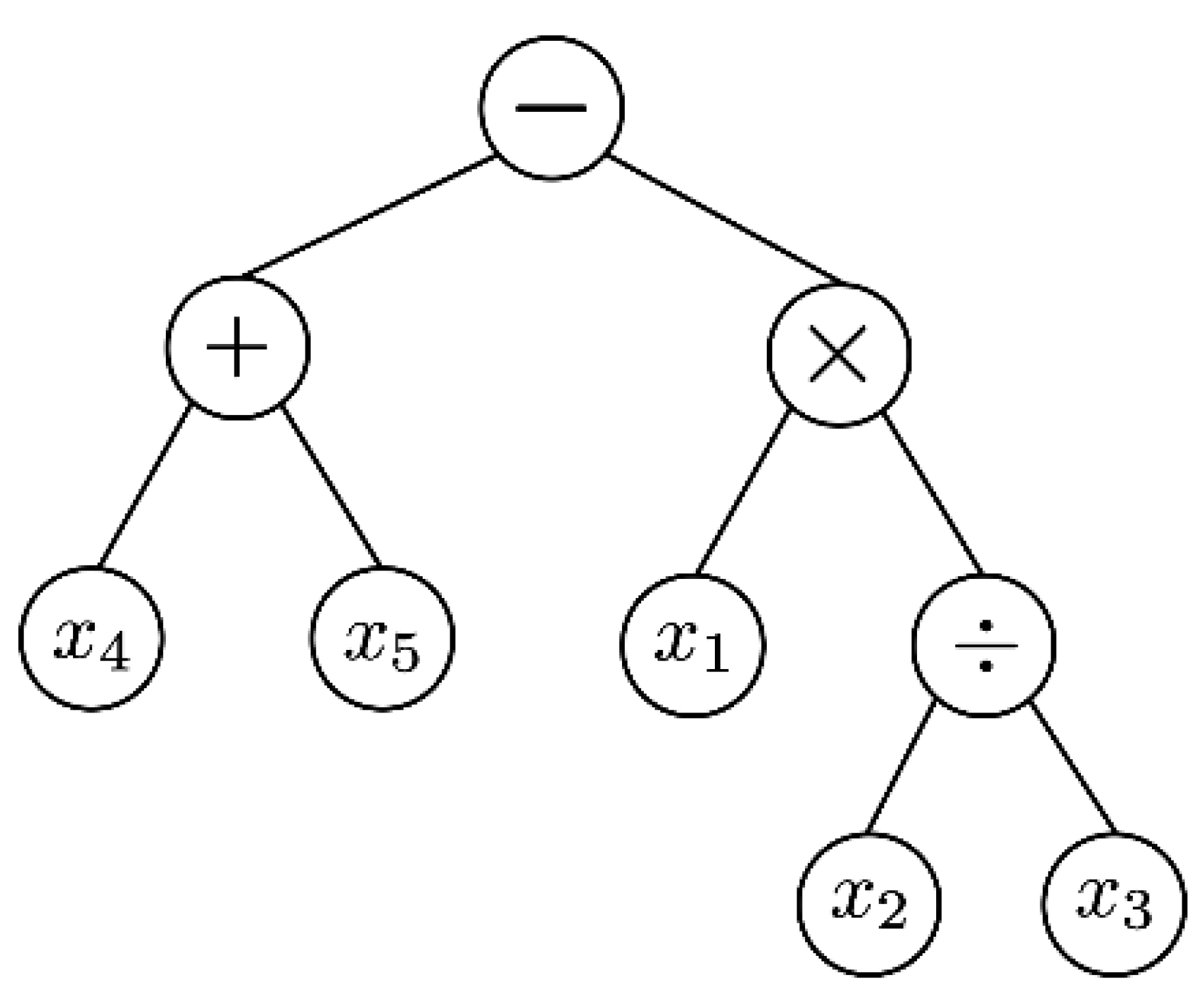
GP is a probabilistic search algorithm which finds an optimal solution through a global search on a population, based on natural selection or survival of the fittest of an ecosystem [15,16]. It is a kind of a stochastic search algorithm. Natural selection or survival of the fittest means that the chromosome of the dominant trait is transferred to the next generation, and the gene of the recessive trait cannot be transferred to the next generation and is left behind. This evolutionary algorithm includes a chromosome encoding, a fitness function, and an operational process that evolves through these stages to obtain a final convergent solution. The genetic operator consists of three operating processes: selection or reproduction, crossover or mating, and mutation. GP used for manufacturing data analysis explains the relationship between input and output variables in a tree structure. By encoding the relationship among input variables using mathematical symbols, it gets more feasible for intuitive interpretation. Here, mathematical operation symbols are assigned to the root node and the middle node of the tree structure, and input variables are assigned to the leaf nodes. Through this method of expressing the solution, it is possible to interpret the result based on the manufacturing principle. This feature makes the analytical result more capable to apply to the real manufacturing field. In Figure 1, the tree expression of the chromosome describes coded mathematical symbols as .
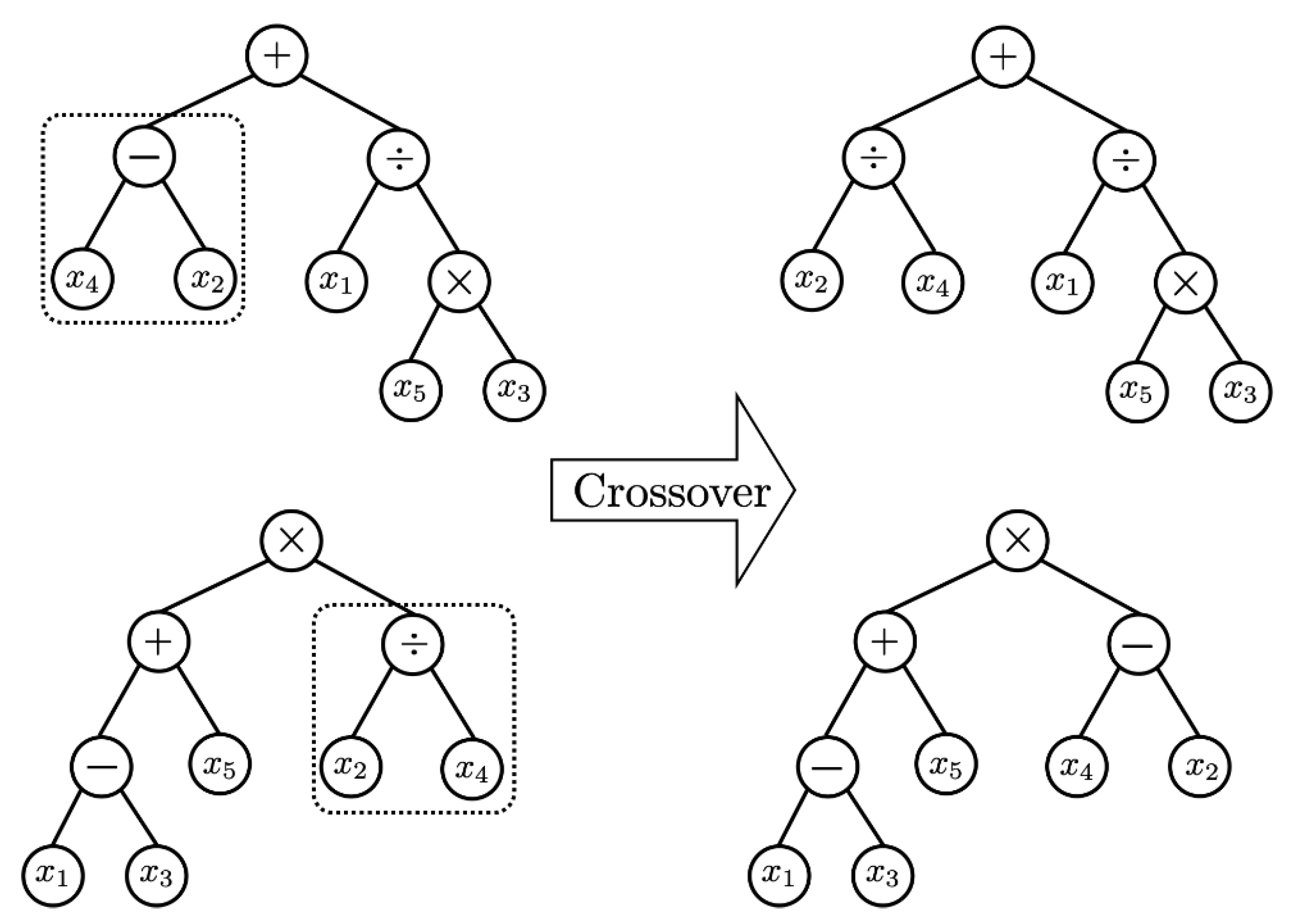
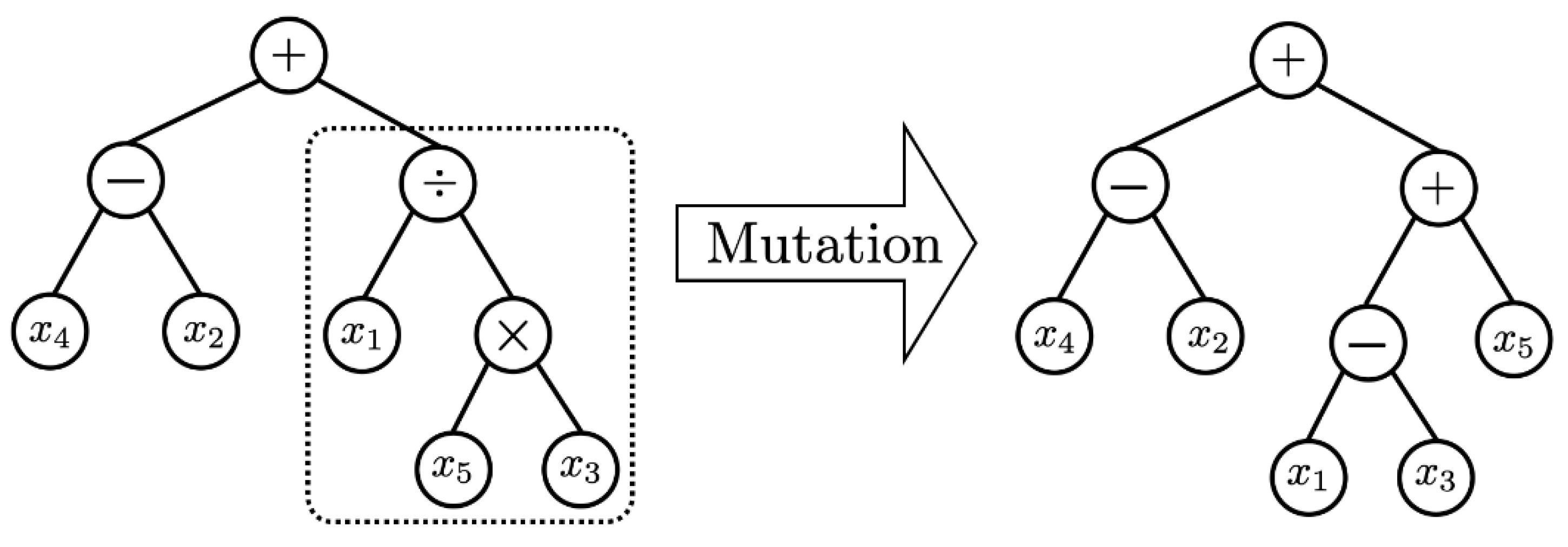
In order to secure the diversity of solutions, genetic operators play an important role. Based on Darwin’s principle of survival of the fittest, the selection or reproduction operators improve the average quality of the population by increasing the likelihood that high-quality chromosomes are passed on to the next generation. The selection technique aims to intensively search the area where the optimal solution exists on the solution-surface. In this paper, many different chromosomes were selected from the population using tournament selection without replacement, and the chromosome with the best fit was selected as the parent chromosome for the next generation. Then, the crossover operator generates offspring chromosomes with superior traits by exchanging partial chromosomes of two parent chromosomes. In other words, the hybridization technique is a method to search the solution-surface of a specific region where the possibility of the existence of an optimal solution is high. In this paper, a hybridization method that does not depend on the location of the gene is used. Regardless of the location of the genes of the two selected chromosomes, a set of locus pairs of genes containing the same node (allele) is formed [15,16]. And the mating operation of the proposed algorithm is illustrated in Figure 2. The last genetic operator, mutation, mutates a gene on a chromosome to another allele to maintain the genetic diversity of the population. The purpose of this operation is to prevent the GP from converging to a quasi-optimal solution, and to search all solution-surfaces for the most optimal solution. However, convergence and optimal performance may be poor when a large number of chromosomes are mutated, because chromosomes may be randomly distributed on the large solution-surface of the population. Mutation creates a modified form of chromosome, which searches the solution-surface of a region that cannot be reached by the existing population. Although the mutation behavior may slightly reduce the convergence performance of GP, it alleviates the possibility of convergence to quasi-optimal solution by preserving the genetic diversity of the population and by creating new partial input variable relationships [15,16]. Figure 3 depicts the process of mutation behavior. Due to these strengths of GP, we are able to discover explainable solutions in big data sets of manufacturing industries. The solution expressed by the tree structure is fairly intuitive for explaining the relationship between input and output variables. As the generation evolves, the length of the tree will be much longer than previous generations, because it generally tends to find solutions with higher accuracy.
In the next section, we propose a manufacturing data analysis technique under a new genetic programming with self-adaption for acquiring more explainable and accurate solutions in high-dimensional manufacturing data. The main operation in our proposed method is to manage the probabilities of crossover and mutation; that is, the length of each solution. Our method overcomes the limitations of previous manufacturing data analysis methods that cannot interpret the analysis results profoundly.
3. Self-Adaptive Genetic Programming (SAGP)
In principle, we propose a predictive analysis method for manufacturing big data using the newly designed self-adaptive genetic programming (SAGP) that follows all GP procedures described in Section 2.2. The main purpose of SAGP is to effectively improve the lack of explanatory power on the result of the analysis algorithm and manufacturing mechanism. In general, black-box-based algorithms are impossible to describe the relationship among the given variables; therefore, they require demanding reinterpretation based on manufacturing principles. In order to deal with these constraints, this paper utilizes GP based predictive modeling method that can formulate the relationship between input and output variables collected during the manufacturing process. However, GP makes the analysis between the features of the data difficult due to the symmetric characteristics. In other words, the tree structured solutions of GP become more complicated to achieve solutions with higher accuracy through evolution stages [17,18,19,20,21,22,23]. In order to achieve symmetrically balanced solutions between high accuracy and high interpretation, this paper applies the self-adaptive technique into GP, named SAGP. It mainly aims to mitigate the complexity of tree expression by managing the probabilities of genetic operators such as crossover and mutation in each generation. It is operated by comparing the previous and current length of tree expressions. First, there is the newly designed probability of crossover defined as
where is the previous average length of solutions and is the current average length of solutions. The maximum probability of crossover is set to 0.75 when the value of is greater than 0.9. As comparing the lengths of previous and present solutions, it is able to achieve better interpretation with a more suitable length of tree expression in the generation. Last, there is the redesigned mutation probability defined as
where is the average length of previous solutions and is the average length of current solutions. The maximum probability of mutation is set to 0.15 if the value of is greater than 0.5. With self-adapted probabilities of crossover and mutation, the proposed method achieved various and superior solutions.
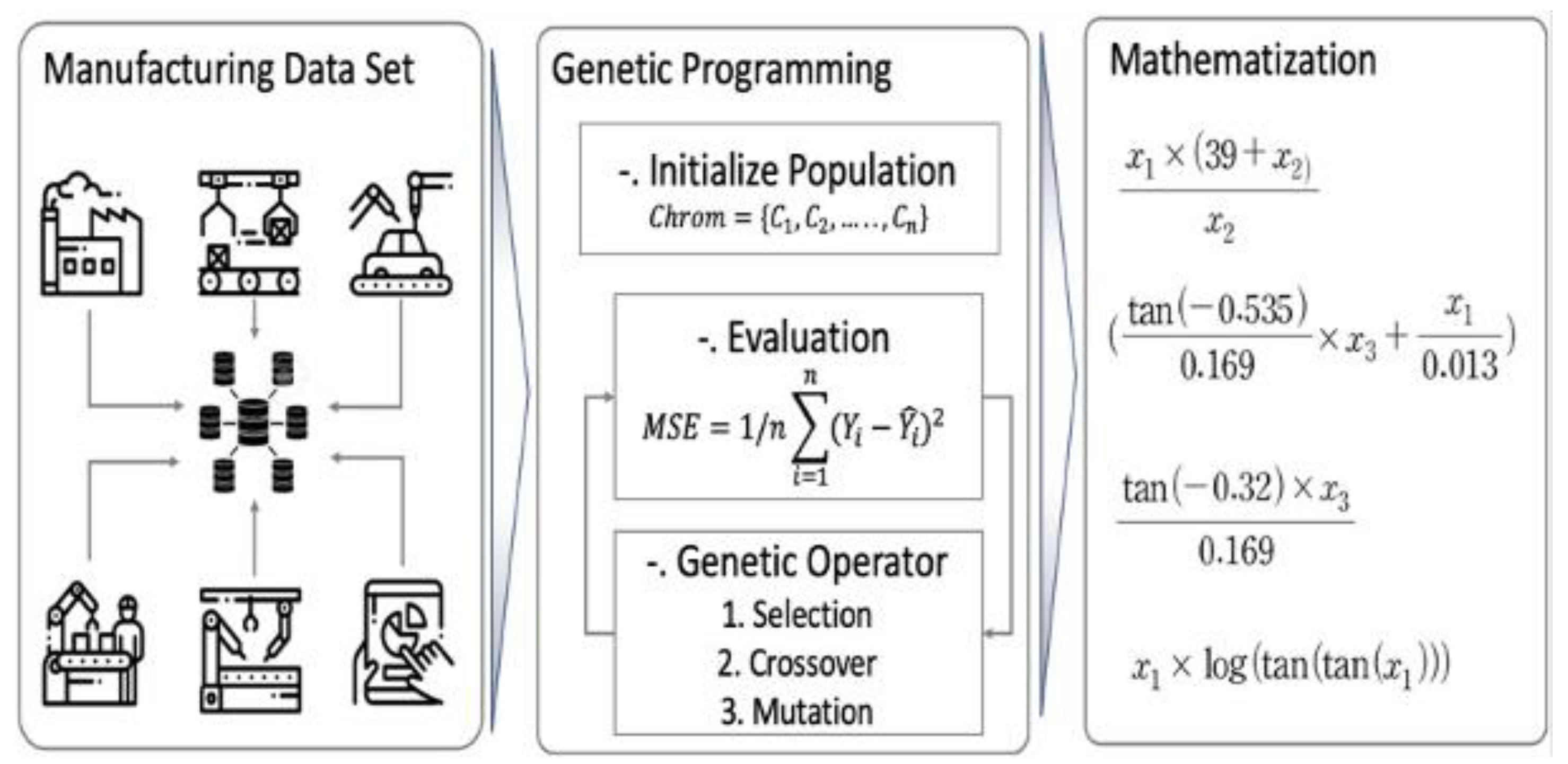
Next, Figure 4 explains the manufacturing big data analysis method employing the proposed algorithm. The big data collected at the manufacturing site is converted into input and output variables through data preprocessing. Then, SAGP algorithm is used to derive a solution representing the relationship of optimal variables by utilizing the tree expression. This can be applied in the actual field through analysis based on manufacturing principles. In addition, it is possible to derive manufacturing principles that could not be interpreted in the past through other analysis methods. In the next section, we compare and verify the performance of machine learning algorithm-based data analysis methods and the proposed SAGP application analysis method using four types of actual manufacturing data.
4. Comparative Results
In this section, we compare and analyze the performance of the proposed self-adaptive genetic programming (SAGP) application analysis method and other representative machine learning algorithm analysis methods using four actual manufacturing data sets. For performance evaluation, the difference between the predicted value and the measured value is estimated using the mean squared error. Also, 80% of the total data is used as training data and the remaining 20% of the total data is used as test data to verify the performance of the analysis methods. In addition, by repeating the experiment 100 times under the same conditions, we intend to secure statistical confidence in the results by utilizing the mean value, standard deviation, and quartile of the repeated experiment. At first, in GP and SAGP, the size of a population and the generation are set to and , respectively. Then, the set of function is defined with . In case of GP, the crossover and mutation are fixed by 0.9 and 0.01. To inspect the performance comparisons, Lasso, Ridge, and Elastic Net algorithm used the optimal normalization method for penalty term control. Support Vector Machine (SVM) used the data normalization of Z-Score (mean = 0 and standard deviation = 1). For Random Forest (RF), the number of variables in each node was set to and the number of trees to create was defined as 500. Neural Network (NN) employed the min-max normalization . In NN, the number of hidden nodes is set to and the maximum iterations are set to , respectively.
The details of the experiment are as follows. We used PC equipped with an Intel(R) Core (TM) i7 6700, 340 Hz CPU and 32 GB RAM. GP and SAGP were experimented with codes written in Python, and the rest of the algorithms were experimented with codes written in R [9]. Meanwhile, the time complexity of GP, one of meta-heuristic algorithms for searching global optimal solution, cannot be determined because it does not guarantee the global optimal solution within a given time limit. However, we carefully speculate that the average-case complexity of SAGP will be lower than the average-case complexity of GP due to adjusting probabilities of genetic operators (i.e., crossover and mutation). Big data analysis, especially in the manufacturing industry, extracts meaningful values from large amounts of structured, or unstructured, data sets. For all data sets used in this study, performance was verified by converting unstructured data into structured data through various data preprocessing processes.
4.1. Auto MPG Data Set Simulation Result
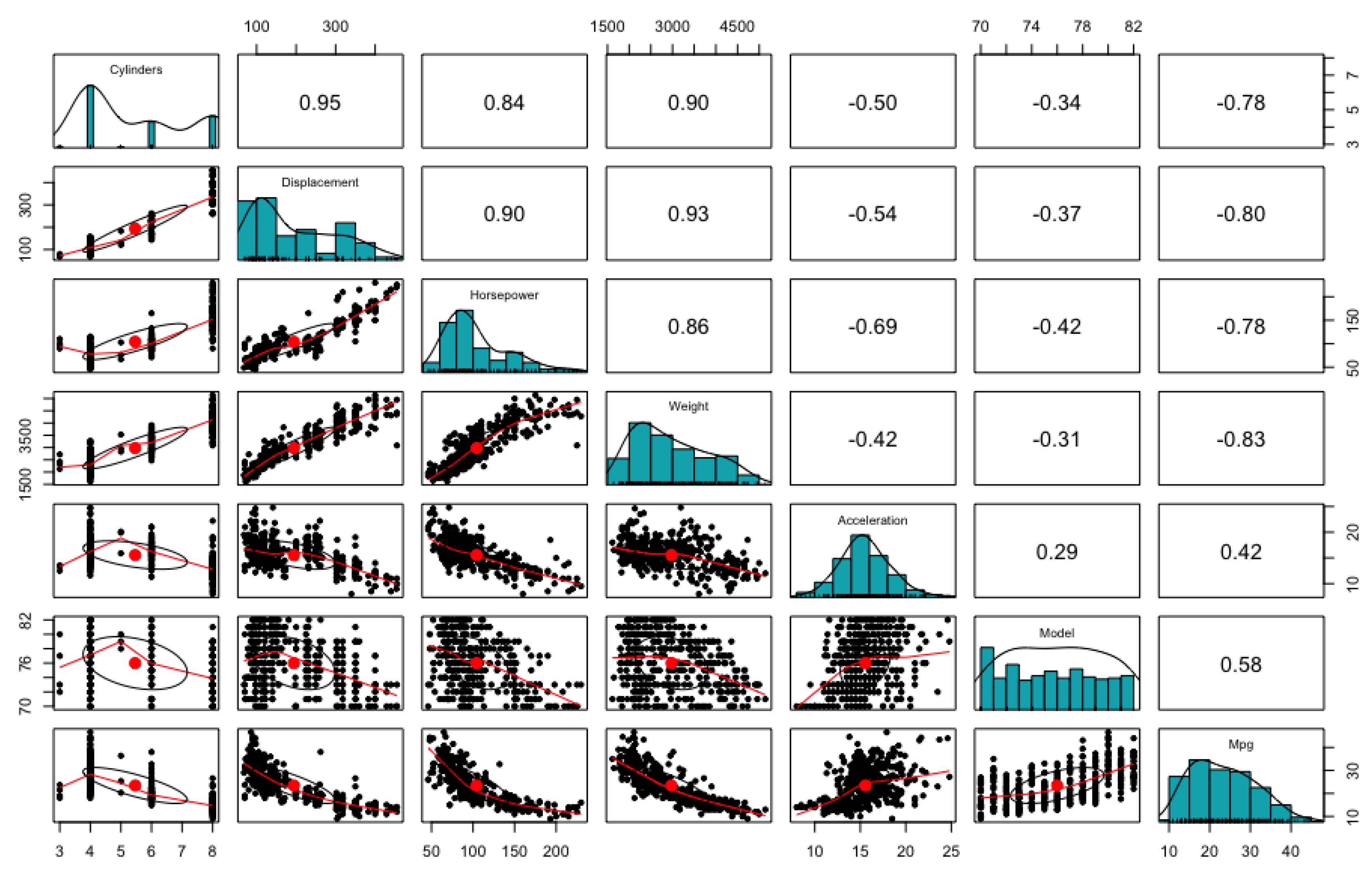
The first dataset we used is the Auto MPG Data, which was first introduced in 1983 by American Statistical Association Exposition. The cycle fuel consumption (mpg cylinder) is used as an output variable with a total of 6 input variables including 3 discrete variables (cylinder, horsepower, model, year) and 3 continuous variables (displacement, weight, acceleration). The given data consists of a total of 398 rows, but the performance is verified using only 391 rows through data preprocessing that eliminates missing data [24,25]. Figure 5 shows the distribution of input and output variables and the degree of correlation between variables. Here, the output variable of mpg, has a positive/negative correlation with all input variables, and the correlation exists among input variables. Table 1 shows that all genetic programming application analysis method and black box-based machine learning techniques (SVM, RF, NN) showed outstanding performance, and the regression analysis algorithms showed low consistency. It is possible to confirm the limitation of the regression analysis technique in real data which has complex relationships among variables. Equations derived from each algorithm are described in Table 2.
4.2. Combined Cycle Plant Data Set Simulation Result
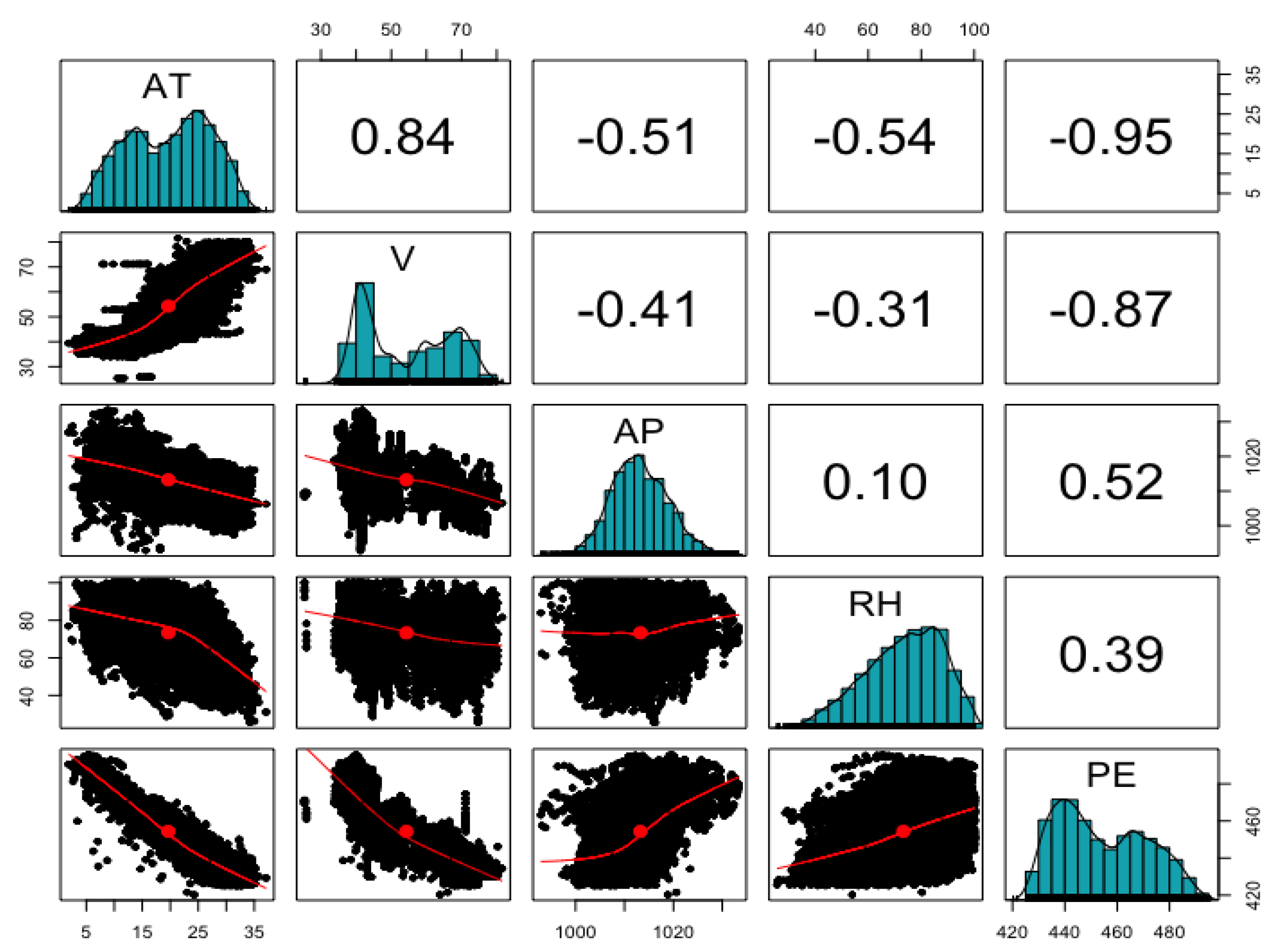
The second data we employed is the Combined Cycle Plant Data consisting of the hourly electrical energy output (PE) of the combined cycle power plant over the period 2006–2011, and the average ambient temperature (AT), ambient pressure (AP), relative humidity (RH), and evacuation vacuum (V) [24,26]. Figure 6 shows the distribution of input and output variables as well as the degree of correlation among variables. Here, the energy output variable has strong negative correlations of −0.95 and −0.87 with average ambient temperature and exhaust vacuum; and positive correlations of 0.52 and 0.39 with ambient pressure and relative humidity. In addition, the time-averaged ambient temperature variable has various positive or negative correlations with the remaining input variables. In Table 3, the black box-based machine learning technique (SVM, RF, NN) showed the best performance compared to the genetic programming-based analysis algorithm, while linear, Lasso, and Elastic net regression methods showed high consistency. Equations derived from each algorithm are described in Table 4.
4.3. CPU Perfoemance Data Set Simulation Result
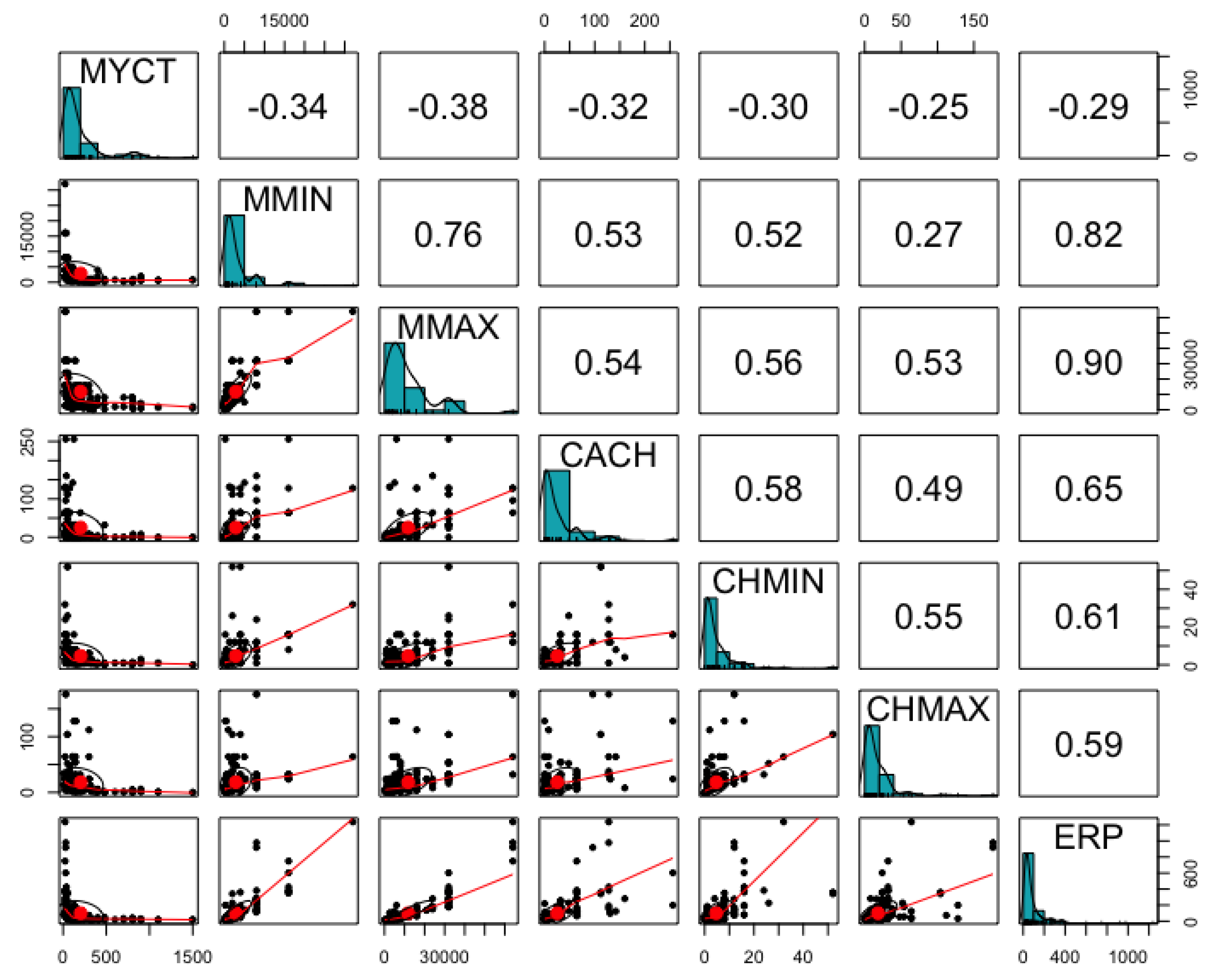
The CPU Performance data consists of total 6 integer input variables including Machine cycle time (MYCT), minimum main memory (MMIN), maximum main memory (MMAX), cache memory (CACH), minimum channels in units (CHMIN), maximum channels in units (CHMAX) in order to predict the dependent variable, estimated relative performance (ERP) [24,27]. Figure 7 shows the distribution of input and output variables, and the mean is skewed to the left in all variables. There is a positive correlation of 0.82, 0.90, 0.65, 0.61, and 0.59 between the predictor variable (ERP) and the input variables MMIN, MMAX, CACH, CHMIN, and CHMAX, respectively. In addition, only the MYCT variable has a negative correlation with all other variables, whereas all other variables have a positive correlation reciprocally. Table 5 shows the results of comparing the data-based performance. The genetic programming-based analysis showed the best performance, and the black-box-based machine learning technique, Random Forest, showed the second-best performance. Regression analysis showed significant performance, but SVM showed the lowest consistency. In the case of integer data, SVM may have limit in securing consistency. Among representative machine learning techniques on actual manufacturing data, the difference in performance occurs according to the complexity of the data. In general, the black-box-based machine learning technique, Random Forest, showed excellent performance. However, since the analysis result lacks explanatory power for derivation, an additional manufacturing process-based analysis process is required in order to apply to the actual manufacturing field. In addition, for data with a linear relationship, the regression analysis technique showed outstanding performance, but the analysis results are derived with linear equations that the explanatory power is monotonous. However, linear equations show significant consistency with respect to the linear or nonlinear analysis results. Equations derived from each algorithm are described in Table 6.
4.4. Real Manufacuring Process Data Set Simulation Result
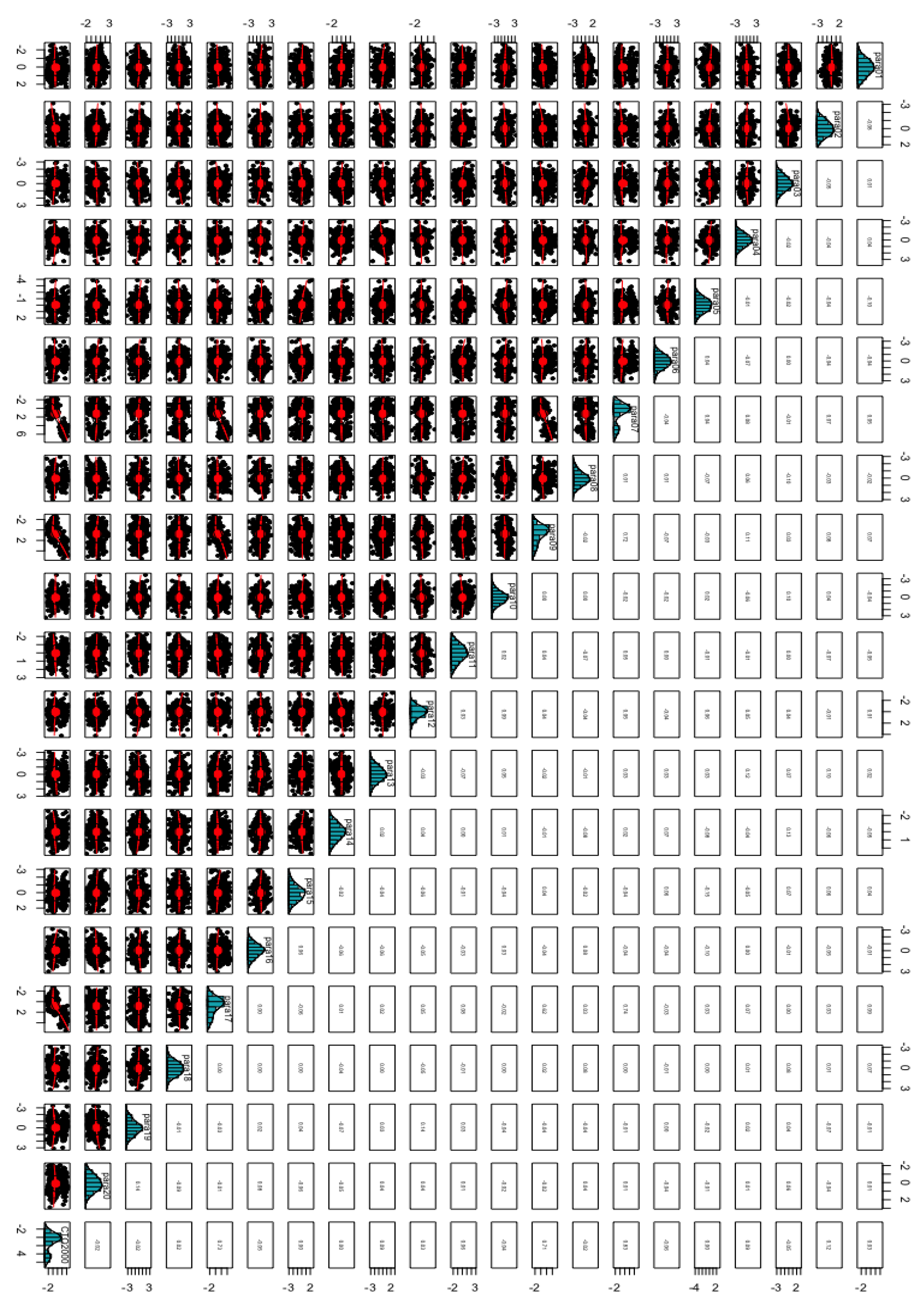
In general, data collected and utilized in the manufacturing process is composed of multidimensional input data. However, it is difficult to intuitively analyze the relationship between various factors. To solve this problem, a preliminary analysis is performed on collected data based on the domain knowledge of the manufacturing process, but it is still almost impossible to analyze the relationship between factors. Also, classification and prediction analysis were not so different that the results were barely available for interpretation on the relationship between factors. The main difficulty is that it is implausible to derive an accurate result through classification or prediction based on the performed analysis. This section attempts to verify the performance of the algorithm by using 20 process factors and quality result data collected from a specific manufacturing company. Detailed explanations on the data, however, are excluded due to security issues in the manufacturing process of the company that provided the data. (see Figure 8)
The performance of each company was verified for a total of 20 process factors affecting the main quality factors. In Table 7, our proposed technique shows superior performance compared to regression analysis methods and SVM, while it showed poor performance compared to RF. Here, in the case of RF, there is a disadvantage that it is impossible to interpret the results derived by the black-box-based machine learning algorithm. However, in the case of our proposed algorithm, it is possible to analyze the relationship between the key quality factors and 20 process factors. It can classify factors that have high influence and analyze the relationship among factors. The equations derived from each algorithm are described in Table 8.
5. Conclusions
In this study, we propose a genetic programming-based analysis method to overcome the limitations of the black-box-based machine learning algorithms. Existing machine learning algorithms have high predictive consistency, but especially in the manufacturing industry, it is important to verify the basis of the results and the validity of derivation through analysis based on the manufacturing process principle. In the case of our proposed analysis method, intuitive analysis based on manufacturing principles is plausible through formulating the relationship of input and output variables. It is also possible to derive manufacturing principles that could not be interpreted in the past, by using the analysis result which formulates the input and output variables. As a result, SAGP showed excellent performance on manufacturing data compared to other analysis methods and machine learning algorithms. Nevertheless, our proposed method did not search for the optimal tree depth according to the problem size. Further studies on finding the optimal tree depth will enhance the performance of our proposed method, as the length of tree depth seriously affects the symmetry between interpretation and accuracy of tree expression. In the future, we plan to conduct further research on improving the explanatory power and analytical consistency for manufacturing big data analysis.
Author Contributions
Conceptualization, S.O. and C.-W.A.; methodology, S.O. and C.-W.A.; software, S.O. and W.-H.S.; investigation, C.-W.A.; data curation, S.O.; writing—original draft preparation, S.O. and W.-H.S.; writing—review and editing, C.-W.A.; visualization, S.O. and W.-H.S.; supervision, C.-W.A.; funding acquisition, C.-W.A. All authors have read and agreed to the published version of the manuscript.
Funding
This work was supported by IITP grant funded by the Korea government (MSIT) (No. 2019-0-01842, Artificial Intelligence Gradate School Program (GIST)), and the National Research Foundation of Korea (NRF) funded by the Ministry of Education (NRF-2021R1A2C3013687).
Conflicts of Interest
The authors declare no conflict of interest.
References
- Game Changers: Five Opportunities for US Growth and Renewal. Available online: https://www.mckinsey.com/featured-insights/americas/us-game-changers (accessed on 1 July 2013).
- Data Economy in the Energy Landscape—V. Available online: https://www.eitdigital.eu/newsroom/blog/article/data-economy-in-the-energy-landscape-v/ (accessed on 6 August 2015).
- Big Data Is the Future of Industry, Says GE. Available online: https://www.information-age.com/big-data-is-the-future-of-industry-says-ge-123457136/ (accessed on 19 June 2013).
- Intel Cuts Manufacturing Costs with Big Data. Available online: https://www.informationweek.com/software/information-management/intel-cuts-manufacturing-costs-with-big-data/d/d-id/1109111 (accessed on 18 March 2013).
- Arun, K.; Jabasheela, L. Big Data: Review, Classification and Analysis Survey. Int. J. Innov. Res. Inf. Secur. 2014, 1, 17–23. [Google Scholar]
- Principal Component Regression. Available online: https://en.wikipedia.org/wiki/Principal_component_regression (accessed on 24 December 2020).
- Duda, R.O.; Hart, P.E.; Stork, D.G. Pattern Classification, 2nd ed.; Wiley-Interscience: Hoboken, NJ, USA, 2012. [Google Scholar]
- Breiman, L. Random Forests. Mach. Learn. 2015, 45, 5–32. [Google Scholar] [CrossRef] [Green Version]
- Lantz, B. Machine Learning with R, 2nd ed.; Packt: Birmingham, UK, 2015. [Google Scholar]
- Hashmi, A.S.; Ahmad, T. Big Data Mining: Tools & Algorithms. Int. J. Recent Contrib. Eng. 2016, 4, 36. [Google Scholar] [CrossRef] [Green Version]
- Witten, I.H.; Eibe, F. Data Mining: Practical Machine Learning Tools and Techniques; Morgan Kaufmann Publishers: San Francisco, CA, USA, 2005. [Google Scholar]
- Bishop, C.M. Pattern Recognition and Machine Learning; Springer Science & Media: New York, NY, USA, 2009. [Google Scholar]
- Mittchel, T. Machine Learning; Computer Science Series; McGRAW HILL International: New York, NY, USA, 1997. [Google Scholar]
- Oh, S.; Yaochu, J. Incremental Approximation Models for Constrained Evolutionary Optimization. In Evolutionary Constrained Optimization, 1st ed.; Datta, R., Deb, K., Eds.; Springer: New Delhi, India, 2015. [Google Scholar]
- Langdon, W.B. Genetic Programming + Data Structures = Automatic Programming; The Kluwer International Series in Engineering and Computer Science; Kluwer Academic Publishers: Berlin, Germany, 1998. [Google Scholar]
- Banzhaf, W.; Nordin, P.; Keller, R.E.; Francone, F.D. Genetic Programming: An Introduction on the Automatic Evolution of Computer Programs and Its Applications; Morgan Kaufmann Publishers, Inc.: San Francisco, CA, USA, 1997. [Google Scholar]
- Saravanana, N.; Fogel, D.B.; Nelson, K.M. A comparison of methods for self-adaptation in evolutionary algorithms. Biosystems 1995, 36, 157–166. [Google Scholar] [CrossRef]
- Venugopal, K.R.; Srinivasa, K.G.; Patnaik, L.M. Self Adaptive Genetic Algorithms. In Soft Computing for Data Mining Applications; Springer: Berlin/Heidelberg, Germany, 2009; pp. 19–50. [Google Scholar]
- Huang, L.; Ding, L.; Du, W. Improved Self-Adaptive Genetic Algorithm with Varying Population Size. In Proceedings of the 2009 Fifth International Conference on MEMS NANO, and Smart Systems, Dubai, United Arab Emirates, 28–30 December 2009; pp. 77–79. [Google Scholar]
- Dulebenets, M.A.; Kavoosi, M.; Abioye, O.; Pasha, J. A Self-Adaptive Evolutionary Algorithm for the Berth Scheduling Problem: Towards Efficient Parameter Control. Algorithms 2018, 11, 100. [Google Scholar] [CrossRef] [Green Version]
- Beasley, D.; Bull, D.R.; Martin, R.R. An Overview of Genetic Algorithms: Part 1, Fundamentals. Univ. Comput. 1993, 15, 58–69. [Google Scholar]
- Chang Wook, A. Advances in Evolutionary Algorithms: Theory, Design and Practice; Springer: Berlin/Heidelberg, Germany, 2006. [Google Scholar]
- Whigham, P.A. Inductive bias and genetic programming. In Proceedings of the First International Conference on Genetic Algorithms in Engineering Systems: Innovations and Applications, Sheffield, UK, 12–14 September 1995; pp. 461–466. [Google Scholar]
- Auto-mpg Dataset (Mileage Per Gallon Performances of Various Cars). Available online: https://www.kaggle.com/uciml/autompg-dataset (accessed on 2 July 2017).
- Combined Cycle Powerplant. Available online: https://www.kaggle.com/gova26/airpressure (accessed on 27 August 2019).
- Relative CPU Performance Data. Available online: https://www.kaggle.com/balajisriraj/relative-cpu-performance-data (accessed on 23 November 2018).
- Dua, D.; Graff, C. UCI Machine Learning Repository 2019. Available online: http://archive.ics.uci.edu/ml (accessed on 16 April 2021).
Figure 1.
Tree Expression of GP.

Figure 2.
Example of Crossover in GP.

Figure 3.
Example of Mutation in GP.

Figure 4.
SAGP based manufacturing big data analysis.

Figure 5.
Scatterplot Matrix of Auto MPG Data Set.

Figure 6.
Scatterplot Matrix of Cycle Plant Data Set.

Figure 7.
Scatterplot Matrix of CPU Performance Data Set.

Figure 8.
Scatterplot Matrix of Real Manufacturing Process Data Set.


Table 1.
Simulation Result of Auto MPG Data Set.
| LR | Lasso | Ridge | Elastic | PLS | SVM | RF | NN | GP | SAGP | |
|---|---|---|---|---|---|---|---|---|---|---|
| Mean | 13.28 | 13.24 | 13.79 | 13.28 | 18.9 | 8.32 | 8.23 | 12.40 | 7.48 | 6.83 |
| Std | 1.32 | 1.35 | 1.48 | 1.37 | 1.85 | 1.3 | 1.19 | 2.82 | 1.3 | 1.54 |
| Q0 | 9.33 | 9.16 | 9.39 | 9.2 | 14.51 | 5.73 | 6.14 | 7.16 | 4.94 | 4.8 |
| Q1 | 11.47 | 11.46 | 11.83 | 11.53 | 18.06 | 7.47 | 7.69 | 10.28 | 6.06 | 6.24 |
| Q2 | 12.17 | 12.02 | 12.51 | 12.06 | 19.04 | 8.3 | 8.39 | 11.97 | 6.84 | 6.83 |
| Q3 | 13.13 | 13.19 | 13.69 | 13.15 | 20.27 | 9.34 | 9.33 | 14.26 | 7.45 | 7.77 |
| Q4 | 17.48 | 17.38 | 17.26 | 17.32 | 25.85 | 12.3 | 12.14 | 19.68 | 11.92 | 14.86 |
| 95% CI (Lower) | 13.02 | 12.98 | 13.5 | 13.02 | 18.54 | 8.06 | 8.00 | 11.84 | 7.22 | 6.53 |
| 95% CI (Upper) | 13.54 | 13.51 | 14.08 | 13.55 | 19.26 | 8.58 | 8.46 | 12.95 | 7.73 | 7.13 |
| 95% CI | 0.52 | 0.53 | 0.58 | 0.53 | 0.72 | 0.51 | 0.46 | 1.11 | 0.51 | 0.60 |
Table 2.
Example of Performance Results.
| LR | |
| Lasso | |
| Ridge | |
| Elastic | |
| GP | |
| SAGP |
Table 3.
Simulation Result of Cycle Plant Data Set.
| LR | Lasso | Ridge | Elastic | PLS | SVM | RF | NN | GP | SAGP | |
|---|---|---|---|---|---|---|---|---|---|---|
| Mean | 22.36 | 22.32 | 24.82 | 22.32 | 60.3 | 17.53 | 13.22 | 17.02 | 35.16 | 29.31 |
| Std | 0.49 | 0.48 | 0.55 | 0.48 | 1.42 | 0.49 | 0.45 | 0.28 | 3.09 | 3.05 |
| Q0 | 19.76 | 19.77 | 23.03 | 19.78 | 55.98 | 15.08 | 11.02 | 16.36 | 25.79 | 28.17 |
| Q1 | 20.58 | 20.58 | 23.64 | 20.57 | 59.49 | 16.00 | 11.77 | 16.84 | 31.39 | 32.24 |
| Q2 | 20.85 | 20.86 | 24.02 | 20.87 | 60.17 | 16.33 | 12.09 | 17.01 | 33.75 | 33.94 |
| Q3 | 21.27 | 21.27 | 24.42 | 21.29 | 61.07 | 16.64 | 12.4 | 17.18 | 35.71 | 35.50 |
| Q4 | 22.36 | 22.32 | 25.54 | 22.32 | 64.03 | 17.53 | 13.22 | 17.79 | 40.91 | 41.75 |
| 95% CI (Lower) | 22.26 | 22.23 | 24.72 | 22.22 | 60.02 | 17.43 | 13.14 | 16.96 | 34.55 | 28.71 |
| 95% CI (Upper) | 22.45 | 22.42 | 24.93 | 22.41 | 60.58 | 17.62 | 13.31 | 17.07 | 35.76 | 29.91 |
| 95% CI | 0.19 | 0.19 | 0.21 | 0.19 | 0.56 | 0.19 | 0.17 | 0.11 | 1.21 | 1.20 |
Table 4.
Example of Performance Results.
| LR | |
| Lasso | |
| Ridge | |
| Elastic | |
| GP | |
| SAGP |
Table 5.
Simulation Result of CPU Performance Data Set.
| LR | Lasso | Ridge | Elastic | PLS | SVM | RF | NN | GP | SAGP | |
|---|---|---|---|---|---|---|---|---|---|---|
| Mean | 8917.41 | 8781.47 | 8581.84 | 8766.61 | 6360.73 | 13,783.18 | 7424.47 | 30,523.62 | 2629.84 | 1637.18 |
| Std | 2822.74 | 2779.28 | 2741.89 | 2787.66 | 2413.88 | 8311.6 | 4717.28 | 11,305.88 | 1677.42 | 1583.52 |
| Q0 | 1811.6 | 1752.54 | 1645.4 | 1720.66 | 2928.26 | 1227.97 | 638.22 | 1024.10 | 892.00 | 892.00 |
| Q1 | 4147.05 | 4206.36 | 3932.02 | 4124.51 | 5563.24 | 5002.22 | 1576.33 | 21,434.54 | 1902.12 | 2086.18 |
| Q2 | 5376.54 | 5522.51 | 5306.33 | 5489.76 | 6523.14 | 10,947.52 | 3444.87 | 31,349.62 | 2746.01 | 2545.12 |
| Q3 | 6855.99 | 6785.07 | 6905.27 | 6736.14 | 7788.72 | 17,058.42 | 6815.02 | 36,768.88 | 4024.56 | 3976.83 |
| Q4 | 14,367.02 | 14,390.59 | 14,853.25 | 14,967.82 | 15,519.83 | 36,188.42 | 20,530.4 | 54,896.24 | 8326.26 | 8785.96 |
| 95% CI (Lower) | 8364.15 | 8236.73 | 8044.43 | 8220.23 | 5887.61 | 12,154.11 | 6499.89 | 28,307.66 | 2301.06 | 1326.81 |
| 95% CI (Upper) | 9470.67 | 9326.21 | 9119.25 | 9319.99 | 6833.85 | 15,412.26 | 8349.06 | 32,739.57 | 2958.61 | 1947.55 |
| 95% CI | 1106.52 | 1089.48 | 1074.82 | 1099.76 | 946.24 | 3258.15 | 1849.17 | 4431.91 | 657.55 | 620.74 |
Table 6.
Example of Performance Results.
| LR | |
| Lasso | |
| Ridge | |
| Elastic | |
| GP | |
| SAGP |
Table 7.
Simulation Result of Real Manufacturing Process Data Set.
| LR | Lasso | Ridge | Elastic | PLS | SVM | RF | NN | GP | SAGP | |
|---|---|---|---|---|---|---|---|---|---|---|
| Mean | 1.29 | 1.21 | 1.31 | 1.22 | 1.17 | 1.53 | 1.02 | 3.92 | 1.82 | 1.18 |
| Std | 0.12 | 0.12 | 0.12 | 0.12 | 0.11 | 0.14 | 0.09 | 0.80 | 0.26 | 0.26 |
| Q0 | 1.08 | 1.06 | 1.14 | 1.04 | 1.07 | 1.37 | 0.83 | 2.59 | 1.06 | 1.08 |
| Q1 | 1.40 | 1.36 | 1.43 | 1.37 | 1.31 | 1.60 | 0.98 | 3.34 | 1.43 | 1.44 |
| Q2 | 1.49 | 1.43 | 1.49 | 1.44 | 1.36 | 1.71 | 1.03 | 3.91 | 1.58 | 1.60 |
| Q3 | 1.55 | 1.51 | 1.57 | 1.51 | 1.45 | 1.80 | 1.09 | 4.33 | 1.76 | 1.77 |
| Q4 | 1.89 | 1.77 | 1.83 | 1.82 | 1.69 | 2.07 | 1.24 | 6.23 | 2.39 | 2.33 |
| 95% CI (Lower) | 1.27 | 1.19 | 1.29 | 1.19 | 1.15 | 1.50 | 1.01 | 3.76 | 1.77 | 1.13 |
| 95% CI (Upper) | 1.31 | 1.24 | 1.34 | 1.24 | 1.2 | 1.56 | 1.04 | 4.07 | 1.87 | 1.23 |
| 95% CI | 0.04 | 0.05 | 0.05 | 0.05 | 0.05 | 0.06 | 0.03 | 0.31 | 0.10 | 0.10 |
Table 8.
Example of Performance Results.
| LR | |
| Lasso | |
| Ridge | CTQ = 0.148 + 0.056 × Para1 + 0.0722 × Para2 − 0.080 × Para3 + 0.033 × Para4 − 0.153 × Para5 − 0.024 × Para6 + 0.425 × Para7 − 0.118 × Para8 + 0.291 × Para9 − 0.151 × Para10 − 0.47 × Para12 + 0.187 × Para13 − 0.004 × Para14 − 0.051 × Para15 − 0.090 × Para16 + 0.330 × Para17 + 0.098 × Para18 + 0.044 × Para19 − 0.049 × Para20 |
| Elastic | CTQ = 0.139 + 0.028 × Para2 − 0.029 × Para3 − 0.105 × Para5 + 0.469 × Para7 − 0.054 × Para8 + 0.272 × Para9 − 0.116 × Para10 + 0.147 × Para13 − 0.032 × Para16 + 0.286 × Para17 + 0.047 × Para18 |
| GP | |
| SAGP |
Publisher’s Note: MDPI stays neutral with regard to jurisdictional claims in published maps and institutional affiliations. |
© 2021 by the authors. Licensee MDPI, Basel, Switzerland. This article is an open access article distributed under the terms and conditions of the Creative Commons Attribution (CC BY) license (https://creativecommons.org/licenses/by/4.0/).
Share and Cite
MDPI and ACS Style
Oh, S.; Suh, W.-H.; Ahn, C.-W. Self-Adaptive Genetic Programming for Manufacturing Big Data Analysis. Symmetry 2021, 13, 709. https://doi.org/10.3390/sym13040709
AMA Style
Oh S, Suh W-H, Ahn C-W. Self-Adaptive Genetic Programming for Manufacturing Big Data Analysis. Symmetry. 2021; 13(4):709. https://doi.org/10.3390/sym13040709
Chicago/Turabian StyleOh, Sanghoun, Woong-Hyun Suh, and Chang-Wook Ahn. 2021. "Self-Adaptive Genetic Programming for Manufacturing Big Data Analysis" Symmetry 13, no. 4: 709. https://doi.org/10.3390/sym13040709
Note that from the first issue of 2016, this journal uses article numbers instead of page numbers. See further details here.