1. Introduction
Closed Plant Production Systems (CPPS) consist of a wide variety of growing methods, like vertical farms, plant factories, greenhouses, growth chambers, tissue culture rooms, phytotrons, and high tunnels, among others [
1,
2,
3,
4,
5,
6,
7,
8,
9]. The controlled agricultural environments approach allows producers to establish ideal conditions for given crops (e.g., in terms of the quantity and quality of light, humidity, temperature, carbon dioxide, among others). Such an approach yields higher crop production and quality, and means that any variety of plant can be planted at any time of the year. The literature has shown that light-emitting diodes (LEDs) are an energy efficient substitute for other types of lamps (filament lamps and gas discharge lamps with mercury and sodium), and enhance plant growth. The use of LEDs for plant production has transformed the horticultural industry. The radiation emitted by LEDs has various advantages like rapid response time, longer lifetime, controllability, efficiency wavelengths that drive specific responses in plants such as photomorphogenic, biochemical or physiological development, and even the control of pests and diseases. LEDs are programmed to produce continuous irradiation and can also be easily configured to emit rapid (µs) pulsed irradiation (on/off) with heightened intensity and modest energy consumption [
3,
10,
11,
12,
13,
14]. Artificial lighting is a key factor in CPPS and a significant LED technology attribute is the emission of different wavelengths, called light recipes. Light recipes may influence the development and growth of crops from sprouting to flowering, stimulate stem elongation, optimize edible biomass, and increase nutritional content, antioxidant capacity, levels of calcium, potassium, magnesium, and phosphorus, number of fruits, among others [
15,
16,
17]. The mixture of wavelengths (red, blue, green, ultraviolet, and infrared) and the photosynthetic photon flux density (PPFD, or intensity levels given in µmol m
−2 s
−1) are the main components of light recipes. Light recipes are commonly configured in continuous mode, but can also be configured in pulsed mode to save energy. Reducing the energy costs of illumination systems in CPPS, and the fabrication of efficient light devices, are challenges for the near future [
18].
The cost of electricity to supply electrical power to CPPS and greenhouses is high. The cost of the LED lighting system represents 30% of the initial capital cost for a CPPS, while electricity represents 60% of the annual operating costs [
19]. The main part of this electricity is required to generate lighting for crops and air conditioning which is necessary to remove the heat produced by the lighting system [
14]. As such, 40% to 50% of the total operating costs of CPPS are linked to the lighting system [
19,
20]. More efficient lighting strategies are essential to improve the sustainability and profitability of closed plant production systems.
Various research groups have tried to devise innovative approaches to reduce the energy requirements of CPPS. An approach employing energy informatics (energy prices, forecasts of solar radiation, plant specifications and production process) for controlled environment agriculture (CAE) that helps to analyze, design, and implement strategies for a global diagnosis would make it possible to optimize the usage of resources, while also monitoring the lighting systems in the greenhouse. Producers would be informed about energy consumption levels to avoid wasting resources [
21]. Hwang et al. [
22] executed a computational fluid dynamics (CFD) simulation using information collected by sensors connected to the Internet of Things. This study used temperature data and emitted airflow to achieve energy efficiency in plant factories. DynaGrow uses a multiobjective evolutionary algorithm (MOEA) that monitors and detects critical points at which the climate in a greenhouse integrates local climate data, electricity energy price forecasts, and outdoor weather forecasts. Dynagrow showed that it was feasible to grow different plants and improve the use of resources without affecting the quality of the produce [
23]. A mathematical expression to control the temperature in greenhouses based on the fuzzy proportional, integral, and derivative (PID) and the greenhouse temperature model was designed. The graphs obtained through simulations indicated that the model had a short response time and could maintain a stable temperature inside the closed production plant system [
24,
25,
26]. Also, neural networks have been used in CPPS to estimate indoor temperature and humidity [
27], predict climatic conditions [
28,
29] or forecast energy consumption [
30]. Energy prediction models (EPM) to evaluate the energy requirements and performance of the system for the production of plants in closed spaces have been implemented. Similarly, a predictive control model (MPC) has been proposed for temperature regulation through ventilation and optimization of crop production [
31,
32]. Another proposal was a MPC to increase the precision of actuator control and to minimize energy consumption [
33]; the cost of energy, ventilation, and the price of managing CO
2 were the inputs. The aim was the optimization of the greenhouse process, as well as reducing the disturbance and inadaptability of the system [
34].
According to the literature, there are different proposals to monitor, control and predict aspects such as weather conditions, energy consumption, humidity, temperature, and CO
2 levels, among others, in a CPPS. Implemented approaches include computer systems, fluid dynamics, multi-objective evolutionary algorithms (MOEA), Neural Networks, and the predictive control model. However, predictions of energy consumption in artificial lighting systems based on light recipes considering the light operation modes (pulsed and continuous) have not been reported. Hence, it is essential to assume that a challenge for CPPS is to apply strategies to improve energy consumption without affecting crop yield and quality. Aiming to generate new alternatives that may contribute to forecasting CPPS energy consumption, we propose two nonlinear models based on artificial intelligence that support modeling of the energy requirements of the LED lighting. The models include a vector with seven inputs and an output represented by the energy consumption of the CPPS. In the literature, no proposal has yet considered the components of light (red, blue, green, and white) and its mode of operation, i.e., continuous or pulsed (i.e., intensity, pulse frequency, and duty cycle). The first model uses genetic programming (GP), and the second feedforward neural networks (FNNs). We applied and compared these techniques in the generation of nonlinear models because they have been used for this propose [
35,
36,
37,
38,
39,
40,
41]. This research applies 10-fold cross-validation to select the training complexity parameters because this approach almost eliminates the bias of the estimated error [
42,
43,
44,
45,
46]. Ten-fold cross-validation is the most widely used in the literature because, even with random sampling, it reflects the behavior in the original dataset. Furthermore, it has been shown that any increase in the number of folds beyond 10 only increases computational effort, while slightly reducing the variance in the results owing to the number of folds does not impact the dataset distributions [
42,
44,
46].
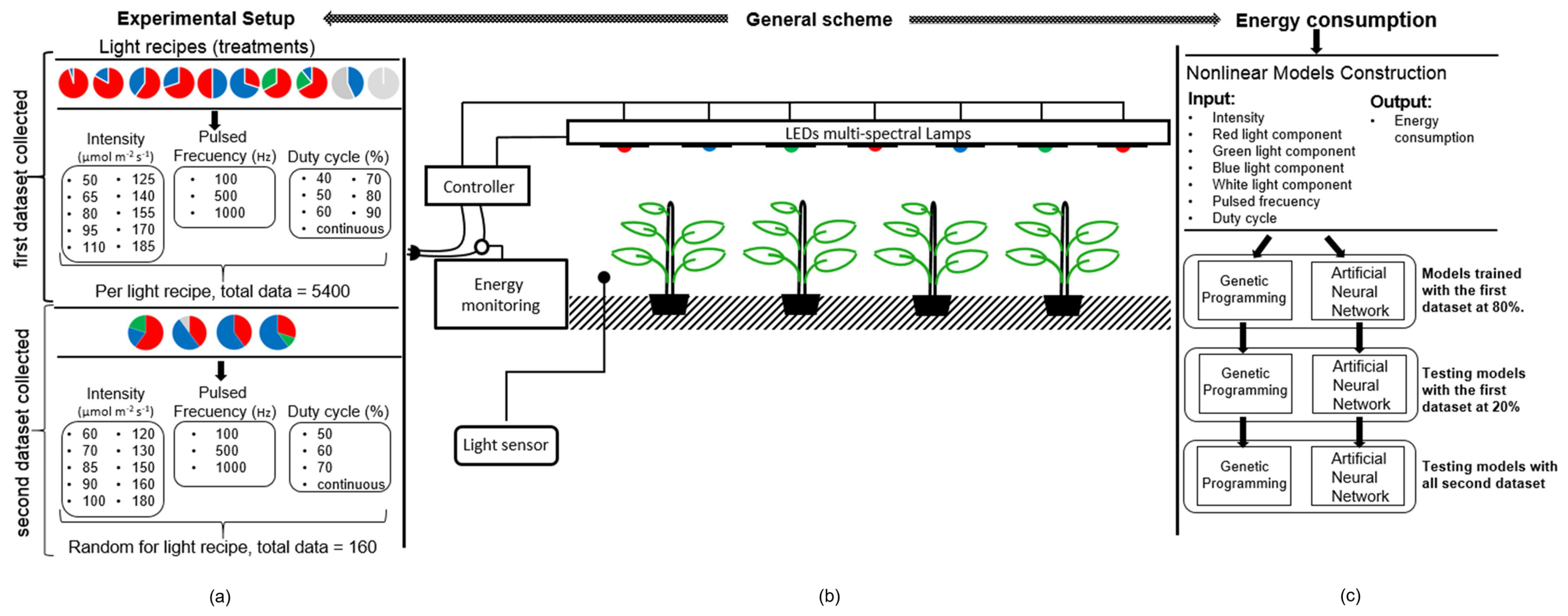
Additionally, we used test values outside the ranges established in the training stage to verify the generalization of the model. A Spearman’s correlation was applied to generate the model only with representative inputs. Different light recipes extracted from the literature that are normally used for plant growth were configured in the artificial lighting system to generate the two datasets. The first (Test 1), with 5700 samples with similar input ranges, was used to train and evaluate, while the second (Test 2) had a total of 160 datapoints from different input ranges. The metrics that allowed a quantitative and statistic evaluation of the model’s performance were mean absolute percentage error (MAPE), mean square error (MSE), mean absolute error (MAE), standard error of the estimate (SEE), the determination coefficient (R2), and One-Way Analysis of Variance (ANOVA). The GP and FNNs models generated in this proposal can be applied or programmed as part of a monitoring system for CPPS which prioritize energy efficiency.
3. Results and Discussion
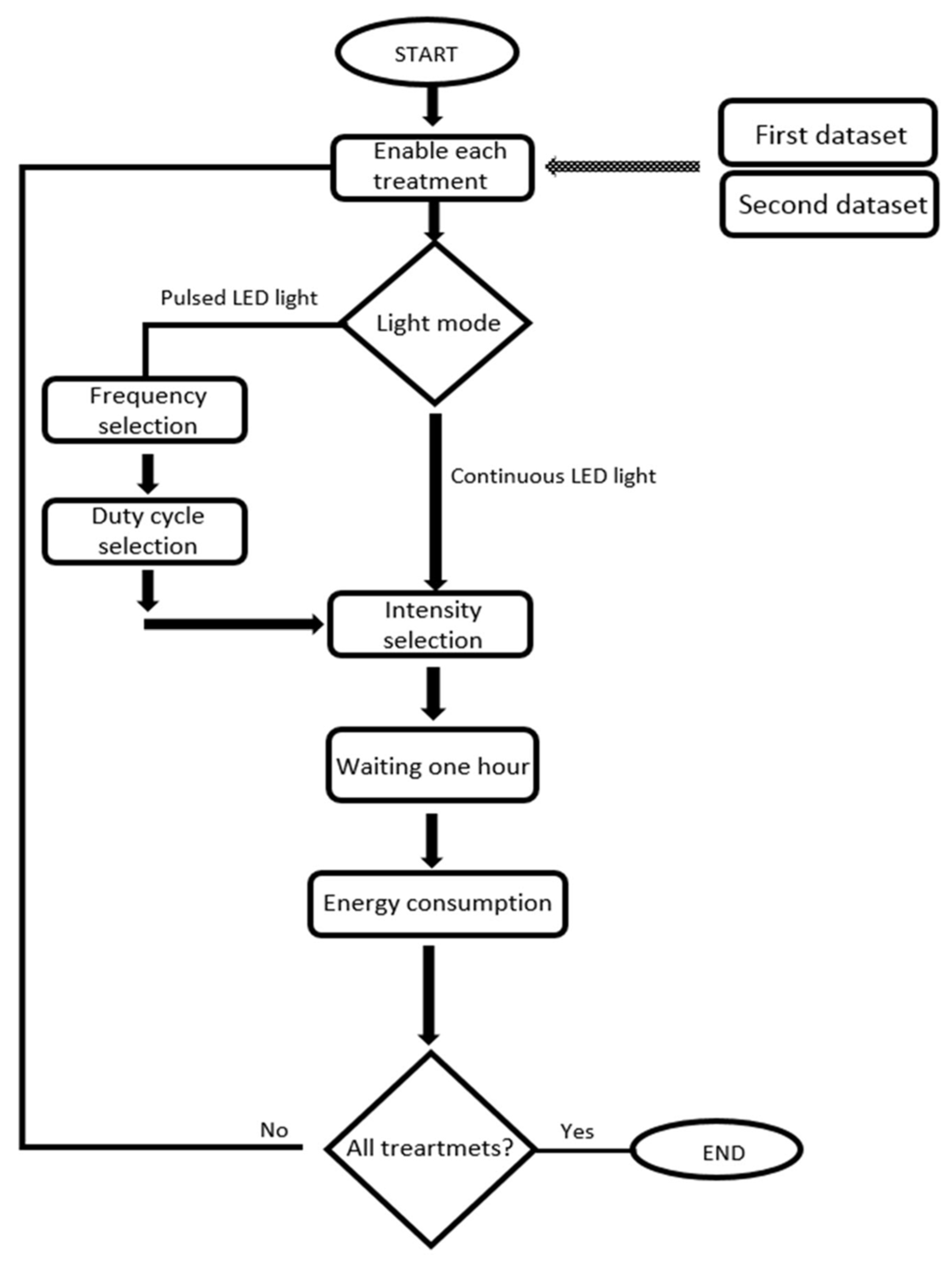
Two datasets for the generation and testing the GP and FNNs were applied. The first (Test 1) has 5700 samples with similar input ranges for training and evaluation; the second (Test 2) included a total of 160 datapoints in different input ranges from those used for training. The two models used energy consumption as output, while the inputs were intensity, red light component, blue light component, green light component, white light component, pulsed Frequency, and duty Cycle.
We normalized the first dataset to get its variables on the same scale.
Table 3 presents the slopes and offsets for normalization. Subsequently, the most relevant inputs in Test 1 were selected if Spearman’s
p value < 0.05 and
ρ ≥ 0.05, which implied a weak correlation with 95% reliability [
59].
Table 4 shows the correlation coefficients obtained using the inputs indicated in bold. After that, we split Test 1 as follows: 80% for the training and 20% for testing; meanwhile, Test 2 was also applied for testing in both models.
All the training stages for the GP and FNN models of this work were performed without parallel computing on a computer with Microsoft Windows 10.0.19041 Pro OS, Intel Core™ i7-6700 CPU with 3.40GHz, 16 GB RAM, and NVIDIA GeForce GTX 970 graphic card.
The GP training parameters selected with cross-validation were: SP = 200, ST = 20, and PM = 8%, for a limit of NG = 5000 generations. We avoided overfitting by selecting the complexity parameters (number of operations per parentheses and the number of parentheses) with 10-fold cross-validation in the training set. The best parameters obtained were 16 operators and 2 parentheses, with a cross-validation MAE of 3.0649, after testing 1−20 operators and 1−2 parentheses.
The GP model in the Equation (11) omitted input three (green light component), according to Spearman’s correlations in
Table 2.
We selected the complexity parameters of the FNNs model with 10-fold cross-validation obtaining three layers and 10 neurons per layer after testing 1–5 layers and 1–10 neurons, with a cross-validated MSE of 0.8666, and took 21,829.51 s or 6.06 h.
3.1. GP and FNNs Behavior in Test 1
The metrics for Test 1 with similar ranges to the training showed (
Table 5) that the GP model achieved 96.1% precision (1-MAPE), 3.90% MAPE, an average error between a real output value and a predicted one of 1.4384 watts (SEE), and 92.67% effectiveness at explaining the variability of the output variable (R
2). The MAE estimated for the GP model was 1.1239 and 3.0649 in the testing stage for the cross-validated MAE, i.e., a cross-validated error which was higher than the test error, which indicated a model without overfitting. In this context, the FNNs model obtained an accuracy or 1-MAPE, a MAPE, and the average errors between the real output value and a predicted one were 98.99%, 1.01%, and 0.4827 watts (SEE), respectively. The FNNs model effectively explains 99.34% of the variability of the output variable (R
2). The MSE for the ANN model was 0.3007 and 0.8666 in the testing stage for the cross-validated MSE, i.e., a cross-validated error higher than the test error, which indicated a model without overfitting.
Furthermore, FNNs showed slightly better performance than GP in the testing stage. The MAE and MSE levels were lower in FNNs, despite the training measures, as indicated in
Table 5.
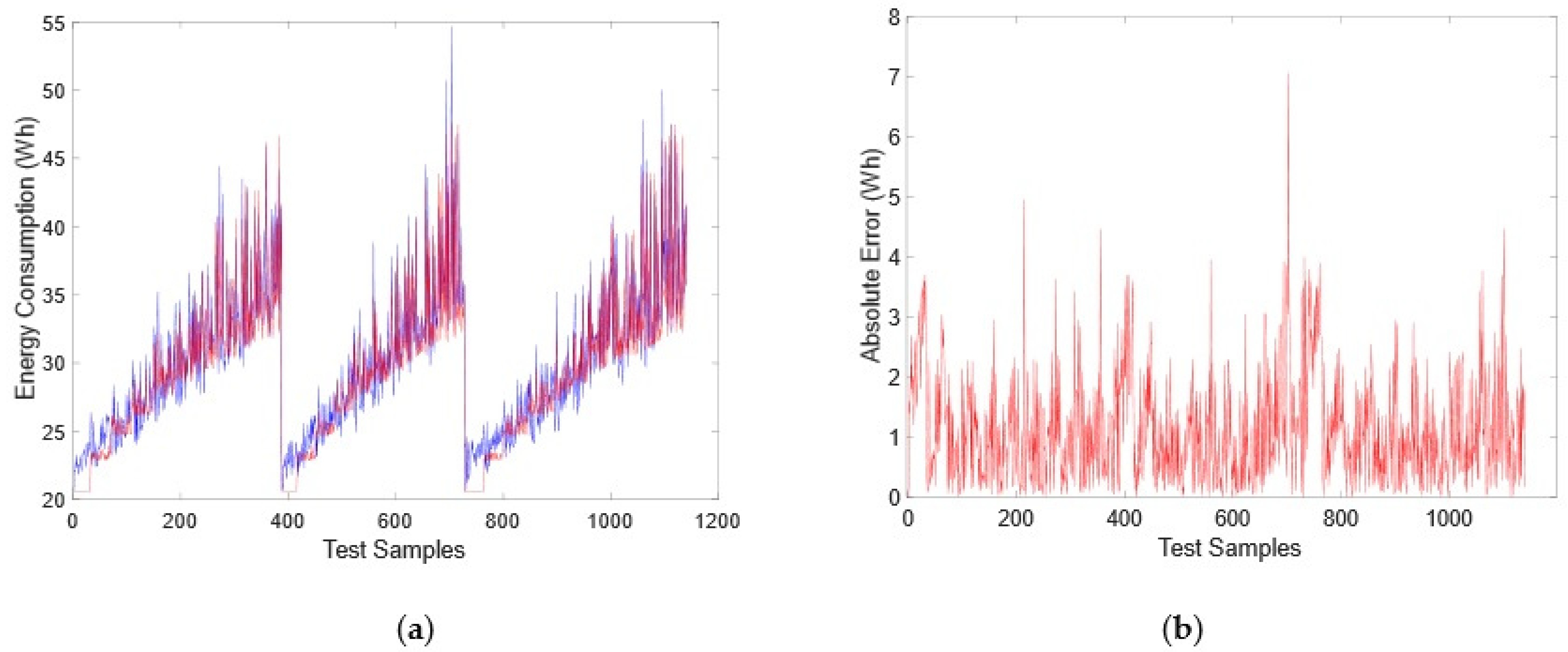
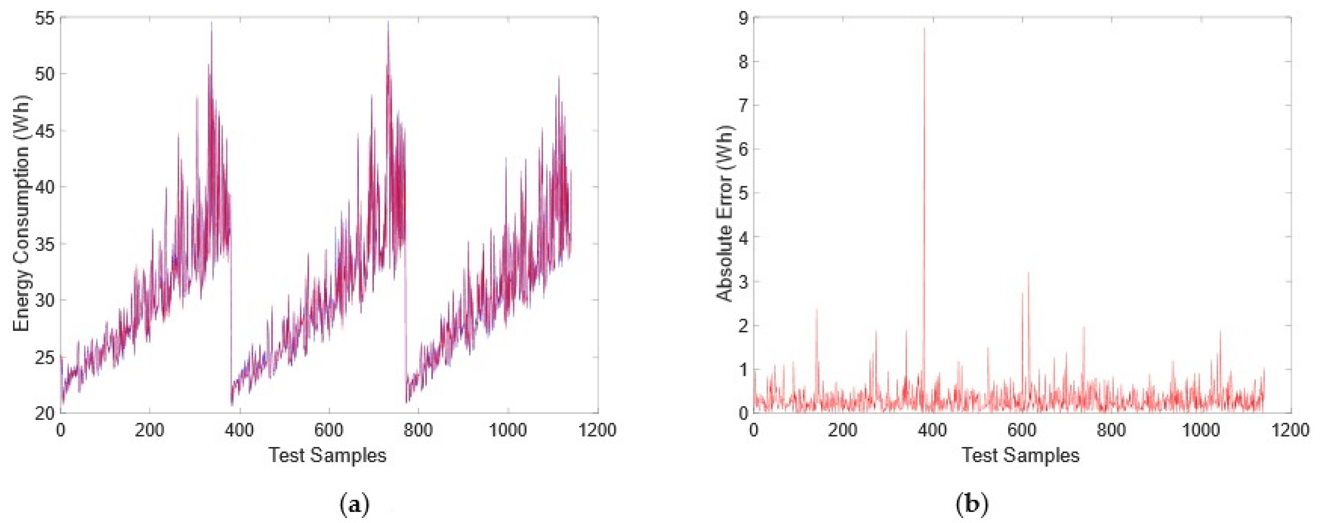
The GP model response (red line) and the desired output (blue line) are shown in
Figure 4a. The absolute error (AE) is plotted in
Figure 4b to identify the highest error per sample, i.e., 7 watts compared to 1.1239 watts of MAE.
The FNNs model response (
Figure 5a) exhibited a higher accuracy than the GP model, with finding a lower MAE, i.e., 0.3007, but a bigger punctual error that reached almost 9 watts (
Figure 5b).
3.2. GP and FNNs Models Behavior in Test 2
The accuracy metrics of Test 2 with different ranges to those used for training are shown in
Table 6. The GP model reached 95.35% accuracy, 4.65% error (MAPE); its average error (SEE) from a real output value to a predicted one was 1.8256 watts, which explains 83.99% of output variability (R
2). The FNNs model achieved 98.21% accuracy (1-MAPE) and 1.79% error (MAPE); the average error (SEE) between a real output value and a predicted one was 0.6776 watts, which explains 97.79% of the output variability (R
2).
The two datasets (Test 1 and Test 2) showed that the FNNs model was slightly superior to the GP model in the testing stage, despite the training measures. As shown in
Table 6, the error levels for MAE and MSE were lower in FNNs, while their effectiveness explaining the variable output variability or R
2 was superior.
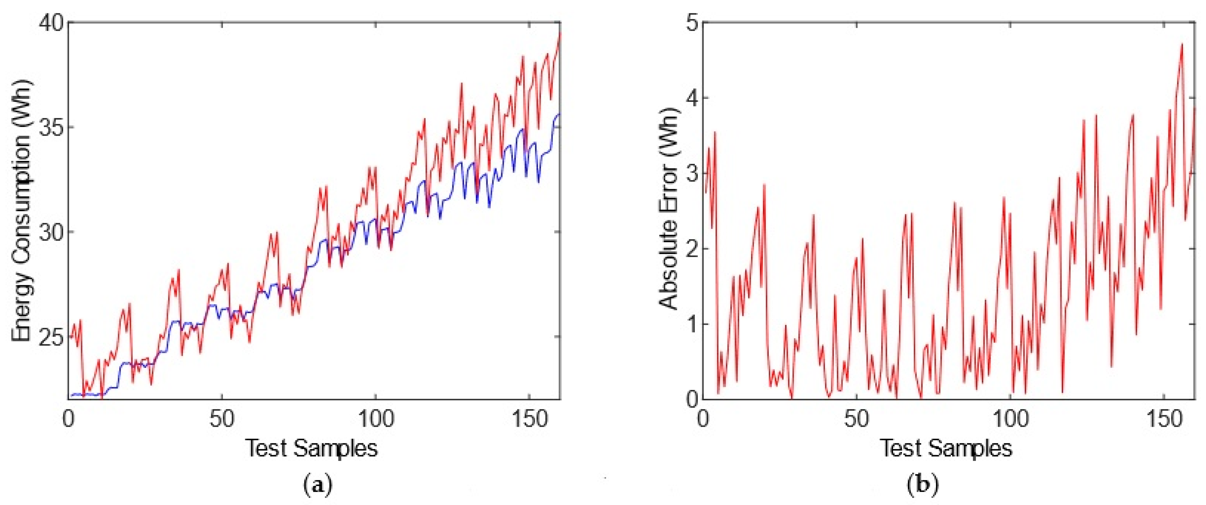
A comparative response between the obtained GP model output and the desired one (red and blue signals, respectively) is shown in
Figure 6a. We plotted AE in
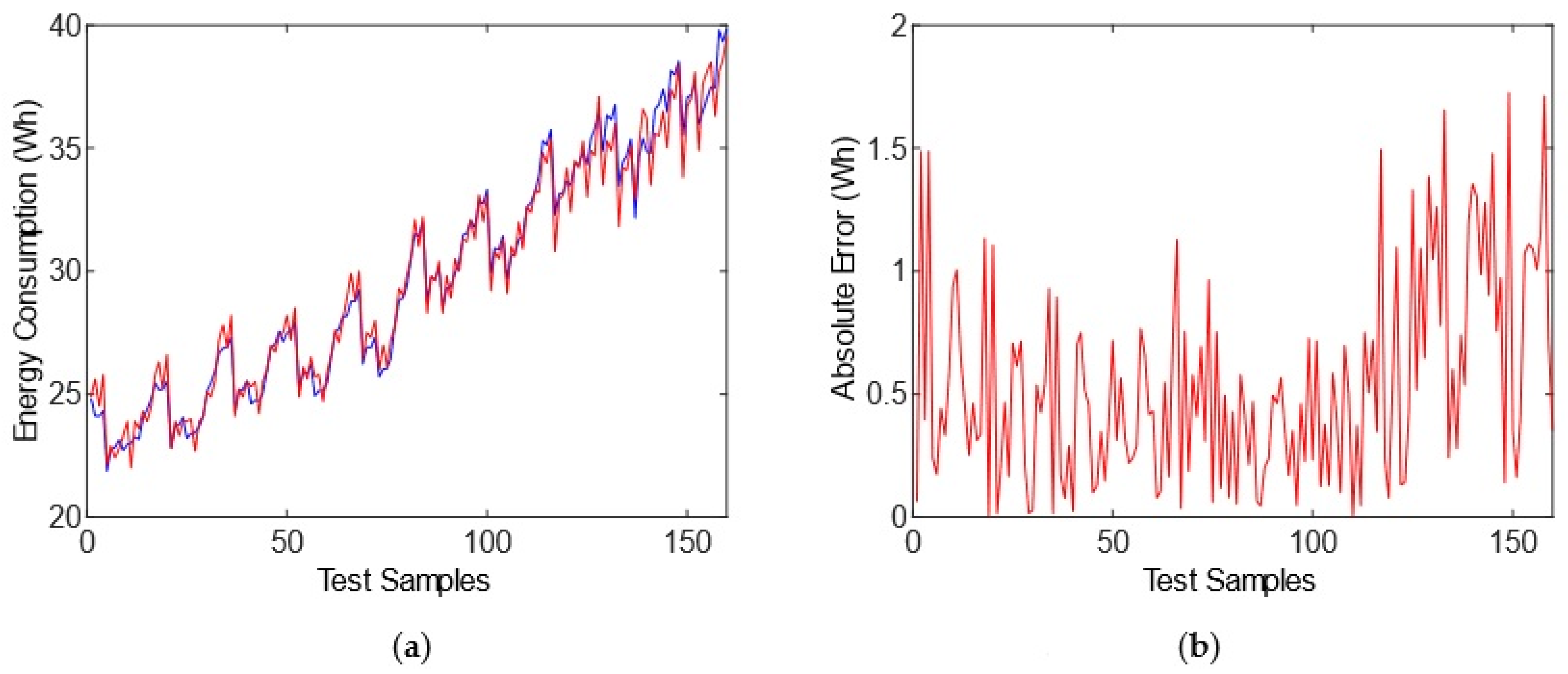
Figure 6b, showing a maximum error per sample of 4.6 watts, despite a MAE of 1.4508. The FNNs model response (
Figure 7a) exhibited a higher accuracy than the GP model, with a lower MAE of 0.5386, and presented a lower punctual error than the GP model, i.e., almost 1.8 watts (
Figure 7b).
3.3. GP and FNNs Models Statistic Comparison
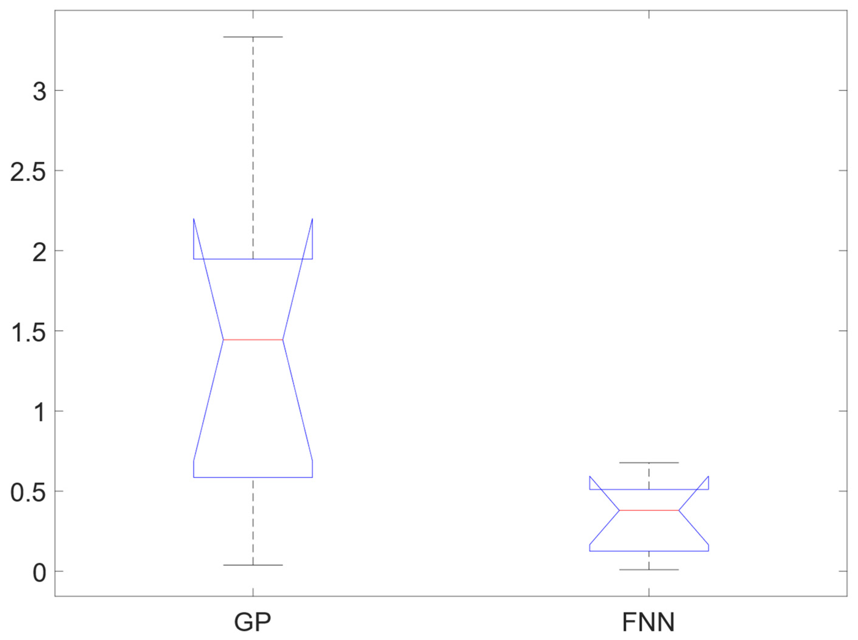
The estimated errors (MAE, MSE, SEE, and MAPE) for each nonlinear model (GP model and FNNs) in Tests 1 and 2 were integrated and associated with a new group of analyses (box plot and ANOVA). According to results obtained in the ANOVA and the graphic (box plot), it was determined that the FNNs model showed the best performance, considering the error and variance values, as observed in
Figure 8. Furthermore, the ANOVA with
supports these results, given that the established hypothesis (the error FNN < GP) is true with a 1.55% risk (
Table 7).
4. Conclusions
In this proposal, we compared two nonlinear models for predicting energy consumption in CPPS using a linear GP algorithm and FNNs. The models generated energy consumption as output, and took intensity, red light component, blue light component, green light component, white light component, pulsed frequency, and duty cycle as input variables.
We identified the most important variables with Spearman’s correlation. The accuracy achieved using similar test ranges to those used in training was 96.1% for the GP model and 98.99% for the FNNs. On the other hand, the accuracy achieved with different test ranges to those used in training was 95.35% for GP and 98.21% for FNNs. Test 2 indicated that FNNs had better generalization than GP.
We found that the FNNs model was superior to the GP model based on statistical tests R2, box plot, and one-way ANOVA with a risk probability of 1.55%. Additionally, FNNs trained faster (6.063 h), in terms of processing all the tested architectures, than GP, which required 169.274 h due to the high computational cost, as noted in the literature.
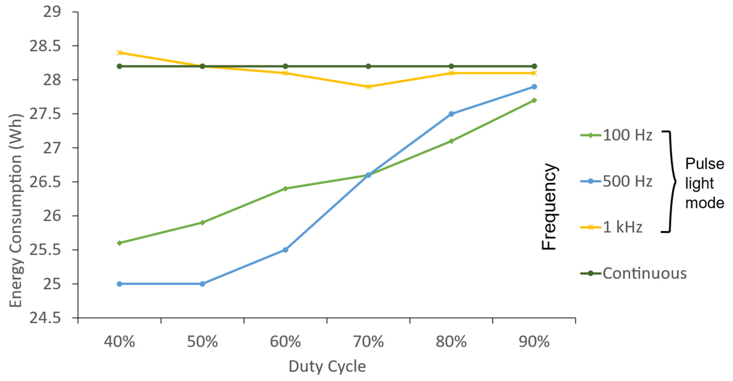
The GP and FNNs models generated in this proposal can be applied or programmed as part of a monitoring system for CPPS which prioritize energy efficiency. The results showed that the models achieved a forecast of energy consumption through a detailed analysis with each of the input variables. In this way, any new light recipe introduced in the literature or generated by the user generates a prediction about energy consumption. Projections of energy consumption are performed offline by moving the input parameters for both light operation modes (continuous and pulsed). The evaluation offered an advantage in several applications, as the pulsed light demonstrated energy savings through the application of different pulsed frequencies and duty cycles, compared with the continuous light. The proposed nonlinear models are directly connected to energy consumption predictions in real artificial radiation systems, so nonlinearities and parametric uncertainties were considered in the analysis. However, using new artificial lighting systems in CPPS implies retraining the model. However, once the models that describe the behavior of a lighting system have been trained, similar modules can be applied to cover a larger irradiation area without requiring remodeling. The proposed methodology serves as a reference for researchers, technicians, specialists, and entrepreneurs within the agro-industrial sector.


 ,
, 


