
Introducing Metamodel-Based Global Calibration of Material-Specific Simulation Parameters for Discrete Element Method


Endowed Chair of Construction Machinery, Institute of Mechatronic Engineering, Technische Universität Dresden, 01069 Dresden, Germany
*
Author to whom correspondence should be addressed.
Minerals 2021, 11(8), 848; https://doi.org/10.3390/min11080848
Submission received: 18 June 2021
/
Revised: 2 August 2021
/
Accepted: 3 August 2021
/
Published: 6 August 2021
(This article belongs to the Special Issue Simulation Using the Discrete Element Method (DEM) in the Minerals Industry)
Abstract
:An important prerequisite for the generation of realistic material behavior with the Discrete Element Method (DEM) is the correct determination of the material-specific simulation parameters. Usually, this is done in a process called calibration. One main disadvantage of classical calibration is the fact that it is a non-learning approach. This means the knowledge about the functional relationship between parameters and simulation responses does not evolve over time, and the number of necessary simulations per calibration sequence respectively per investigated material stays the same. To overcome these shortcomings, a new method called Metamodel-based Global Calibration (MBGC) is introduced. Instead of performing expensive simulation runs taking several minutes to hours of time, MBGC uses a metamodel which can be computed in fractions of a second to search for an optimal parameter set. The metamodel was trained with data from several hundred simulation runs and is able to predict simulation responses in dependence of a given parameter set with very high accuracy. To ensure usability for the calibration of a wide variety of bulk materials, the variance of particle size distributions (PSD) is included in the metamodel via parametric PSD-functions, whose parameters serve as additional input values for the metamodel.
1. Introduction
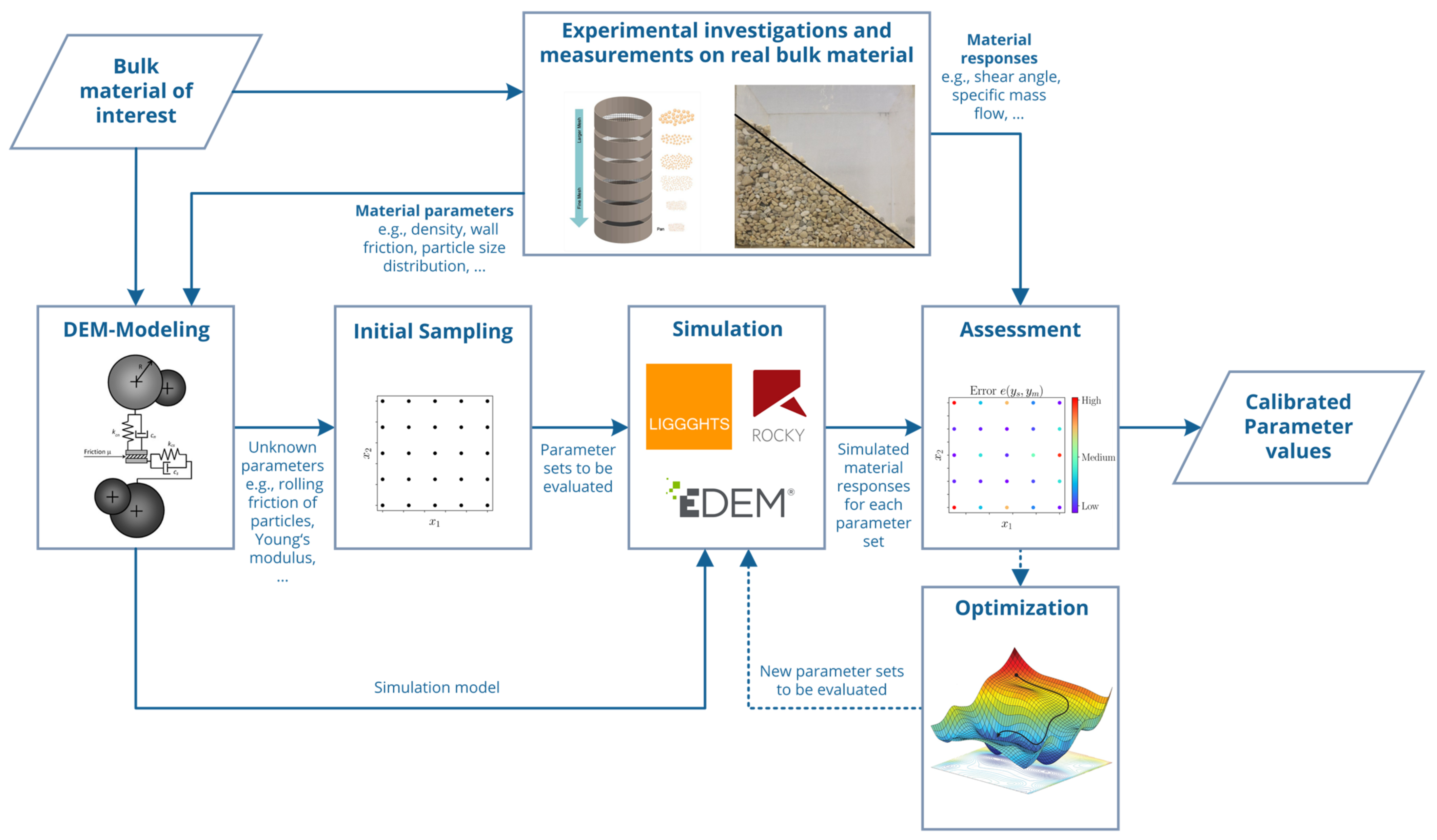
In recent years, discrete element method (DEM) has proven to be a suitable tool for simulating the behavior of different kinds of granular materials. Therefore, DEM is used in a wide range of industrial sectors, such as mining [1], construction machinery [2,3], agriculture [4], geotechnique [5], food industry [6] or pharmacy [7]. In addition to application-specific problems, all those who deal with DEM face the same problem at some point—the determination of the material-specific simulation parameters. These include particle density, particle shape and particle size distribution and the contact model parameters that define the interactions of the particles with each other or between particles and walls. While some of the parameters can be determined experimentally, e.g., particle size distribution in sieve analysis or coefficient of particle-wall friction in shear-cell test, the determination of others is rather difficult. The simple reason for this is that many contact model parameters are abstractions and simplifications of reality; thus, they have no physical counterpart and therefore cannot be determined by measurements. Typically, inverse parameter identification—also called calibration—is used to solve this issue. During calibration, a parameter set is sought for which the simulated material behavior corresponds as closely as possible to that of the real material. Figure 1 shows the scheme of a classical calibration approach.
Starting with experimental investigations on the real bulk material, measurable parameters as well as material responses are determined. Material responses are quantities that represent the macroscopic bulk material behavior in so-called calibration experiments, e.g., the well-known angle of repose in a cylinder test. The measured material parameters as well as the experimental setups are used to create simulation models replicating the calibration experiments. Subsequently an initial sampling will be created containing different parameter sets ; , where represents the number of unknown parameters respective to the number of dimensions. Generation of parameter sets can be done manually or automatically using different sampling strategies. Often full factorial designs or Latin hypercube samplings [8] are used. All parameter sets as well as the simulation models are passed to the DEM-Software, and simulations will be carried out. Afterwards, each parameter set is evaluated by an error function that compares the simulated material responses with the measured responses . The result of is called objective function value and should be minimized. If there is no parameter set leading to with acting as a user defined threshold for the acceptable error, new parameter sets will be generated by the user or an algorithm, trying to optimize respectively minimize .
Every parameter set generated during sampling- and optimization-phase corresponds to a DEM simulation, which may require several hours to days of computing time. Thus, total computational cost of calibration essentially depends on the number of necessary simulation runs, which can often be several hundred or thousand. In recent years, the focus of scientific investigations in this field of research has therefore been on reducing the number of simulations. In particular, new sampling methods and different optimization algorithms have been investigated, e.g., particle swarm optimization [2] or genetic algorithms [9]. Significant reductions on necessary simulation runs can be achieved especially by optimization algorithms which use the evaluated simulation results to train a metamodel, e.g., gaussian process models [10], kriging models [11] or artificial neural networks [12]. In literature, this is referred to as metamodel-based optimization (MBO). Metamodels, also known as surrogate models or response surface methodology, mimic the behavior of simulation models and can be used to predict a value for an unknown parameter set . The biggest advantage of metamodels is that most of them can be calculated in fractions of a second. MBO-algorithms use the results of the initial sampling to create an initial metamodel. Afterwards, an adaptive sampling strategy is used to search for new parameter sets, also referred to as points, which either improve model accuracy or minimize the estimated value of . Each new point is then simulated, and a new meta-model is built with the results.
Both, classical calibration in general and MBO in particular, still have some disadvantages:
- During initial sampling, a large number of parameter sets will be generated at once. Depending on the available computational resources, these parameter sets can be evaluated in parallel. Most metamodel-based optimization algorithms generate only one new parameter set per iteration, so the total time needed for calibration strongly depends on the number of necessary iterations during optimization phase.
- Each calibration sequence starts with an initial sampling. This is necessary to generate a minimum amount of initial information needed for the optimization algorithms, e.g., for training of initial metamodels. Even with continuous improvement of optimization algorithms as well as metamodel types, the minimal computational effort per calibration sequence is limited to simulations. Depending on the available computational resources as well as the simulation model, the time required for a calibration sequence can still take several hours to days.
- Simulation results as well as metamodels generated in one calibration sequence cannot be reused for other calibration sequences with new bulk materials. This has several reasons. First, most metamodels do not predict simulated material responses but objective function results . The objective function already contains the material-specific real material responses, which were previously determined in the course of experimental investigations. Another reason, which prevents the transferability of metamodels and simulation results to other bulk solids, is the fact that they are produced with discrete element models containing specific values for particle density, particle shape and particle size distribution. Thus, most metamodels are material-specific.
- The lack of reusability of metamodels as well as simulation results for other calibration sequences means that they are usually deleted immediately after the calibration sequence is completed. The only used output of a calibration sequence is the identified parameter set. If the output per calibration sequence is put in relation to the required time and computational effort, classical calibration has a very poor efficiency.
- Classical calibration aims at identifying a parameter set which leads to the desired material responses. Thus, it provides a punctual assignment between the input and output variables of the DEM simulation. The underlying effective relationships are not examined more closely and remain hidden. It is therefore a non-learning approach.
In the following metamodel based global calibration will be introduced, which solves the mentioned disadvantages.
2. Basic Idea of Metamodel-Based Global Calibration
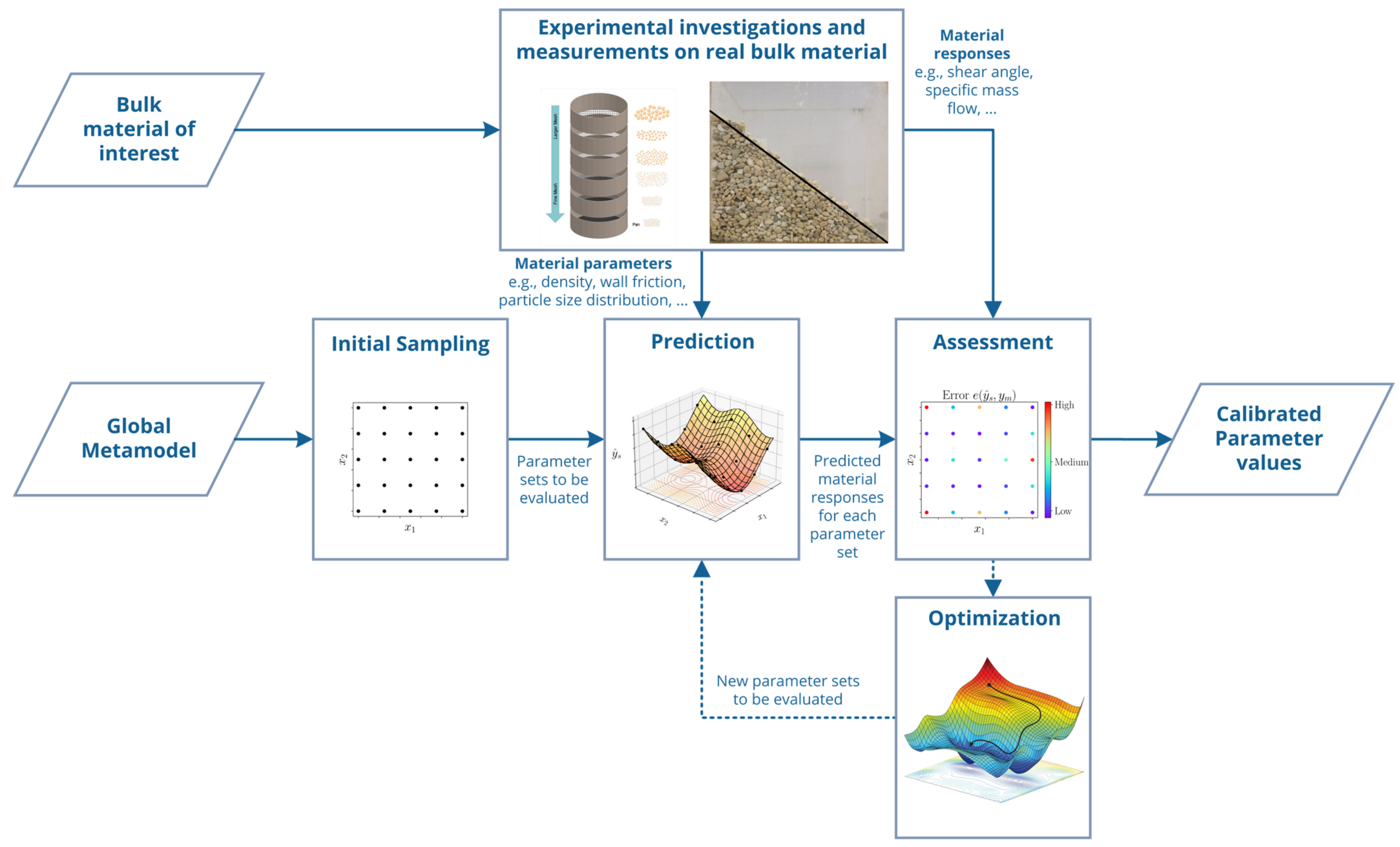
The basic idea of metamodel-based global calibration (MBGC) is to completely remove the time-consuming and expensive DEM simulations from the calibration process. This is done by using a global metamodel for predicting the material responses for unknown parameter sets as illustrated in Figure 2. Due to the omission of the simulations, the DEM modelling is also not part of the calibration sequence. The remaining steps are basically the same as in classical calibration approaches.
As mentioned before, MBO also uses metamodels for the prediction of material responses; therefore, it is important to point out that MBGC and MBO differ from each other in the way the metamodels are employed. MBO includes training and prediction of metamodels in the calibration process, while MBGC starts with an already existing metamodel. Furthermore, MBO uses DEM simulations in the calibration sequence, e.g., for calculation of points proposed by initial or adaptive sampling. In contrast to this, MBGC completely replaces the DEM simulations in the calibration sequence by metamodel predictions.
The term global in MBGC refers to the common differentiation between global and local metamodels [13]. While local metamodels are used to guide the optimization algorithm towards an optimum and are discarded afterwards [14], global metamodels provide a fast but accurate approximation of the behavior of the simulator on the entire domain [15]. Applied to the calibration of DEM models, this means local metamodels are able to predict the material responses for one bulk material, while global metamodels are suitable for the prediction of different bulk materials.
Central prerequisite for the calibration process is a global metamodel, which serves as an input value for the MBGC-algorithm. The metamodel must be created beforehand which requires an initial one-time effort. Subsequently, the metamodel can be used for the calibration of different bulk materials. The process of global metamodeling should be explained below.
3. Global Metamodeling
Success of MBGC strongly depends on the metamodel used. In the following, the different steps in the process of global metamodeling shall be briefly explained.
3.1. Material Domain
First of all, the user has to define which kind of materials the future metamodel should represent. The specification of certain material properties and limits defines the boundary conditions under which the metamodel can be used later and forms the so-called material domain. It should be clear that the more generalized the specification of a material domain is, the larger is the range of materials it covers and the higher the utility of the future metamodel. For this, the specification requires a certain level of abstraction and interdisciplinary thinking by the user, because usually material range is not fixed to one industrial sector. The delimitation of the material domain as well as the specification of the material range it covers is hard to define. It is helpful to first outline the domain qualitatively with the help of a simple description. This description should contain important bulk material properties under consideration as optionally some industrial sectors to get an imagination who could use the later metamodel. For example, the material domain, which should be investigated below, is defined as follows: “Non-cohesive bulk materials from mining, construction industry and natural materials technology”.
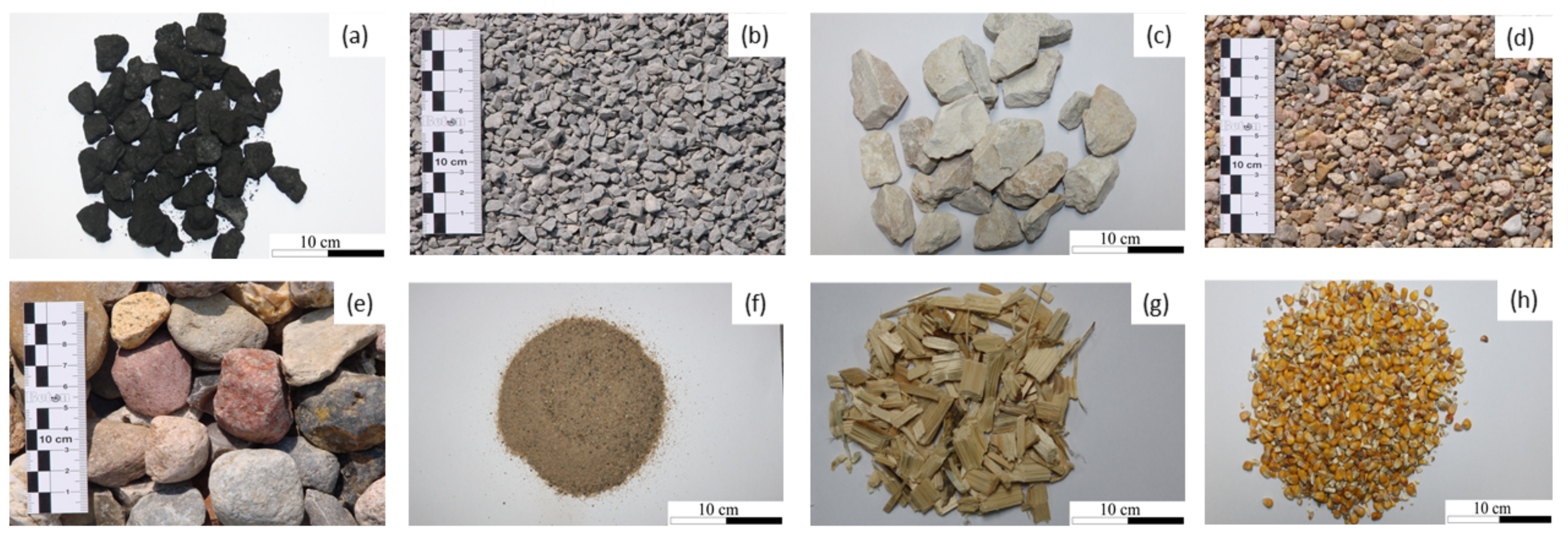
In order to quantify the domain boundaries, it is useful to supplement this admittedly very vague description with some example materials. Hence, different materials from mining (coke, hard coal, limestone) and construction industry (gravel 2/8 mm, gravel 16/32 mm, dry sand) as well as from natural materials technology (woodchips, dry corn) were chosen (Figure 3).
3.2. Contact Model
After some example materials have been chosen a contact model should be defined, which is able to describe this range of materials. As mentioned above, the material domain covers only non-cohesive materials. For this, a Hertz–Mindlin-model with no cohesion will be used. As an idealization, all particles are considered as spheres. To account for the fact that some particles have a shape that is far away from spherical a modified elastic plastic spring dash pot model (EPSD) according to Wensrich [16] will be used to calculate rolling friction. It should be mentioned that the future metamodel can only be used in conjunction with this contact model. The used contact model is kind of a standard model, which is implemented in many software tools. The DEM software which is used here is LIGGGHTS-PUBLIC 3.8.0 [17].
3.3. Parametric Particle Size Distribution
An essential novelty of MBGC is to consider the particle size distribution (PSD) as an additional input for the metamodel. This is the key to represent different materials, which usually have different particle size distributions. A major challenge in this context is the appropriate parametric representation of particle size distributions. Usually, the PSD of a material is described by discrete pairs of values , where is the particle diameter of fraction and is the associated cumulative mass fraction. The corresponding values are determined, for example, in the course of a sieve analysis. An obvious way to include the PSD in the metamodel is to use these values as additional input parameters. One major drawback of this variant, is that it results in a relative high number of inputs. For a usual number of fractions, this results in additional parameters. This is unfavorable, because the number of training data sets strongly depends on the number of input parameters. For this reason, analytical distribution functions should be used here.
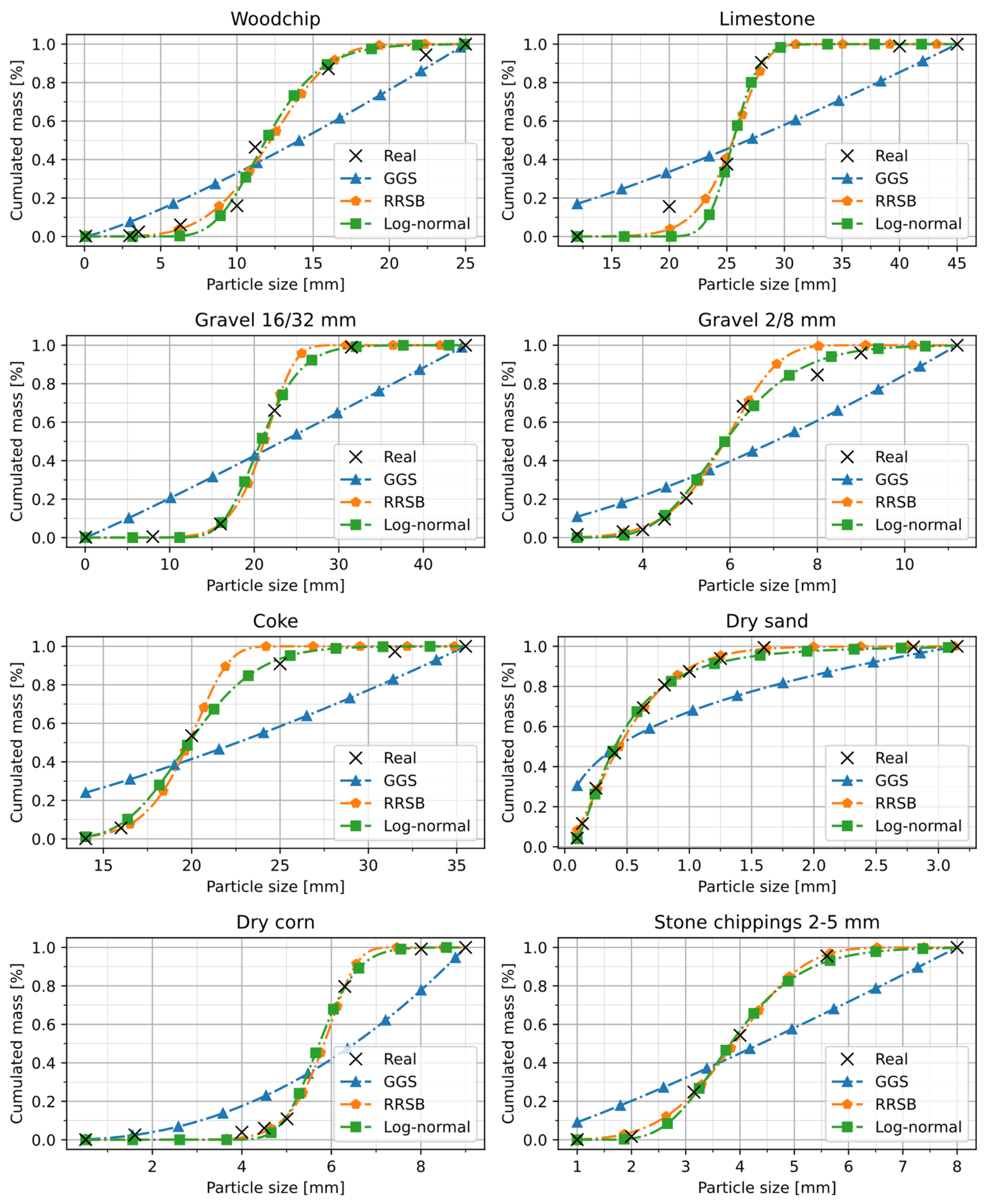
In literature, there are different distribution functions that could be used for the description of particle size distributions. Among the best known are Rosin–Rammler–Sperling–Bennet (RRSB), Gates–Gaudin–Schumann (GGS) and the Lognormal-distribution (LOGN) (Equations (1)–(3)). All these functions are two-parametric, which means only two additional inputs are used for the metamodel.
To find out which distribution function should be used, all of them have been fitted to the real PSD-data of the example materials. Fitting was done using linear least squares approach. Figure 4 shows the results. For comparison the coefficient of determination as well as the mean squared error between the real data and the fitted curves have been calculated (Table 1). The results show that GGS-function provides worst results for all materials considered. LOGN as well as RRSB approximate the real particle size distributions very accurate, while Log-normal distribution delivers slightly better results and therefore should be used for this material domain.
3.4. Definition of Parameter Space
Next, the parameter space must be defined, containing the lower and upper boundaries for all input parameters of the metamodel. The parameter space is a quantification of the material domain defined above. Table 2 shows all parameters used in the following. The lower and upper boundaries for and are results from the fitting process, while other parameters are limited to reasonable values based on experience and theory behind.
3.5. Calibration Experiment and DEM-Modeling
The next step is to select or devise a calibration experiment. Global metamodeling places some demands on the experimental design, which should be considered. Since several hundred simulations have to be carried out to obtain enough training data for an adequate metamodel, the experiment should be simple and small-scale in order to compute it within a short time. The use of a parametric particle size distribution leads to a varying number of particles in the simulation. In order to keep the number of particles as well as the computing time per simulation approximately the same, the experiment should be scalable and the extracted features scale-invariant. This means if the particle size is increased, the geometric shapes should be downscaled too, but the extracted results, e.g., the angle of repose, should not be affected by this. Furthermore, the experimental design should be robust and reliable. This means that for each parameter combination, the experiment should have the expected course. The problem of a potentially unrobust experiment can be illustrated by the example of a silo outflow. Due to the varying parameter values, e.g., for coulomb and rolling friction, bridging can occur in some simulations, which leads to no measurable angle of repose under the silo. This would lead to no or invalid results for some parameter sets. One possibility to make this kind of experiment more robust is to choose the silo opening large enough to avoid bridging in all cases.
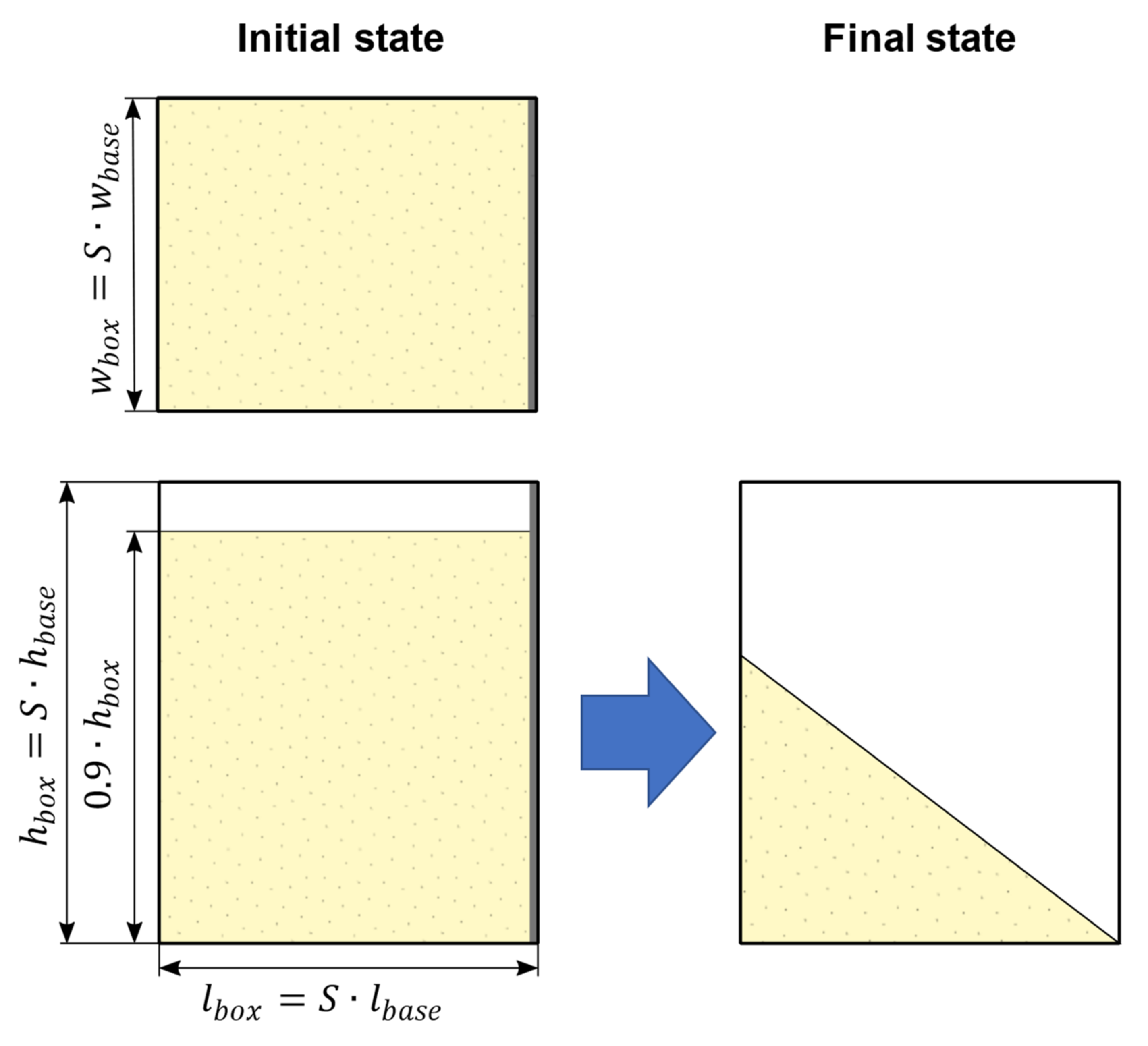
In the following, the shear box test proposed by Rössler et al. [18] was used. In this experiment, a box is filled with material, and then, one side is opened so that the material can flow out. Figure 5 shows the geometric setup of the experiment.
The basic dimensions of the original experiment were modified and given a scale factor , which depends on the maximum particle diameter and the minimum side length of the basic box geometry defined by , and . Equation (4) shows the calculation of , which ensures that smallest dimension of the box is ten times the maximum particle diameter.
Moreover, the simulation time step depends on the current parameter values and must be calculated for each simulation. As suggested by Thornton [19], the Rayleigh wave speed can be used to determine the critical time step for non-linear contact models such as Hertz–Mindlin. The following expression for the Rayleigh time step is given by Li et al. [20].
The time step used for simulation is a fraction of as defined by Boac et al. [21].
3.6. Sampling Strategy
The data used for metamodel training, i.e., the parameter sets and corresponding features, are of crucial importance for future model accuracy. The choice of a suitable sampling strategy used to generate the parameter sets is therefore at least as important as the choice of a metamodel type. As mentioned by Liu et al. [22], sampling approaches can be classified into two categories: one-shot sampling and sequential sampling. One-shot sampling approaches determine the sample size and points in a single stage. Well-known representatives are full factorial designs as well as Latin hypercube designs. One-shot approaches are unsuitable if no prior knowledge about the target function is given and an optimal or appropriate sample size cannot be predetermined. In this case, sequential approaches should be used, which sequentially determine new points using the information from previous iterations.
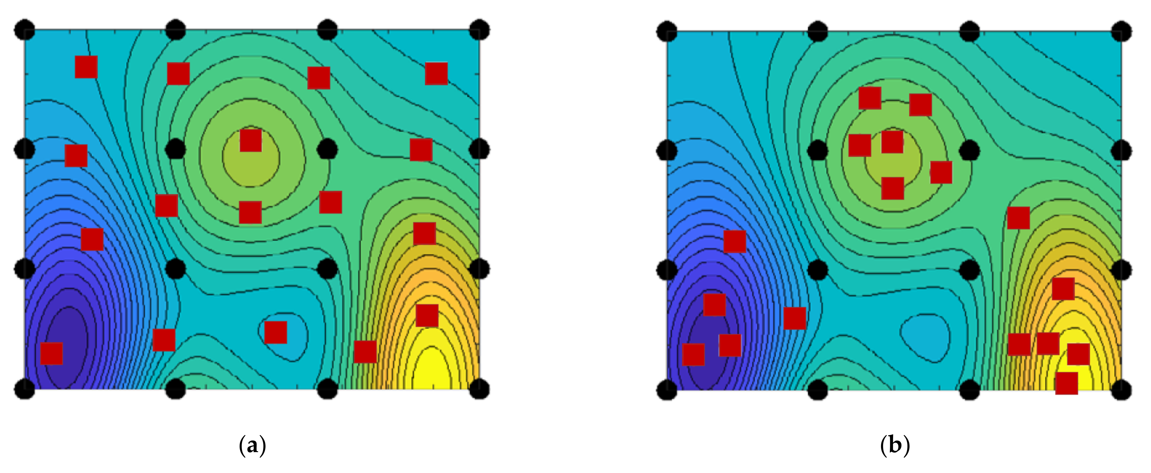
Sequential sampling approaches can be subdivided into two categories—space-filling sequential sampling and adaptive sequential sampling (Figure 6). Space-filling approaches try to fill the space between the points iteratively and spread the generated points over the entire parameter space. Adaptive approaches attempt to improve the accuracy of the metamodel by incorporating information about the metamodel into the generation process for new points. Subsequently, adaptive strategies as well as the resulting sampling are not model independent and should not be used to train different metamodel types. For this reason, in the following, only space-filling sequential sampling is investigated.
A popular group of sequential space-filling strategies are low discrepancy sequences, also known as quasi-random sequences. These methods are deterministic and obtain a uniform distribution of points based on discrepancy criteria. Discrepancy is a measure of the distance between an empirical distribution of points and a theoretically uniform distribution. Examples are Halton sequences [24] or Sobol Sequences [25]. Alternatives to low discrepancy sequences are the fully sequential space-filling design algorithm (FSSF-f) proposed by Shang and Apley [26] and the Monte Carlo-Intersite-proj-th (MIPT) algorithm proposed by Crombecq et al. [15].
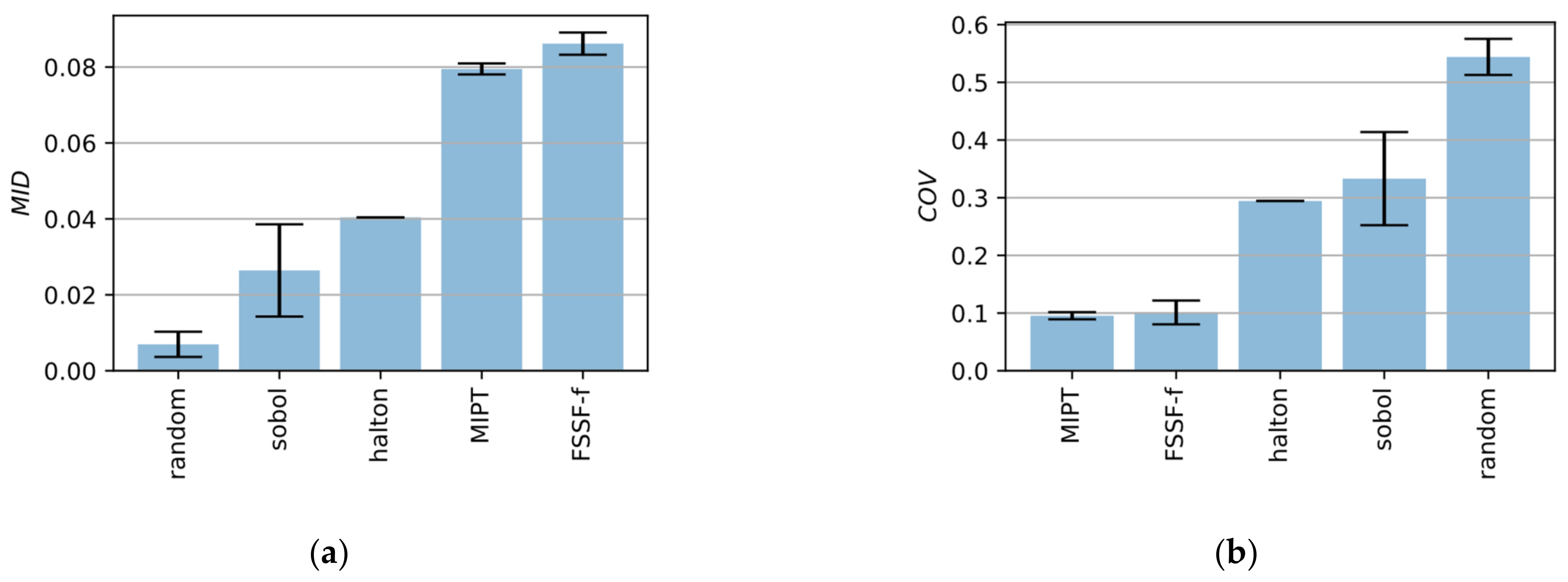
For the comparison of the different methods, metrics for the evaluation of the space-filling properties as well as the uniformity of the sampling are necessary. One of the most used criteria is the maximin-criterion also referred to as minimum intersite distance (MID) (Equation (7)). High values of MID correspond to a good space-filling.
Another metric is the cover measure (COV) [27]. Low values of COV correspond to a distribution close to a regular grid and ensure that the points fill up the space.
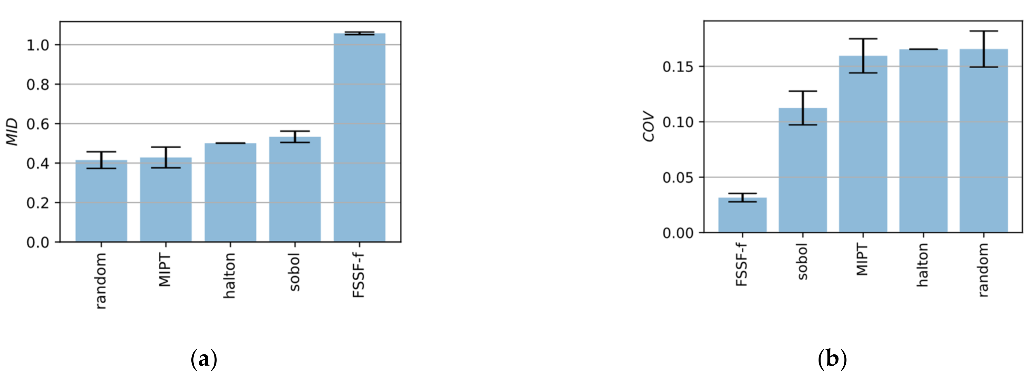
To benchmark the different sampling strategies all methods, including a purely random sampling, were used to create 100 points in a 2-dimensional as well in a 10-dimensional parameter space. This process has been repeated 10 times with different initial seed values for the algorithms. Box plots in Figure 7 and Figure 8 show the results.
It can be seen that the FSSF-f algorithm gives by far the best results leading to high values for MID as well as low values for COV. While MIPT also performs very well for 2-dimensional space, the algorithm delivers poor results in high dimensional space. that is why, in the following, the FSSF-f algorithm is used.
3.7. Metamodel
Various types of metamodels can be found in literature. Among the most popular ones are linear and polynomial regression models, artificial neural networks, support vector machines, radial basis functions, kriging or gaussian process models. All of these have advantages and disadvantages, which makes the selection of a suitable model type quite difficult. For this purpose, it is necessary to list the most important requirements for metamodels used for MBGC.
3.7.1. Choice of a Metamodel
First of all, a suitable metamodel should be appropriate for global approximation. Local approximation techniques, such as linear and quadratic polynomial regression, can therefore be excluded. Other important requirements are interpretability and introspective properties. A large number of metamodel-types can be seen as kind of a Blackbox. Such models allow the prediction of values but do not provide deeper insights into the functional relationships between the input and output variables. Last but not least, a suitable metamodel should have extrapolative properties making it possible to predict the results for parameter sets laying beyond the secured parameter range.
In the following, a meta-modelling technique is used which fulfils all requirements. This technique is called Symbolic regression (SR). Symbolic Regression is a type of regression analysis that searches the space of mathematical expressions to find an expression that best fits a given dataset, both in terms of accuracy and simplicity. Contrary to other regression techniques, such as linear or non-linear regression, no particular model is provided as a starting point to the algorithm. Instead, initial expressions are formed by randomly combining mathematical building blocks such as mathematical operators, analytic functions, constants and state variables. By not requiring a specific model to be specified, symbolic regression is not affected by human bias or unknown gaps in domain knowledge. There are different methods and algorithms for performing symbolic regression. Besides lesser-known methods such as Prioritized Grammar Enumeration [28] or Deep Symbolic Regression [29], the most popular one is Genetic Programming (GP), which is used in the following. The basics of genetic programming should be explained briefly below.
3.7.2. Genetic Programming
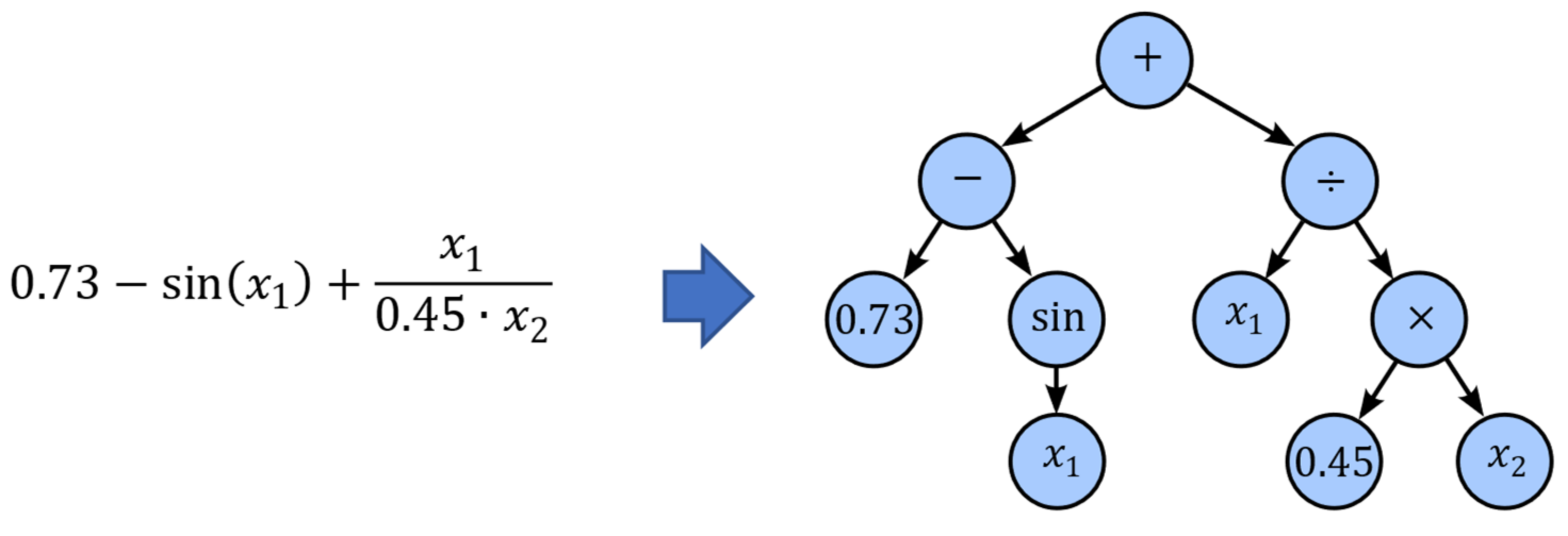
The basic idea of genetic programming is based on the fact that functions can also be represented as tree structures also called expression trees (Figure 9). Internal nodes of an expression tree contain mathematical operators while terminal nodes contain the operands, e.g., constants and variables.
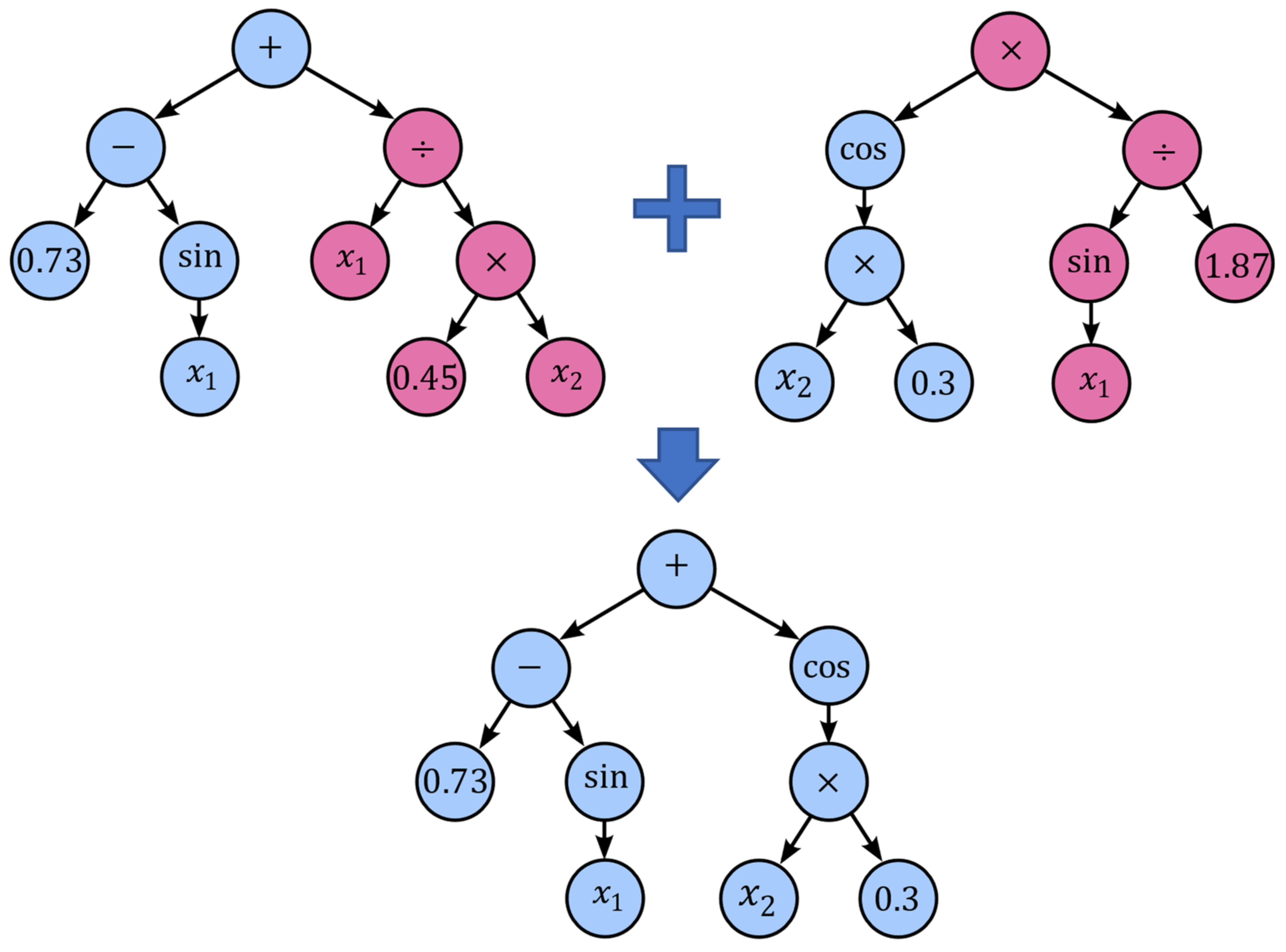
At the beginning of a genetic programming sequence, several expression trees are generated by randomly choosing and combining different mathematical operators, constants and variables. Thereby, the mathematical operators are drawn from a predefined function set . Every expression tree can be seen as an individual of a population . Afterwards, a fitness value is assigned to each individual, representing how good the corresponding function fits the data. Typical metrics for calculating are the well-known mean squared error or root mean squared error. Subsequently, the GP algorithm uses the basic principles of evolution, namely, selection, recombination and mutation, to gradually create new generations of individuals. Each new generation of expression trees is evolved from the one that came before it by selecting the fittest individuals from the population in a tournament and recombine them. This process of mixing genetic material between individuals is called crossover (Figure 10). Additionally, to crossover different kinds of mutation are used to maintain genetic diversity from one generation to the next.
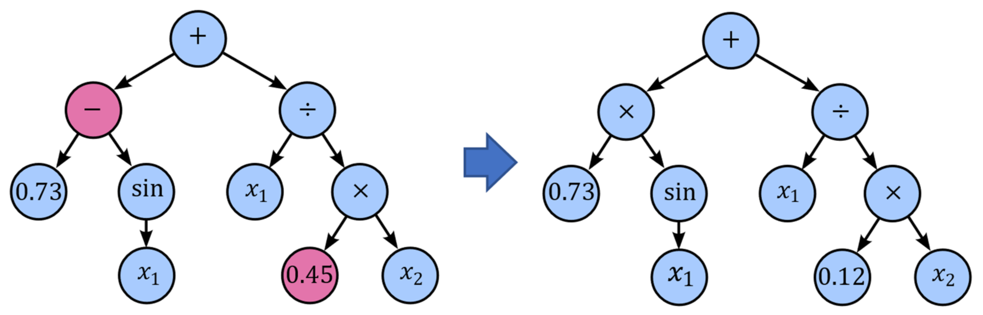
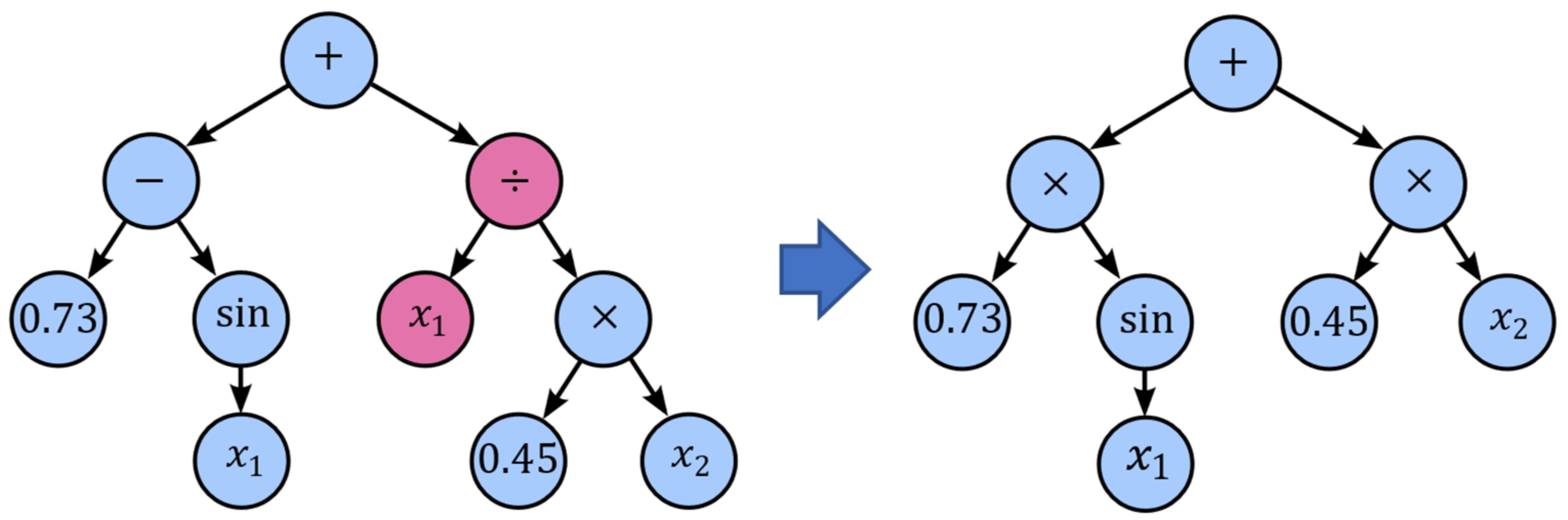
Point mutation is probably the most common mutation method in genetic programming, which takes the winner of a tournament and selects random nodes from it to be replaced. Terminals are replaced by other terminals, and operators are replaced by other operators that require the same number of operands as the original node (Figure 11). The purpose of point mutation can be used to reintroduce extinct functions and operators into the population to maintain diversity.
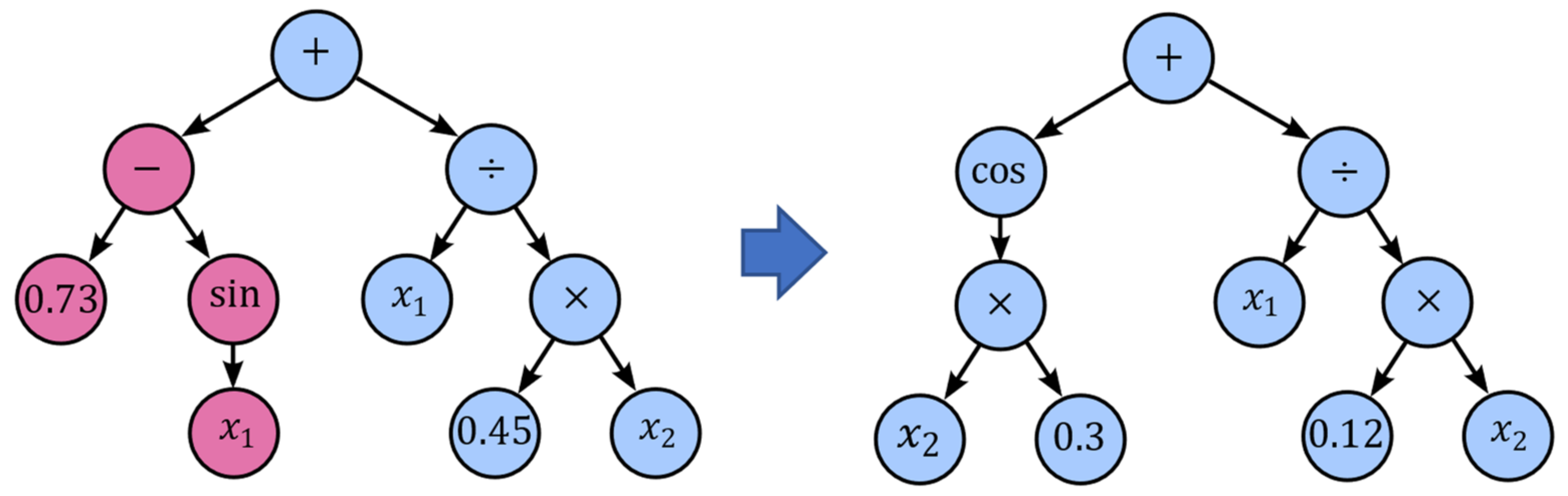
Another mutation technique is subtree mutation, which can also be used to maintain diversity (Figure 12). Subtree mutation takes the winner of a tournament and selects a random subtree from it to be replaced by a donor subtree, which is generated randomly.
Crossover and subtree mutation may lead to expression trees growing larger and larger with no significant improvement in fitness. This phenomenon is called bloat. One effective method to counteract the growth of expression tress is hoist mutation. Hoist mutation takes the winner of a tournament and selects a random subtree from it (Figure 13). A random subtree of that subtree is then selected and “hoisted” into the original subtree’s location. In this way, genetic material is removed from the expressions.
Another way to fight bloat is the use of a penalized fitness measure where the fitness of an individual is made worse the larger the corresponding expression tree is. The length of an expression tree can easily be determined counting the number of nodes. The penalty and thus the intensity with which bloat is controlled depends on the so-called parsimony coefficient.
For genetic programming the software package gplearn [30] is used. Population size is set to 5000 individuals, and a parsimony coefficient of is used. The function set is , which includes the most important mathematical operators and functions except trigonometric functions. Trigonometric functions, e.g., , and , have been excluded from the function set because it can be assumed that there is no periodically repeating behavior. Furthermore, it was found that usage of these functions could lead to overfitting.
4. Results
4.1. Global Metamodelling
In this section, the results of the metamodeling process shall be presented. For training of the different metamodels, 563 parameters sets generated by FSSF-f algorithm have been used. Originally, 600 simulations have been carried out, but some results were discarded because of simulation crashes. Validation of model accuracy was done using a second dataset with 68 parameter sets generated by a random sampling method. The considered response variables are the shear angle and bulk density . Response variables are obtained automatically using the output data of the simulations. For determination of the shear angle, the coordinates of all particles are evaluated at the end of the simulation, and a linear regression is performed through uppermost particles. Calculation of bulk density is based on the mass of the particles in the box after filling as well as the volume of the box.
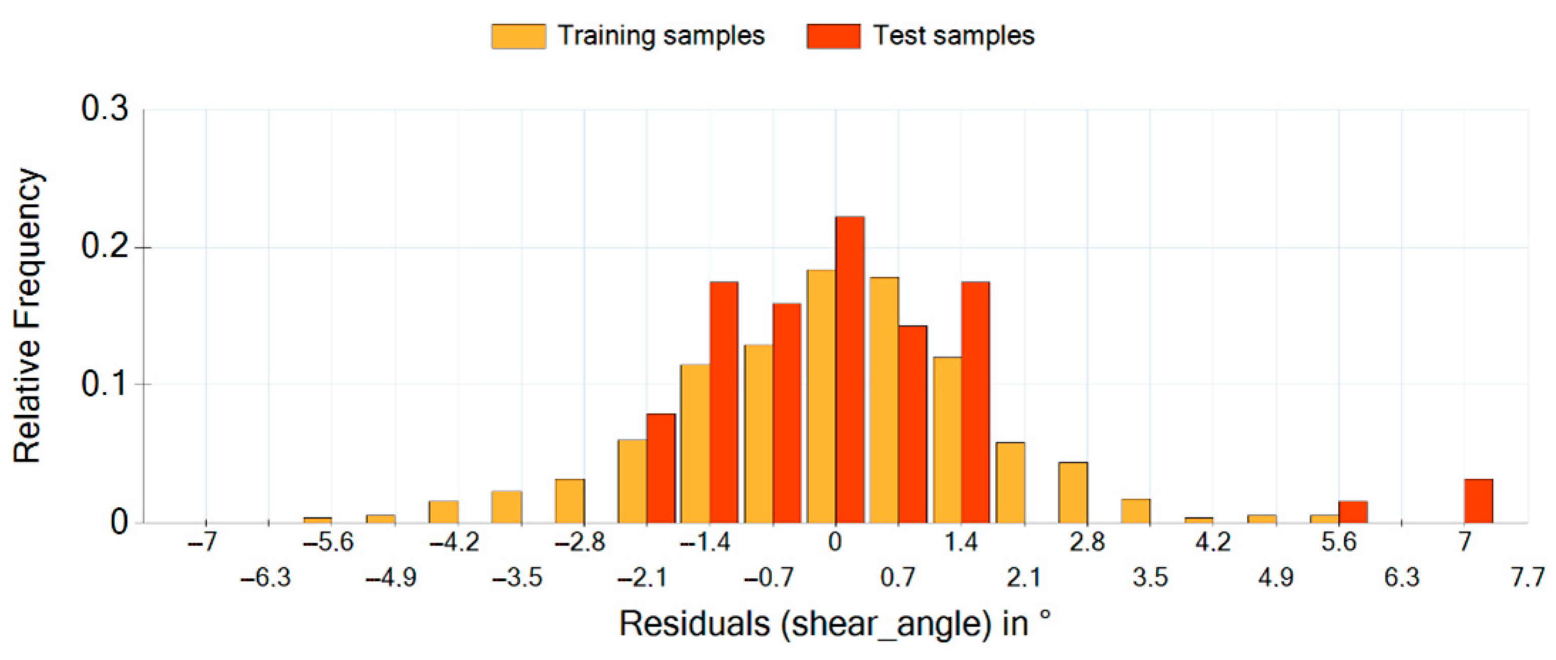
Equation (9) shows the final analytical solution for shear angle estimation. The corresponding residuals between the estimated values and the training samples respectively test samples are shown in Figure 14.
It can be seen that not all of the 12 variables considered in Table 2 are included in Equation (6). This is due to the property of genetic programming that variables with little influence on the results are eliminated by the evolutionary process sooner or later. This means GP implicitly performs a sensitivity analysis and variable selection. This makes analysis of the parameter effect very easy.
The shear angle is influenced by the parameters , , , , and . It is immediately apparent, for example, that the shear angle is not influenced by particle scaling, which would lead to changes in . Moreover, it does not depend on young’s modulus, Poisson ratio or particle density. The histogram values show that most of the estimated values have a residual between −1.4° and 1.4°, which is very accurate. The coefficient of determination for this model is 0.98085. The outliers on the right side of the histogram can be attributed to inadequacies in shear angle calculation, which will be explained more in detail in Section 4.
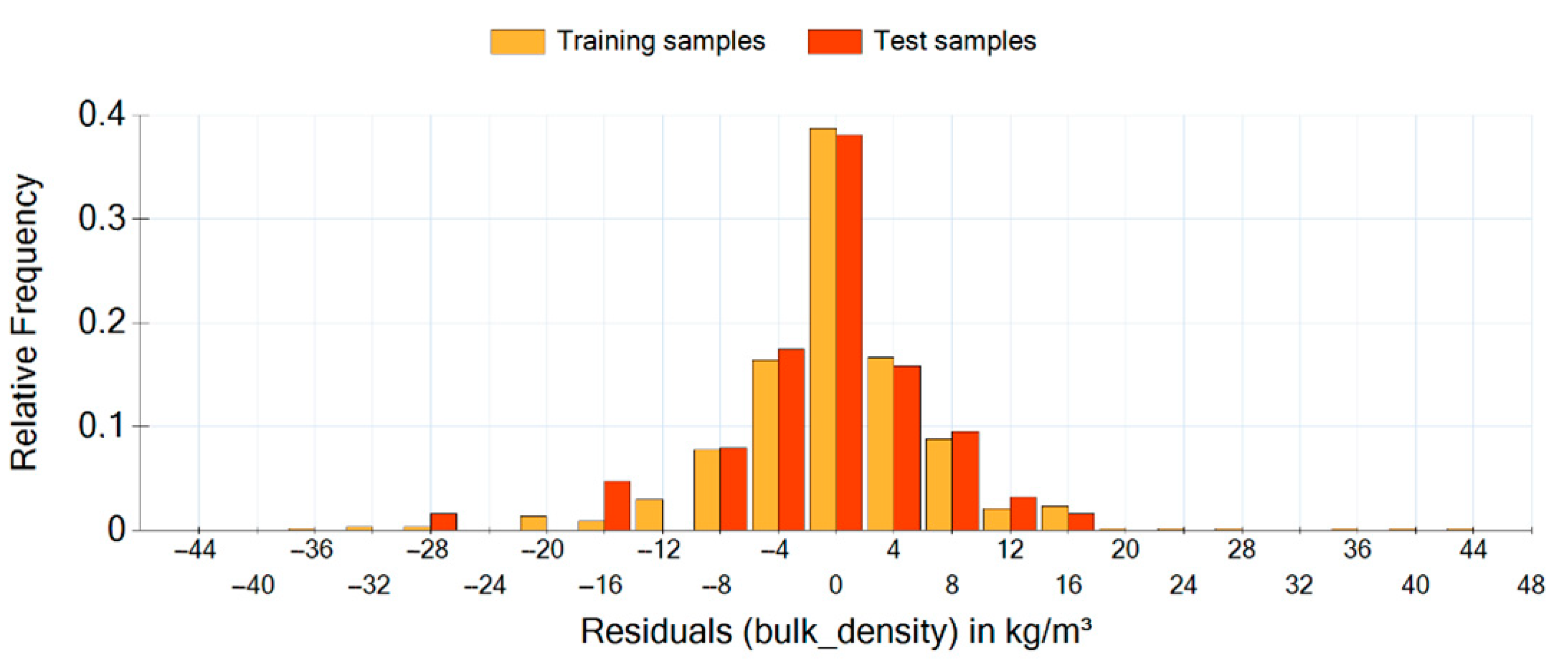
Equation (10) shows the analytical solution for bulk density estimation. The bulk density results from the mass in the box divided by its volume. The corresponding residuals between the estimated values and the training samples respective test samples are shown in Figure 15.
It is recognizable again that not all parameters have an influence on the bulk density. Bulk density is influenced by the parameters , , , , , , and . Even if the absolute values of the residuals seem to be very large, they are very small considering the large range of values for bulk density starting from 100 kg/m³ and going to 2000 kg/m³. With a determination coefficient of 0.99975, the prediction accuracy of this model is quite better than that of shear angle estimation.
The equations above show that it is sometimes unpredictable which parameters have an influence on the response variables and which not. For example, it is not easy to understand neither to explain why an influence on bulk density but not on shear angle has. Interpretation of the equations generated by MBGC is a separate task and not topic of this research paper.
4.2. Parameter Identification and Validation
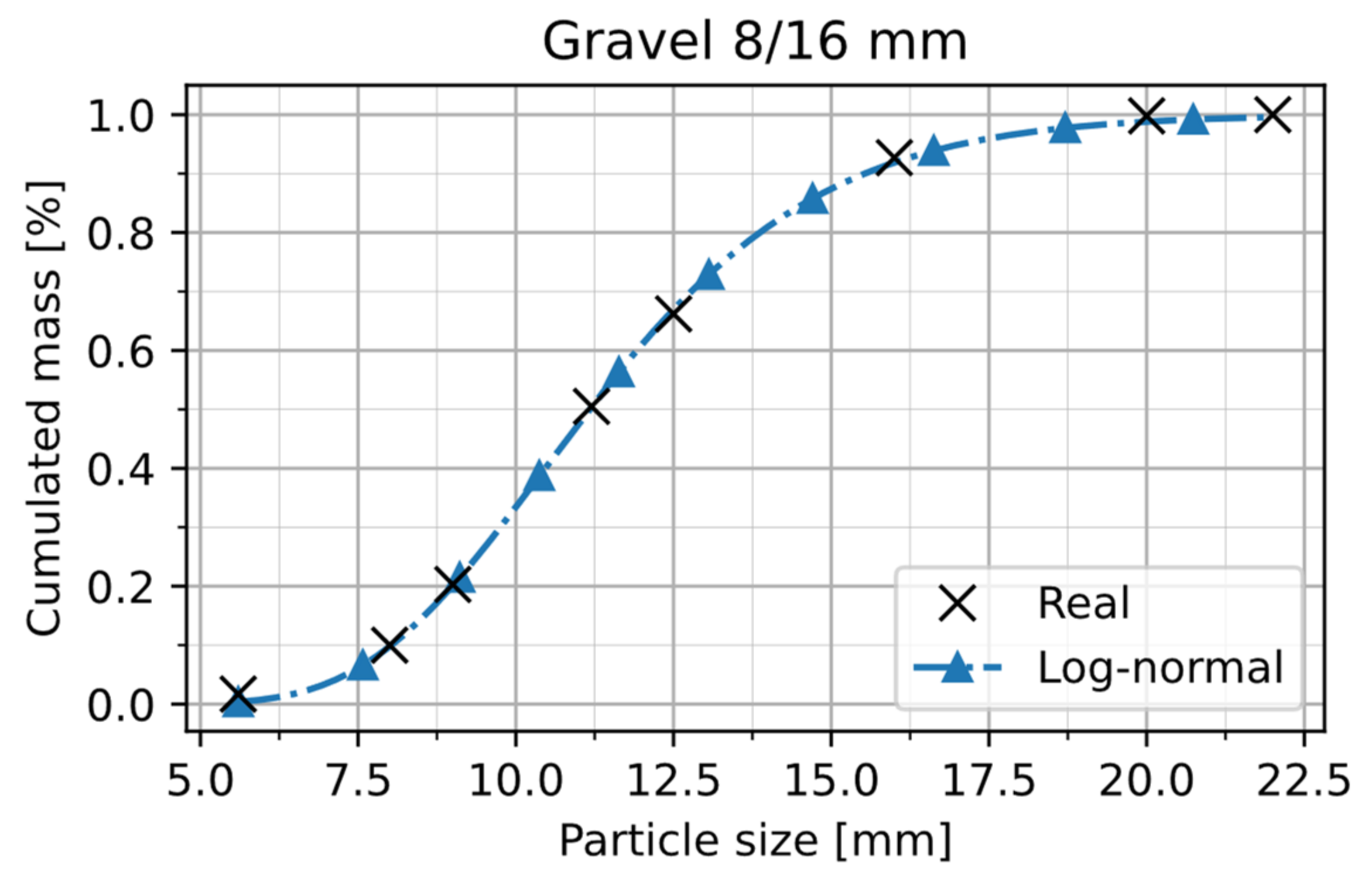
Next, the identified metamodels are used for the parameter identification in a MBGC process. For this, an unknown material—Gravel 8/16 mm—is used. Following the scheme, in Figure 2, first some experimental investigations on the real material have to be carried out to determine the particle size distribution of the material. Particle size distribution as well as the fitting of the Log-normal distribution are shown in Figure 16. The corresponding values for and as well as the target values for shear angle and bulk density are shown in Table 3. Furthermore, the table contains the value for determined by Jenike-wall-friction-tester.
The optimization method used for calibration is a L-BFGS algorithm (Limited-memory BFGS), which belongs to the family of quasi-Newton methods. For error calculation, the squared residuals for shear angle and bulk density are cumulated using Equation (11).
Due to the fact that there are 2 equations (Equations (9) and (10)) and 6 unknown parameters (), the system is underdetermined, which means there are several parameter combinations leading to the desired response values. In order to reduce the number of possible parameter combinations and identify a single solution, there are several possibilities. One would be the usage of other calibration experiments to produce more response values leading to more equations. Another possibility is to add some additional constraints. Constraints can be fixed values for some parameters as well as inequality constraints, e.g., . Here, we use fixed parameter values (Table 4). These values are based on previous investigations with the same bulk material done by Roessler et al. [17].
Using the constraints above, the optimization algorithm identified the parameter set shown in Table 5 to be optimal. The final optimization error was 1.034 × 10⁻¹¹. If the parameters from Table 3, Table 4 and Table 5 are entered into Equations (6) and (7), the estimated response values are and .
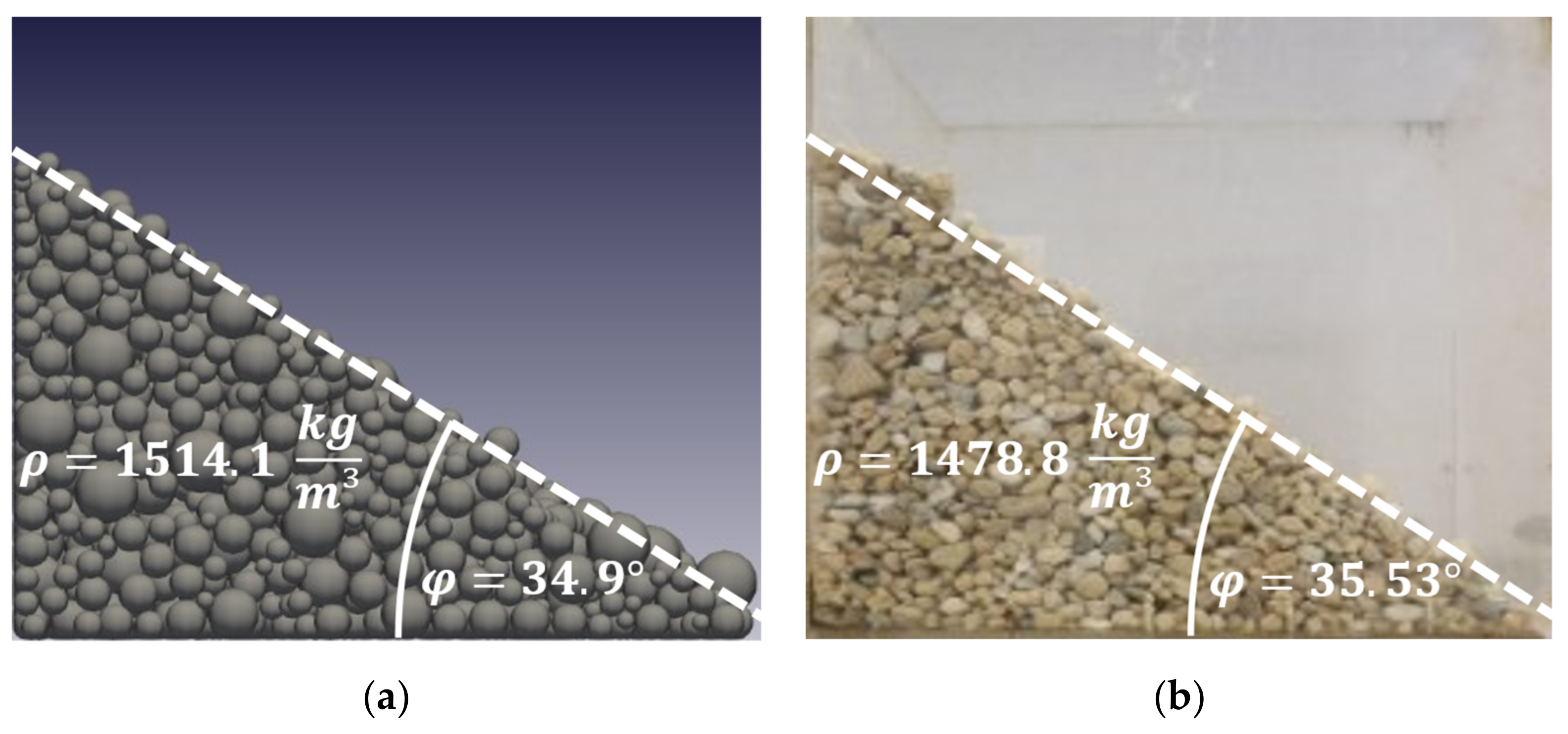
For validation, a simulation with the identified parameter values was done. The results show a very good agreement with the experimentally determined values. The simulated values are and . This corresponds to a relative error of 1.77% for the shear angle respectively 2.38% for bulk density. This almost corresponds to the stochastic fluctuation range of the measurements and can therefore be seen as very accurate. Figure 17 shows a comparison between the simulated and the real material behavior.
5. Discussion
The results above show that MBGC can be successfully used to identify a parameter set that provides the desired bulk material behavior. This can be seen as a proof of principle that the methodology works. In order to be able to make reliable statements on the performance and possible limitations of the methodology, further investigations are necessary regarding the calibration of other bulk materials, the metamodeling of new material domains (e.g., cohesive materials) as well as the variation and tuning of the different parts of the metamodeling process.
Furthermore, it could be proven that analytical equations exist which can be used to accurately model the relationships between the input and output parameters of a DEM simulation. Symbolic regression respectively genetic programming is an effective way to identify these equations. Although most of the points can be explained by the identified equations, there are also some outliers where the estimated value has a relatively high deviation from the real value.
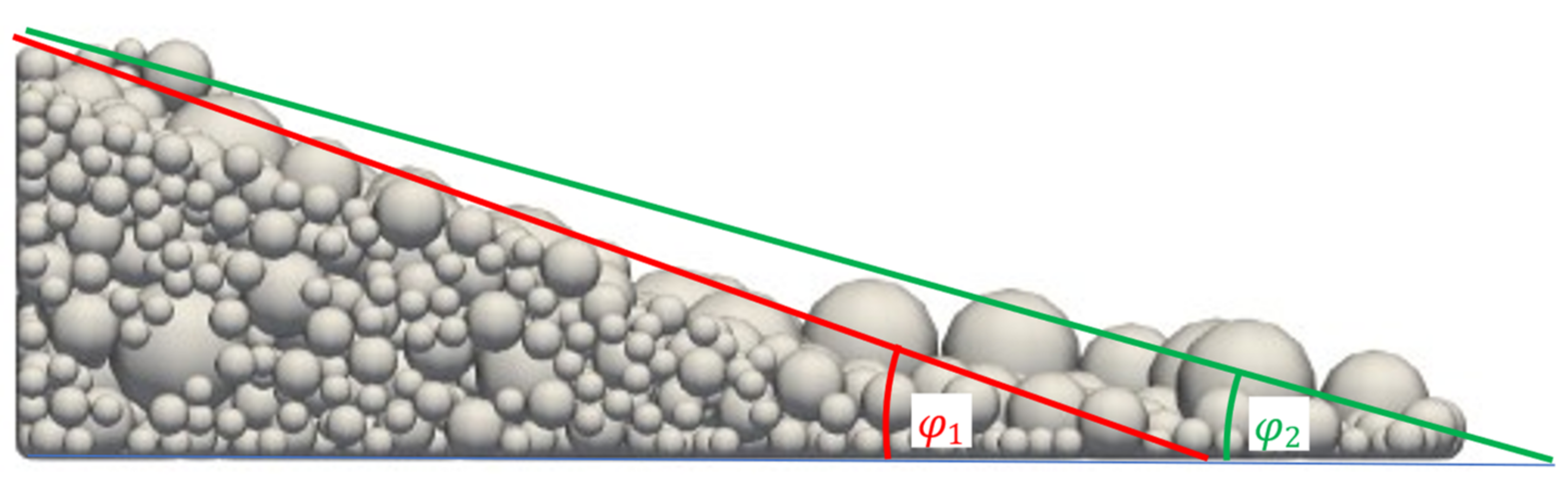
Outliers in shear angle estimation can be attributed to inadequacies in shear angle calculation. Shear angle calculation is based on the assumption that a flat flank is formed. The calculation of the angle is then done with help of linear regression. On closer inspection of the outliers, it was found that all of them had a curved flank leading to highly varying values in shear angle calculation (Figure 18). It is suspected that this uncertainty affecting the quality of the training and test data, which finally leads to the prediction errors. This means that in parameter space areas where these curved flanks occur, the metamodel has only limited validity.
The Problem of ambiguity of parameter combinations is still present, even with MBGC. A requirement to solve this problem is to have as many equations as unknown variables. Additional equations mean more response values. If there is not the possibility to extract or measure more response values as shown in the example above, some of the unknown parameters should be set to fixed.
Furthermore, the suitability of the identified parameter sets for simulating other mechanical behaviors of non-cohesive materials was not verified. Bulk density and shear angle characterize the flow behavior of the material. Accordingly, the identified parameter sets will lead to a realistic flow behavior in the simulations but not necessarily to realistic drag forces when, for example, soil-tool-interaction is simulated. For simulating other mechanical behaviors, other response variables must be included in the calibration.
6. Conclusions
In the present article, a new calibration method for the determination of material specific parameters in discrete element simulations has been introduced. Metamodel-based global calibration (MBGC) represents a paradigm shift in the field of DEM calibration, because it is the first method which does not include iterative DEM simulations in the calibration sequence. Instead, a global metamodel capable of estimating the behavior of different bulk materials in a predefined calibration experiment is used. Creating this metamodel is a one-time effort in contrast to classical calibration approach. Important factors in global meta-modelling are the sampling method as well as the kind of metamodel. Good space-filling properties of a sampling can be achieved by using the FSSF-f method. Symbolic regression respective genetic programming can be used to identify analytical equations which model the relationships between the input parameters and the result variables of a DEM simulation very well. Analytic equations are much better in terms of readability and human interpretability than, for example, matrix representations of weight factors or coefficients as used by other metamodels.
The identified equations can be used to calibrate a wide range of non-cohesive materials. As an application and validation example, the calibration of gravel 8/16 mm was shown. Future investigations will concentrate on generating new metamodels, e.g., for cohesive bulk materials as well as new calibration experiments. These experiments can be used to generate more response values and solve the problem of ambiguity of parameter sets without additional constraints. Another focus of future investigations will be the application of the methodology on complex-shaped particles. For this, superquadrics can be used to achieve a parametric description of the particle shape.
Author Contributions
Conceptualization, C.R.; methodology, C.R.; software, C.R.; validation, C.R.; formal analysis, C.R.; investigation, C.R.; data curation, C.R.; writing—original draft preparation, C.R.; writing—review and editing, F.W.; visualization, C.R.; supervision, F.W. All authors have read and agreed to the published version of the manuscript.
Funding
Open Access Funding by the Publication Fund of the TU Dresden.
Data Availability Statement
Not Applicable.
Conflicts of Interest
The authors declare no conflict of interest.
References
- Grima, A.; Wypych, P. Discrete element simulation of a conveyor impact-plate transfer: Calibration, validation and scale-up. Aust. Bulk Handl. Rev. 2010, 3, 64–72. [Google Scholar]
- Hess, G.; Richter, C.; Katterfeld, A. Simulation of the dynamic interaction between bulk material and heavy equipment: Calibration and validation. In Proceedings of the 12th International Conference on Bulk Materials Storage, Handling and Transportation, Darwin, Australia, 11–14 July 2016; pp. 427–436. [Google Scholar]
- Obermayr, M.; Vrettos, C. Anwendung der Diskrete-Elemente-Methode zur Vorhersage von Kräften bei der Bodenbearbeitung. Geotechnik 2013, 36, 231–242. [Google Scholar] [CrossRef]
- Tijskens, E.; Ramon, H.; Baerdemaeker, J. Discrete element modelling for process simulation in agriculture. First International ISMA Workshop on Noise and Vibration in Agricultural and Biological Engineering. J. Sound Vib. 2003, 3, 493–514. [Google Scholar] [CrossRef]
- Zhao, J.; Xiao, J.; Lee, M.L.; My, Y. Discrete element modeling of a mining-induced rock slide. SpringerPlus 2016, 5, 1633. [Google Scholar] [CrossRef] [PubMed] [Green Version]
- Kirsch, S. DEM Model Calibration for vertical filling: Selection of adequate trials and handling randomness. In Proceedings of the 15th Weimar Optimization and Stochastic Days (2018), Weimar, Germany, 21–22 June 2018. [Google Scholar]
- Kodam, M.; Curtis, J.; Hancock, B.; Wassgren, C. Discrete element method modeling of bi-convex pharmaceutical tablets: Contact detection algorithms and validation. Chem. Eng. Sci. 2012, 69, 587–601. [Google Scholar] [CrossRef]
- McKay, M.D.; Beckman, R.J.; Conover, W.J. A comparison of three methods for selecting values of input variables in the analysis of output from a computer code. Technometrics 1979, 21, 239–245. [Google Scholar] [CrossRef]
- Do, H.Q.; Aragon, A.M.; Schott, D.L. A calibration framework for discrete element model parameters using genetic algorithms. Adv. Powder Technol. 2018, 29, 1393–1403. [Google Scholar] [CrossRef]
- Richter, C.; Roessler, T.; Kunze, G.; Katterfeld, A.; Will, F. Development of a standard calibration procedure for the DEM parameters of cohesionless bulk materials—Part II: Efficient optimization-based calibration. Powder Technol. 2020, 360, 967–976. [Google Scholar] [CrossRef]
- Rackl, M.; Hanley, K.J. A methodical calibration procedure for discrete element models. Powder Technol. 2017, 307, 73–83. [Google Scholar] [CrossRef] [Green Version]
- Benvenuti, L.; Kloss, C.; Pirker, S. Identification of dem simulation parameters by artificial neural networks and bulk experiments. Powder Technol. 2016, 291, 456–465. [Google Scholar] [CrossRef]
- Barton, R.R. Simulation optimization using metamodels. In Proceedings of the 2009 Winter Simulation Conference (WSC), Austin, TX, USA, 13–16 December 2009; pp. 230–238. [Google Scholar] [CrossRef] [Green Version]
- Regis, R.G. Stochastic radial basis function algorithms for large-scale optimization involving expensive black-box objective and constraint functions. Comput. Oper. Res. 2011, 38, 837–853. [Google Scholar] [CrossRef]
- Crombecq, K.; Learmans, E.; Dhaene, T. Efficient space-filling and non-collapsing sequential design strategies for simulation based modeling. Eur. J. Oper. Res. 2011, 214, 683–696. [Google Scholar] [CrossRef] [Green Version]
- Wensrich, C.M.; Katterfeld, A. Rolling friction as a technique for modelling particle shape in DEM. Powder Technol. 2012, 217, 409–417. [Google Scholar] [CrossRef]
- Kloss, C.; Goniva, C.; Hager, A.; Amberger, S.; Pirker, S. Models, algorithms and validation for opensource DEM and CFD-DEM. Prog. Comput. Fluid Dyn. 2012, 12, 140–152. [Google Scholar] [CrossRef]
- Roessler, T.; Richter, C.; Katterfeld, A.; Will, F. Development of a standard calibration procedure for the DEM parameters of cohesionless bulk materials—Part I: Solving the problem of ambiguous parameter combinations. Powder Technol. 2019, 343, 803–812. [Google Scholar] [CrossRef]
- Thornton, C. Numerical simulations of deviatoric shear deformation of granular media. Géotechnique 2000, 50, 43–53. [Google Scholar] [CrossRef]
- Li, Y.; Xu, Y.; Thornton, C. A comparison of discrete element simulations and experiments for “sandpiles” composed of spherical particles. Powder Technol. 2005, 160, 219–228. [Google Scholar] [CrossRef]
- Boac, J.M.; Casada, M.E.; Maghirang, R.G.; Harner, J.P. 3-D and quasi-2-D discrete element modeling of grain commingling in a bucket elevator boot system. Trans. ASABE 2012, 55, 659–672. [Google Scholar] [CrossRef]
- Liu, H.; Ong, Y.-S.; Cai, J. A survey of adaptive sampling for global metamodeling in support of simulation-based complex engineering design. Struct. Multidiscip. Optim. 2018, 57, 393–416. [Google Scholar] [CrossRef]
- Fuhg, J.N.; Fau, A.; Nackenhorst, U. State-of-the-art and comparative review of adaptive sampling methods for kriging. Arch. Comput. Methods Eng. 2021, 28, 2689–2747. [Google Scholar] [CrossRef]
- Halton, J.H. On the efficiency of certain quasi-random sequences of points in evaluating multi-dimensional integrals. Numer. Math. 1960, 2, 84–90. [Google Scholar] [CrossRef]
- Sobol, I.M. On the distribution of points in a cube and the approximate evaluation of integrals. USSR Comput. Math. Math. Phys. 1967, 7, 86–112. [Google Scholar] [CrossRef]
- Shang, B.; Apley, D.W. Fully-sequential space-filling design algorithms for computer experiments. J. Qual. Technol. 2020, 53, 173–196. [Google Scholar] [CrossRef]
- Gunzburger, M.; Burkardt, J. Uniformity Measures for Point Sample in Hypercubes. 2004. Available online: https://people.sc.fsu.edu/~jburkardt/publications/gb_2004.pdf (accessed on 4 August 2021).
- Worm, T.; Chiu, K. Prioritized grammar enumeration: Symbolic regression by dynamic programming. In Proceedings of the 15th Annual Conference on Genetic and Evolutionary Computation GECCO’13, Amsterdam, The Netherlands, 6–10 July 2013; pp. 1021–1028. [Google Scholar] [CrossRef]
- Petersen, B.K.; Larma, M.L.; Mundhenk, T.N.; Santiago, C.P.; Kim, S.K.; Kim, J.T. Deep symbolic regression: Recovering mathematical expressions from data via risk-seeking policy gradients. In Proceedings of the International Conference on Learning Representations, Vienna, Austria, 3–7 May 2021. LLNL-CONF-790457. [Google Scholar]
- Trevor, S. GPLearn. 2021. Available online: https://gplearn.readthedocs.io/en/stable/index.html (accessed on 4 August 2021).
Figure 1.
Scheme of a classic calibration approach for discrete element method.

Figure 2.
Scheme of metamodel-based global calibration (MBGC).

Figure 3.
Granular materials considered to quantify the boundaries of the investigated material domain: (a) coke; (b) stone chippings 2-5 mm; (c) limestone; (d) gravel 2/8 mm; (e) gravel 16/32 mm; (f) dry sand; (g) woodchips; (h) dry corn.
Figure 3.
Granular materials considered to quantify the boundaries of the investigated material domain: (a) coke; (b) stone chippings 2-5 mm; (c) limestone; (d) gravel 2/8 mm; (e) gravel 16/32 mm; (f) dry sand; (g) woodchips; (h) dry corn.

Figure 4.
Comparison how good different analytical distributions functions fit the real particle size distribution of the example materials.
Figure 4.
Comparison how good different analytical distributions functions fit the real particle size distribution of the example materials.

Figure 5.
Structure of the shear box test: (left) initial state before opening the flap; (right) final state.
Figure 5.
Structure of the shear box test: (left) initial state before opening the flap; (right) final state.

Figure 6.
Alternative sequential sampling design strategies (initial samples in black dots, sequentially added samples in red squares): (a) space-filling sampling; (b) adaptive sampling [23].
Figure 6.
Alternative sequential sampling design strategies (initial samples in black dots, sequentially added samples in red squares): (a) space-filling sampling; (b) adaptive sampling [23].

Figure 7.
Benchmark of different sequential space-filling methods for 2-dimensional space. Blue bars show the mean value of 10 different designs. Black whiskers show the minimum and maximum values. (a) minimum intersite distance; (b) cover measure.
Figure 7.
Benchmark of different sequential space-filling methods for 2-dimensional space. Blue bars show the mean value of 10 different designs. Black whiskers show the minimum and maximum values. (a) minimum intersite distance; (b) cover measure.

Figure 8.
Benchmark of different sequential space-filling methods for 10-dimensional space. Blue bars show the mean value of 10 different designs. Black whiskers show the minimum and maximum values. (a) minimum intersite distance; (b) cover measure.
Figure 8.
Benchmark of different sequential space-filling methods for 10-dimensional space. Blue bars show the mean value of 10 different designs. Black whiskers show the minimum and maximum values. (a) minimum intersite distance; (b) cover measure.

Figure 9.
Representation of a function as an expression tree.

Figure 10.
Crossover.

Figure 11.
Point mutation.

Figure 12.
Subtree mutation.

Figure 13.
Hoist mutation.

Figure 14.
Residual Histogram for shear angle estimation.

Figure 15.
Residual histogram for bulk density estimation.

Figure 16.
Particle size distribution of Gravel 8/16 and fitting of Log-normal distribution.

Figure 17.
Validation of the identified set of parameters. (a) Simulated bulk material; (b) real bulk material.
Figure 17.
Validation of the identified set of parameters. (a) Simulated bulk material; (b) real bulk material.

Figure 18.
Varying values in shear angle calculation for curved flanks.


Table 1.
Coefficient of determination and mean squared error of analytical distribution functions.
| Metric | Mean Over All Materials | ||
|---|---|---|---|
| GGS | RRSB | LOGN | |
| Coefficient of determination | 0.8155 | 0.9925 | 0.9935 |
| Mean squared error | 0.0308 | 0.0012 | 0.0010 |
Table 2.
Parameter ranges used for data generation. The ranges define the parameter space in which the metamodel is valid.
Table 2.
Parameter ranges used for data generation. The ranges define the parameter space in which the metamodel is valid.
| Parameter | Symbol | Unit | Range |
|---|---|---|---|
| Young’s modulus of particles | 5 × 10⁶ … 5 × 10⁸ | ||
| Young’s modulus of walls | 5 × 10⁶ … 5 × 10⁸ | ||
| Poisson ratio for particles | - | 0.1 … 0.5 | |
| Coefficient of restitution particle-particle | - | 0.05 … 0.95 | |
| Coefficient of restitution particle-wall | - | 0.05 … 0.95 | |
| Coefficient of friction particle-particle | - | 0.0 … 1.0 | |
| Coefficient of friction particle-wall | - | 0.0 … 1.0 | |
| Coefficient of rolling friction particle-particle | - | 0.0 … 1.0 | |
| Coefficient of rolling friction particle-wall | - | 0.0 … 1.0 | |
| Particle density | 250 … 3000 | ||
| Median diameter of PSD | 0.40 … 25.6 | ||
| Standard Deviation of PSD | 0.07 … 1.17 |
Table 3.
Values of Gravel 8/16 determined in experimental investigations.
| Parameter/Response Value | Symbol | Unit | Value |
|---|---|---|---|
| Median diameter of PSD | mm | 11.16 | |
| Standard Deviation of PSD | mm | 0.26 | |
| Coefficient of friction particle-wall | - | 0.363 | |
| Shear angle | ° | 35.53 | |
| Bulk density | kg/m³ | 1478.8 |
Table 4.
Constraints introduced to reduce the number of possible solutions.
| Constraint |
|---|
Table 5.
Optimal parameter set identified by MBGC.
| Parameter | Value |
|---|---|
| 0.1852 | |
| 2608.4 |
Publisher’s Note: MDPI stays neutral with regard to jurisdictional claims in published maps and institutional affiliations. |
© 2021 by the authors. Licensee MDPI, Basel, Switzerland. This article is an open access article distributed under the terms and conditions of the Creative Commons Attribution (CC BY) license (https://creativecommons.org/licenses/by/4.0/).
Share and Cite
MDPI and ACS Style
Richter, C.; Will, F. Introducing Metamodel-Based Global Calibration of Material-Specific Simulation Parameters for Discrete Element Method. Minerals 2021, 11, 848. https://doi.org/10.3390/min11080848
AMA Style
Richter C, Will F. Introducing Metamodel-Based Global Calibration of Material-Specific Simulation Parameters for Discrete Element Method. Minerals. 2021; 11(8):848. https://doi.org/10.3390/min11080848
Chicago/Turabian StyleRichter, Christian, and Frank Will. 2021. "Introducing Metamodel-Based Global Calibration of Material-Specific Simulation Parameters for Discrete Element Method" Minerals 11, no. 8: 848. https://doi.org/10.3390/min11080848
Note that from the first issue of 2016, this journal uses article numbers instead of page numbers. See further details here.