
An Evolutionary Computation Approach for Twitter Bot Detection


1
Department of Engineering and Architecture, University of Trieste, 34127 Trieste, Italy
2
Department of Mathematics and Geosciences, University of Trieste, 34127 Trieste, Italy
*
Author to whom correspondence should be addressed.
Appl. Sci. 2022, 12(12), 5915; https://doi.org/10.3390/app12125915
Submission received: 18 May 2022
/
Revised: 6 June 2022
/
Accepted: 7 June 2022
/
Published: 10 June 2022
(This article belongs to the Special Issue Genetic Programming, Theory, Methods and Applications)
Abstract
:Featured Application
Our proposed application can be used to detect bot accounts on the social platform Twitter. Our models are based on evolutionary computation techniques such as genetic algorithms and genetic programming methods. These strategies enabled us to discover models with high interpretability of predictions and good generalization capabilities on unseen data as well.
Abstract
Bot accounts are automated software programs that act as legitimate human profiles on social networks. Identifying these kinds of accounts is a challenging problem due to the high variety and heterogeneity that bot accounts exhibit. In this work, we use genetic algorithms and genetic programming to discover interpretable classification models for Twitter bot detection with competitive qualitative performance, high scalability, and good generalization capabilities. Specifically, we use a genetic programming method with a set of primitives that involves simple mathematical operators. This enables us to discover a human-readable detection algorithm that exhibits a detection accuracy close to the top state-of-the-art methods on the TwiBot-20 dataset while providing predictions that can be interpreted, and whose uncertainty can be easily measured. To the best of our knowledge, this work is the first attempt at adopting evolutionary computation techniques for detecting bot profiles on social media platforms.
1. Introduction
Bot accounts in social network platforms and web applications represent a major threat to cybersecurity scenarios since their presence could harm user experience in various ways, such as bad advertisements, spam links, phishing, and fake content. Moreover, bot accounts that are part of botnets can harm the scalability of social networks by leveraging distributed denial of service (DDoS) attacks that can slow down hosting networks, causing massive interruptions of the services that these applications aim to offer [1,2,3,4].
Twitter is one of the social platforms that are mostly targeted by bot developers due to its large political and social impact, and the high number of users that sign into it every day. Bot accounts are also exploited to sway political opinions during political campaigns. Furthermore, developers usually take advantage of their bots to badly influence the audience’s opinion about several kinds of hot topics. To this end, several research works have been developed, aiming at discovering effective models that can detect whether a given user profile is authentic or not. However, correctly detecting every type of bot account is extremely challenging given the high heterogeneity and the variety that bot profiles exhibit in terms of behavior and final goals. For these reasons, new approaches to the problem are considered to be of high relevance [5], since they may help to define a method that can generalize among different types of bot accounts while effectively detecting most of them.
In this paper, we focus our research efforts on detecting bot accounts that are active on Twitter. In particular, we propose a novel approach for Twitter bot detection that leverages evolutionary computation strategies such as genetic algorithms and genetic programming. We show that genetic programming can be employed to learn a model in the form of a formula that can achieve competitive detection accuracy while being arguably more interpretable than other machine learning (ML) models available in the literature, which are based on complex, often black-box, architectures. Moreover, we leverage genetic algorithms to learn the weights of a neural network with no hidden layers and a single output perceptron in an evolutionary fashion. We evaluate our model using the TwiBot-20 dataset that was created as a reference benchmark dataset for this specific task by Feng et al. [6], and we show that our classification models can achieve qualitative performance close to the top state-of-the-art methods. Furthermore, our classification models can provide predictions that can be interpreted and whose uncertainty can be easily measured by inspecting the models themselves and checking the components that contribute the most to detection. In this way, we provide a valid alternative to black-box models, which can achieve slightly higher detection accuracy at the cost of learning extremely complex models whose predictions cannot be justified.
The main contributions we make through this work can be summarized as follows:
- (i)
- describing and analyzing the main features that can be associated with user accounts on Twitter to understand the types of property that may help to discriminate between human profiles and bot profiles;
- (ii)
- proposing a novel approach based on genetic algorithms and genetic programming to detect bot profiles on Twitter, and presenting two classification models that exhibit good qualitative performance and generalization capabilities, while ensuring interpretability of predictions;
- (iii)
- providing a way to compute how much our models are confident with a given prediction.
Thus, in this work we try to give an answer to the following research questions:
- RQ1: is it possible to obtain interpretable models with good generalization capabilities for Twitter bot detection?
- RQ2: can we trust predictions of ML models based on Twitter bot detection?
The paper is structured as follows. Section 2 describes what are some related works and their limitations. Section 3 presents the choice of the dataset, a brief analysis of the data, and the preprocessing steps taken. In Section 4 we describe how genetic algorithms and genetic programming are used for the classification of Twitter bots, while Section 5 contains the comparison of the proposed models with the results in the literature. Section 6 provides a final overview of the results obtained and how to answer the research questions. Finally, Section 7 provides a summary of the contributions of the paper and some directions for future research.
2. Related Work
In this section, we briefly discuss the most effective spam and bot detection methods that have already been proposed in the literature. The early works were based on the detection and filtering of spam links from URLs, messages, and web pages. Becchetti et al. [7] combined several metrics such as degree correlations, number of neighbors, and TrustRank [8] to build web spam classifiers. Thomas et al. [9] presented a real-time system named ”Monarch” that crawls URLs as they are submitted to web services, and determines whether the URLs direct to spam websites. Benczúr et al. [10] built spam classifiers that take advantage of the similarity between spam pages to detect whether an unknown website is spam or legitimate. Bratko et al. [11] investigated an approach based on adaptive statistical data compression models for spam filtering.
Looking at more recent works, Grier et al. [12] presented a detailed analysis of spam on Twitter to demonstrate the ineffectiveness of blacklists and found that 8% of 25 million URLs point to phishing, malware, and scams listed on popular blacklists, while, on average, more than 90% of visitors view a page before it becomes blacklisted. Gao et al. [13] proposed an online spam filtering system that reconstructs spam messages into campaigns for spam classification. Jindal et al. [14] studied the opinion spam and trustworthiness of online opinions in the context of product reviews and implemented a logistic regression classifier to detect spam in these kinds of data. Ott et al. [15] studied deceptive opinion spam and developed a support vector machine (SVM) and a naive Bayes classifier to detect spam. Lee et al. [16] proposed “WarningBird”, a near real-time detection system for suspicious URLs in Twitter streams that investigates correlations of URL redirect chains extracted from texts of tweets. While most of the aforementioned methods are focused on detecting spam on general messages and web pages, a good percentage of the most recent works are focused on Twitter bot detection. However, general spam detection methods are still largely explored in the recent literature and their results continuously inspire the study and development of novel bot detection strategies.
Many research works investigated how to use text from tweets and meta-data to perform bot detection. Chu et al. [17] proposed a classification algorithm consisting of an entropy-based component, a spam detection component, an account properties component, and a decision maker to assess whether a given account is a bot or a human. Perdana et al. [18] proposed a bot detection model based on time interval entropy and tweet similarity, where the former was calculated using timestamp collection, while the latter was calculated using uni-gram matching-based similarity. Cresci et al. [19] analyzed online users’ activities and extracted them from the sets of DNA-inspired strings encoding users’ actions. Subsequently, they applied DNA-based analysis methods to detect spam bot profiles. Beskow et al. [20] leveraged random string detection applied to user screen names to filter bot accounts on Twitter. Ahmed et al. [21] presented a set of 14 generic statistical features to identify spam profiles on online social networks (OSNs). Despite most approaches being based on supervised methods, there also exist models that are totally unsupervised. For instance, many works are based on studying how to perform bot and spam classification by analyzing anomalous and suspicious behavior of social profiles. Chavoshi et al. [22] developed a system named “DeBot” that consists of a novel lag-sensitive hashing technique that clusters user accounts into correlated sets in near real time. They leveraged cross-user features and activity correlation to detect bots without using labeled data. Miller et al. [23] approached the bot detection problem on Twitter as an anomaly detection problem, where they used 95 one-gram features extracted from the text of the tweets along with user metadata information. They discriminated between spam bot profiles and genuine users using two modified versions of the stream clustering algorithms, StreamKM++ [24] and DenStream [25], treating outliers as spammers. Wang [26] proposed a directed social graph model encoding follow relationships and used a Bayesian classifier to discriminate between normal and anomalous behavior. Stringhini et al. [27] collected data about spamming activity to create a large dataset and analyzed anomalous behavior to detect spammers in social networks. Cao et al. [28] implemented a malicious account detection system called “SynchroTrap” that clusters user accounts according to the similarity of their actions and analyzes anomalous and suspicious actions to cluster malicious accounts together. Several works are also based on analyzing the behavior of spammers on Twitter to discover the best strategies to detect them. Yardi et al. [29] showed the existence of structural network differences between spam accounts and genuine user accounts. Ghosh et al. [30] investigated link farming in the Twitter network and found that a majority of spammers’ links are farmed from a small fraction of Twitter users called “social capitalists”. Additionally, they proposed a user ranking scheme that penalizes users for connecting to spammers.
Recent Twitter bot detection and spam detection models are mainly based on training machine learning models and deep neural networks after the implementation of proper feature selection and feature engineering phases. These methods take advantage of user metadata information (e.g., number of followers and number of tweets), and semantic information that can be extracted from a sample of user’s tweets (e.g., the minimum time interval between two consecutive tweets, the number of URLs). Ferrara et al. [31] analyzed disinformation campaigns conducted by means of bot profiles during the 2017 French presidential election and took advantage of a mixture of ML models and cognitive behavioral modeling techniques to discriminate between humans and bots on social networks. Furthermore, they [32] discussed the characteristics of modern social bots and how features related to the content, network, sentiment, and temporal patterns of activity can help discriminate between humans and bots. Yang et al. [33] investigated the most common evasion techniques used by Twitter spammers and designed several detection features that can be leveraged to build ML models for Twitter spammer detection. The top-performing machine learning models for Twitter bot detection available in the current literature are based on random forest classifiers applied to hand-made features derived from meta-data properties and semantic properties. Benevenuto et al. [34] collected a large dataset of Twitter with more than 54 milion of users, 1.9 billion links, and almost 1.8 billion tweets. They adopted this dataset to train an SVM model running fivefold cross validation. McCord et al. [35] crawled using Twitter API a set of active users and built several classification models using user-based and content-based features that should be different between spammers and genuine profiles. Their results showed that the random forest classifier is the most effective model. Yang et al. [36] built a rich collection of labeled datasets to train random forest classifiers based on user metadata and additional hand-made features. Lee et al. [37] presented a long-term study of social honeypots for detecting spam bot profiles and content polluters on social platforms and trained random forest classifiers with different sets of hand-made features generated using metadata information. The Botometer [38] is a publicly available service that takes advantage of more than 1000 features to identify Twitter bot accounts on demand using seven different random forest classifiers.
Recent literature also includes several works based on deep neural networks that leverage meta-data and text information to discriminate between spammers, bots, and humans. Alsaleh et al. [39] implemented a browser plug-in called “Twitter Sybils Detector” (TSD) that leverages a feed-forward neural network with a set of hand-made features to detect fake accounts on Twitter. Ren et al. [40] implemented a neural network model to learn document-level representation for detecting deceptive opinion spam, where sentence representations are learned using a convolutional neural network (CNN), and combined using a gated recurrent neural network. Lai et al. [41] implemented a recurrent convolutional neural network for text classification to learn contextual information of words, and Zhang et al. [42] extended this work using a recurrent convolutional neural network (DRI-RCNN) to identify misleading reviews using word contexts and deep learning. Alhosseini et al. [43] implemented a graph convolutional neural network (GCNN) to detect spam bot profiles using a set of metadata features along with low-dimensional representations (that is, node embeddings) of the social graph that can be derived from social relationships of user accounts. Kudugunta et al. [44] proposed the adoption of a deep neural network based on a contextual long short-term memory architecture that can jointly leverage user metadata and semantic information to detect whether a given tweet has been written by a bot account or not. Wei et al. [45] adopted recurrent neural networks based on bidirectional long short-term memory with word embeddings to capture features across tweets and detect bot accounts. Besides recurrent neural networks and convolutional neural networks, attention has also been reserved for generative adversarial networks (GANs). Li et al. [46] proposed “CS-GAN”, a model that combines reinforcement learning, generative adversarial networks, and recurrent neural networks to generate category sentences. Stanton et al. [47] implemented a generative adversarial network that uses a limited set of labeled data to detect spam in online posts.
3. Data Preparation
There are various datasets that are publicly available on the Internet and that can be adopted for Twitter bot detection task [36,37,48,49,50,51]. Apart from TwiBot-20, midterm-18 is the largest dataset containing Twitter bots. The drawback is that it is focused on a political-related domain and it does not provide data that can be associated with users involved in more general topics. Most of the available datasets provide only property (user account attributes) information while missing semantic (tweets posted) and neighbor (followers and followings) information. Therefore, low user diversity, data scarcity, and limited user information are the main problems encountered in the aforementioned datasets. For these reasons, to build our detection models, we decided to adopt the TwiBot-20 dataset, which was kindly granted to us by its authors Feng et al. [6]. TwiBot-20 is currently the only dataset that provides property, semantic, and neighbor information at the same time. Specifically, it includes 229,573 users (human and bot accounts), 8,723,736 properties, 33,488,192 tweets, and 455,958 neighbors, and it is by far the largest available dataset for Twitter bot detection. Additionally, it contains user accounts related to a variety of domains (politics, business, entertainment, and sport) and located in various geographical locations, in contrast to other available datasets that focus on collecting information for specific topics and that are limited in size. The dataset of Feng et al. [6] was used as a benchmark for the state-of-the-art methods and therefore it probably represents the best choice for building and evaluating novel detection algorithms as a result of the high number of baselines that it offers. Furthermore, as stated in the aforementioned paper, TwiBot-20 is much more challenging than other available datasets, and this allows the building of more robust models. State-of-the-art methods fail to achieve extremely high performance when trained and evaluated on TwiBot-20, therefore, this dataset may help to define models with better generalization capabilities.
3.1. Data Description
TwiBot-20 stores information in JSON format and consists of four files: train.json, dev.json, test.json, and support.json. Each file contains an array of JSON objects where each JSON object is a user account with a set of properties including user ID, name, screen name, domain, followings, followers, tweets, and a label indicating whether the user is human (0) or bot (1). TwiBot-20 was collected from July 2020 to September 2020. Properties and semantic information were retrieved using Twitter API and a sample of 200 tweets, on average, was retrieved for each user along with properties available from Twitter API calls, while approximately 20 neighbors’ IDs were collected by following user relationships (10 followers and 10 followings). Regarding the data annotation strategy adopted during the generation of the TwiBot-20 dataset, the characteristics of labeling bot profiles that were taken into account during this step can be summarized as follows: API usage, lack of originality and variety in published tweets, identical tweets repeated multiple times, and massive usage of URLs in the posts. The authors decided to partition the labeled users dataset, consisting of 11,826 user profiles, with a 7:2:1 random partition that generated, respectively, a training set (train.json), validation set (dev.json), and test set (test.json). The authors also provided unsupervised users with a support set (support.json) to preserve the dense graph structure and follow relationship forms. We adopt the training set to drive the evolutionary process of the proposed techniques, the validation set to choose the best model according to the generalization error, and the test set to evaluate the model. As we can see from Figure 1, each set is balanced with respect to the target class, with bot accounts that are a little more represented.
3.2. Feature Extraction
As we mentioned before, the TwiBot-20 dataset comes with both user metadata information and tweets content information. For this reason, we extract a set of meaningful features from the available data to build a dataset where each user profile can be represented as a fixed-sized vector of real-number values. This step consists of a data preparation process in which feature engineering and feature selection are performed to map each user profile contained in the original dataset into a space contained in where . Hence, this preliminary step is executed for each user account independently. The most meaningful metadata properties associated with user accounts can be retrieved by Twitter API calls (Twitter API docs for user profile. https://developer.twitter.com/en/docs/twitter-api/v1/data-dictionary/object-model/user, accessed on 16 December 2021). We describe these properties as follows.
- id: unique numerical identifier of the user account;
- screen_name: unique string composed of letters, digits, and underscores, which identifies the username of the Twitter account;
- name: name visualized for the user account;
- description: optional field indicating the description visualized for the user account;
- URL: optional field indicating an URL for the user account;
- location: optional attribute indicating a location for the user account;
- created_at: timestamp indicating the user account creation time;
- statuses_count: total number of tweets (including retweets) published by the user during the entire account lifetime;
- followers_count: total number of followers of the user account;
- friends_count: total number of followings of the user account;
- favourites_count: total number of posts that the user has marked as favorites;
- listed_count: total number of public lists that the user is a member of.
Additionally, TwiBot-20 provides us with a sample of approximately 200 tweets for each user account (each tweet is a text string), where these tweets correspond to the latest published tweets for a given user account, and thus they are the most representative of the behavior of that user on Twitter during the period in which the data has been collected. For this reason, we believe that deriving features from tweets that can be joined with user metadata information would lead to a significant improvement in the predictive power of an ML model for bot detection. As a first step, we employ natural language processing techniques to properly preprocess users’ tweets while converting them from strings to lists of tokens. In particular, we perform the following operations for each tweet of a given user account using the NLTK (NLTK Library. https://www.nltk.org/, accessed on 4 January 2022) library in Python 3.8:
- we first perform lowering of text and trimming. Then, we extract the hashtags and the mentioned users that are eventually contained in the current tweet. We also count the number of URLs and we check whether the tweet is an authentic published tweet or a retweet;
- we perform tokenization of the text using a Tweet Tokenizer, and part-of-speech tagging after proper punctuation, URLs, and digits removal;
- we use a Word Net Lemmatizer to lemmatize the tagged tokens of the previous step in this pipeline;
- we filter lemmatized tokens by excluding stop words and single-character words;
- we return the list of tokenized tweets obtained by following this pipeline.
Once this pipeline is run, we obtain for each user profile in TwiBot-20 a list of tokenized tweets, where each of these consists of a list of tokens that eventually includes hashtags and mentioned users. Moreover, we decide to divide each of these lists of tweets into two sub-lists, one containing only tweets that have been directly published by the user and one containing only the retweets. The main reason for this choice can be attributed to the fact that published tweets are probably more interesting for doing a meaningful analysis of word frequency. This expedient may enable an ML model to determine information related to the writing behavior of a given user. Including retweets in this kind of analysis would probably lead to misleading conclusions. However, it is also worth investigating the frequency of retweets compared to the frequency of authentic tweets. From now on, we are referring to the list of tweets as the list of published tweets that are not retweets, if not differently specified. By using user metadata along with tokenized tweets and retweets, it is possible to derive additional properties that can be adopted as hand-made features in the training phases of ML models. The set of features that we derive for each user account independently starting from user metadata, tweets, and retweets, are presented as follows.
- Statistical measures over tweet lengths: a set of characteristics derived by applying statistical measures, namely, mean, median, maximum minimum range, and standard deviation, to an array containing the lengths, in terms of the number of characters, of the original tweets. In particular, the standard deviation of the lengths of tweets enables us to say whether the user tends to publish tweets of approximately the same length (e.g, identical tweets, which are common among certain types of bot accounts) or tends to vary a lot the size of the published posts. Figure 2 shows that bot profiles are more likely to exhibit a lower standard deviation of tweet lengths than humans, which means that bot profiles are more likely to publish tweets with approximately the same length and presumably the same type of content;
- Frequency over the content of collected tweets and retweets: a set of features that measure the frequency of appearances of retweets, URLs, mentioned users, and hashtags, over the sample of tweets and retweets retrieved via Twitter API for a given user account u. Each feature of this category is computed using the following formula:where , , , is the set of tokenized tweets for user u and is the set of tokenized retweets for user u while is a function that counts the number of times a word of category c appears in the input list of tokenized posts (tweets and retweets), including duplicates. Therefore, we are describing the mean number of hashtags, mentioned users, and URLs, for each retrieved tweet and retweet. Similarly, the frequency of retweets is calculated as follows.One intuitive reason that may justify the derivation of features such as, for example, the frequency of retweets and URLs, can be explained by observing the general trend of a significant percentage of bot profiles that avoid publishing self-made tweets and prefer to retweet specific content several times and post several URLs that usually redirect to spam, phishing, or, in general, undesirable web pages. Moreover, several bot profiles that, for example, promote political campaigns, are used to expose a high frequency of mentioned users, since they usually include the target politician’s screen name in their tweets. Figure 3 confirms that bot profiles are more likely to exhibit a higher frequency of retweets than humans. Additionally, the frequency of words used to write tweets by a given user u is calculated as follows:In this way, we are describing the mean number of words (tokens that are not hashtags nor mentioned users) for each published tweet, including duplicates. Since this measure should account for the writing behavior of user u, we decide to exclude from the computation of this property the words contained in retweets, which are tweets that have not been written by u and thus they present a potentially different writing behavior;
- Statistical measures over raw counts: set of features derived by applying statistical measures, namely, mean, median, max, min, and standard deviation, to three arrays containing, respectively, the raw counts of the distinct words, hashtags, and mentioned users. Raw counts can be extracted from tokenized published tweets set and tokenized retweets set of a given user u. These measures are computed considering distinct hashtags and mentioned users that appear in both tweets and retweets of user u. We consider distinct words that appear only in published tweets at least three times, and thus when computing these statistical measures on the raw counts of distinct words, we exclude words that appear in retweets of user u. As a matter of fact, these types of measures over raw word counts aim to capture the writing behavior of a given user u. Quite to the contrary, when computing these statistical measures over the raw counts of hashtags and mentioned users, we consider those that are contained in retweets and tweets as well, since it can be arguably verified that a hashtag or a mentioned user that appears in a retweet of user u gains additional exposure even though the user u has posted it through a retweet. These measures can be useful because they can estimate, for example, how the frequency of words varies within the sample of tweets collected for the user u. In particular, a low standard deviation of raw word counts is expected if user u has a uniform behavior when writing posts. In contrast, this value is high if few words are over-used, while many others are less sponsored. For these reasons, these types of measures can help to discriminate between bot profiles and human profiles by analyzing their writing behavior;
- Reputation: this feature is computed by analyzing the number of followers of a given user u compared to the number of followings, or friends, of the same user:This property exhibits a high value when the user u has a large number of followers and a few followings, such as celebrities and politicians. Quite the opposite, bot accounts that usually have a large number of followings and a few followers are likely to exhibit a low reputation value. Figure 4 shows that high reputation values are easily observable in human accounts, while lower reputation values are more likely to belong to bot accounts;
- Growth rate: a set of features that can be computed by dividing each user metadata numerical property by the number of years of activity of a given user u on the Twitter platform. In particular, each growth rate is computed as follows:where , friends, favourites, listed, . Therefore, we describe the mean number of followers, followings, favorites, lists, and tweets, that a given user u gains or produces in a year of activity on Twitter;
- Tweets similarity: a feature that measures the mean similarity computed between each pair of distinct published tweets contained in the tokenized tweets sample for a given user u. This property is derived using the following formula:whereis a symmetric similarity score, defined as the Sørensen–Dice coefficient [52,53], that is used to estimate the similarity between two discrete sets of tokens that, in our case, consist of the tokens contained in a sample of Twitter posts published by the user u. This computation of the similarity score takes into account the distinct tokens of the involved pair of tweets and thus each tokenized tweet is treated as a set where duplicates are removed. The mean similarity score is high when tweets are very similar to each other in terms of content. This may be expected for those, perhaps not so sophisticated bot profiles, that are used to publish almost identical tweets;
- Screen name length: a feature that incorporates the length as the number of characters of the screen name of a given user u;
- URL flag: a boolean flag that holds if the URL field in the account of a given user u is empty, and otherwise.
3.3. Feature Selection and Scaling
After extraction of our hand-made features based on personal and semantic information retrievable from the dataset, we perform a selection of the features that reasonably represent different types of information. We delegate the selection and weighting of the most promising features, along with the engineering of even more elaborated attributes, to the evolutionary computation methods that we are going to present in the next section. In this way, we limit the dimensions of our dataset to a reasonable number of attributes and we leverage the intrinsic characteristics of evolutionary processes that consist of exploring a search space characterized by often elaborated combinations of different features. We restrict the number of features that should represent each user account to the followings: reputation, the growth rate of followers, friends, favorites, lists, and the total number of tweets and retweets, frequency of retweets, words, hashtags, mentioned users and URLs, screen name length, the standard deviation of raw counts of words, hashtags, and mentioned users, tweets similarity mean, the standard deviation of tweets lengths. We decide to keep only real-number properties that are normalized with respect to the size of the sample of collected tweets and retweets, and the number of activity years measured at the moment of data collection, depending on the types of the attribute. Furthermore, we avoid keeping attributes that are highly correlated and that represent the same information in different ways (e.g., and ). The chosen attributes are characterized by different scales. Furthermore, the dataset contains many user profiles associated with celebrities, VIPs, and politicians. These kinds of accounts are depicted as outliers; since they exhibit high values for certain attributes such as followers growth rate and statuses growth rate. Accordingly, a good scaling and normalization strategy should be adopted to transform the values of the dataset so that every attribute originally has the same importance, and the inliers are well narrowed within the ranges of values of our features. To this end, we fit a power transformer with the Yeo–Johnson method [54] followed by a min-max scaler between zero and one to the training set. We use this fitted scaling pipeline to transform separately the training set, validation set, test set, and, eventually, other datasets containing user profiles that should be classified as bot profiles or humans. In Table 1 we summarize our set of features.
4. Proposed Approach
In this section, we present our two novel approaches to solving the Twitter bot detection problem. We first present a genetic algorithm computation that enables us to learn the weights of a linear combination of the input real features that minimize our fitness objective function. Secondly, we present a genetic programming computation to discover a classification model based on an interpretable mathematical formula. This approach is particularly interesting because it incorporates feature selection and engineering-related processes that allow us to automatically discover the combination of features and primitives that minimize our bi-objective function in a way that the generated tree should represent a reasonable trade-off between intrinsic interpretability and detection accuracy on unseen data.
4.1. Problem Statement
The problem we aim to solve is a classic supervised learning problem in the form of a binary classification problem, that is, a detection problem. Specifically, given training set , with , where the rows correspond to a set of observations harvested by some probability distribution and the columns correspond to the features (that is, every observation is a vector ), a vector of ground truth labels associated with the observations in the training set and generated by an unknown labeling function that is always able to perfectly predict the correct category for every new observation , our goal is to learn a hypothesis function that can approximate f with some level of precision. In particular, h should be defined in such a way that:
- It exhibits good classification performance on unseen observations;
- It can be interpreted by simply looking at the types of operations that it performs internally to do the prediction.
In our case, and hence every user account is a vector in that can be classified either as a bot (1) or human (0). Our approach consists in trying to learn two hypothesis functions and leveraging, respectively, a genetic algorithm and a genetic programming technique. As regards matrix notation, we denote as the observation of dataset X while is the column.
4.2. Evolutionary Methods Overview
Genetic algorithms (GA) [55] and genetic programming (GP) [56] are two evolutionary computation techniques [57] that consist of methods for solving multi-objective optimization problems, where a “population” of solutions, defined as “individuals”, is evolved through a series of “generations” in a way inspired by the Darwinian theory of evolution. A population is a list of individuals, a generation is an iteration of the optimization (evolutionary) process and a multi-objective fitness function is a set of real functions for where each function evaluates a different aspect of the quality of a given individual. An individual belongs to the set of all possible individuals that can be generated for the specific problem at hand. The goal of these kinds of evolutionary computation methods is evolving an initial population, that is randomly generated according to some probability distribution , to discover, after the last generation, a set of individuals, i.e., Pareto front, that consists in a set of non-dominated solutions where it is not possible to improve one objective without worsening the other objectives. Hence, the solutions contained in the Pareto front represent the best trade-off solutions for this optimization problem. A classic generation of an evolutionary process, that is based either on GA or GP, consists of the following steps:
- Fitness evaluation: fitness function is evaluated for each individual in the current population. This step can be easily parallelized in real implementations;
- Selection: a selection algorithm is used to select among individuals in the current population, the ones that exhibit the best fitness according to the criterion implemented by the selection algorithm itself;
- Crossover: a crossover algorithm is performed among selected individuals to produce new individuals by merging the data structures of pairs of individuals;
- Mutation: a random mutation is applied to each individual according to a fixed probability threshold and a new generation begins.
In the next sections, we are going to present our settings for the bot detection problem along with the types of algorithms that we leverage for discovering our classification models. We implement evolutionary processes using DEAP (DEAP GitHub. https://github.com/DEAP/deap, accessed on 21 January 2022) library [58] in Python 3.8.12. Furthermore, our Python implementation, including training procedures and discovered models, is accessible on a dedicated repository of GitHub (Evolutionary Twitter Bot GitHub. https://github.com/lurovi/evolutionary-twitter-bot, accessed on 13 April 2022).
4.3. Genetic Algorithm
For the GA used in this paper, an individual is a real vector where . In particular, each individual represents the weights of a neural network with no hidden layers, a single output perceptron, and a bias fixed to be 0. The hypothesis function has the following form:
where is the best individual in the GA process. We use the GA process to discover a real vector of weights for the input features so that the components of that are very close to 0 are those related to the features that the GA does not consider relevant for prediction. On the other hand, components (weights) of that are large in absolute value are related to features that have significant importance when it comes to classifying a given user account u either as bot or human. The hypothesis function performs a linear combination of the input features weighted according to , then performs the classification by inspecting the sign of the resulting value. A classification model defined in this way may be able to compute interpretable predictions mainly for two reasons. On the one hand, it is possible to discover features that are not meaningful for the prediction by inspecting the components of that are approximately equal to 0. On the other hand, it is possible to discover how much a feature j is important for the prediction by inspecting the absolute value of the corresponding weight, namely, the component of . Furthermore, by inspecting the sign of this component, it is possible to discover which of the two categories is more likely to be predicted by the feature j. In our case, a positive sign for the jth component of means that the feature j potentially predicts a human, while a negative sign means that the feature j potentially predicts a bot. In this setting, we can take advantage of GA to learn the real vector to maximize a given quality objective related to our detection problem. Specifically, our problem is a single-objective optimization problem in which we want to minimize the following fitness function, that is, the mean squared error.
We are interested in finding a real vector of weights such that:
where is a sample obtained by randomly extracting, without replacement, with observations from training set X, while are the corresponding ground-truth labels. In particular, we repeat this random sampling every generation during the evolutionary process with
Each generation corresponds to a different random sample from the training set. Moreover, this random sample is balanced in terms of class distribution. In this way, we avoid extracting a sample where a class is overrepresented, and thus we avoid biasing the evolutionary process towards models that are likely to predict the majority class. Since random sampling is repeated at the beginning of each generation, overfitting should be avoided at the end of the evolutionary process. The GA process uses the following settings:
- we generate an initial population of 100,000 individuals using a standard normal distribution for each component of each individual, and we set the evolution to last 220 generations with a hall of fame equal to 100;
- we choose the tournament selection algorithm to perform the selection with the tournament size equal to seven and the number of individuals to select equal to the size of the population;
- we choose two points crossover with crossover probability equal to 0.5;
- we choose Gaussian mutation with zero mean, standard deviation of 300, and an independent probability of 0.15 for performing mutation step with mutation probability equal to 0.3.
We drive the evolutionary process using the training set. At the end of the GA process, we evaluate the total mean squared error of each individual in the hall of fame (i.e., the best individuals that have ever been seen during evolution) in the validation set and choose the individual that minimizes this measure as our classification model.
Model Description
At the end of the evolutionary process, we discover the weight vector described in Table 2. Given a vector that contains the features of a Twitter user profile, classification is performed by computing the dot product between and , where weights associated with the features that favor humans are assigned a positive sign, while weights associated with the features that favor bots are assigned a negative sign, as stated in Table 2. Once this linear combination is calculated, the classification is performed by inspecting the sign. The higher the absolute value of the linear combination, the more confident the prediction is.
Table 2 shows that the growth rate of the favorites, the length of the screen name, and the standard deviation of the raw counts of the hashtags are the least important features. According to the weights discovered by GA, it appears that reputation, the growth rate of lists, the growth rate of followers, and the standard deviation of tweets lengths are the most important features for human accounts; that is, high values for these features ensure that the model tends to predict a human. This is consistent with what we expect for human profiles, as already stated in Section 3.2. However, the features that contribute the most to the prediction of a bot are the frequency of retweets, the frequency of URLs, the growth rate of tweets, and the standard deviation of the raw counts of words. In particular, bot profiles may exhibit a high standard deviation of raw word counts since most of them tend to repeat a few keywords many times while varying the remaining words. Notice that Equation (8) can be written equivalently as follows:
where contains the weights in associated with the features that favor humans, contains the features in that favor humans, contains the weights in associated with the features that favor bots, and contains the features in that favor bots. In this way, we can clearly describe the left component of Equation (11) as the score for human profiles, while the right component is the score for bot profiles, and thus the predicted label is the one that corresponds to the highest of the scores. If we define as the vector that contains the score for humans and the score for bots, we can define a confidence measure as follows:
where
is the soft-max function that converts a vector of real-value numbers into a probability distribution. Equation (12) states that confidence is close to one when the scores are significantly different, while it is close to zero when the scores are approximately equal. This measure enables us to check how much the classification model is confident when predicting the category of a given user profile u. In summary, the weights allow us to clearly understand the characteristics that contribute the most when making a prediction, and the confidence score enables us to check how confident the model is in the prediction of a given Twitter account. As a result, this model is highly interpretable since it consists of a linear combination of the input features that allows checking how the scores in are calculated.
4.4. Genetic Programming
The main difference between GP and GA is related to the type of individual and the way individuals evolve during the evolutionary process. In the context of GP, an individual is a tree where nodes correspond to user-defined primitives that can be, for instance, any kind of function, while the leaves are the terminals, that is, arguments of the tree and, eventually, randomly generated constants. In the proposed approach, the hypothesis function has the following form:
where is a classification formula based on the best tree generated using GP, according to the fitness function. This tree is a combination of primitive functions applied to terminals and results that have been generated by other primitive functions in the tree. In our setting, the terminals are the d numerical features that characterize a user account u, and, eventually, one or more ephemeral constants that are randomly generated by a uniform distribution defined on a range of possible values between zero and one. These terminals are chosen to populate the leaves of each tree. Instead, the internal nodes are populated by elements of a set of functions that, in our setting, consists of a set of strongly typed functions described as follows: , , , , , , , , where . Using this set of primitives enables us to potentially learn a model that resembles a mathematical formula composed of a combination of simple arithmetical operations. A model based on this structure could be interpreted at an operational level, and it can automatically perform feature selection and feature engineering tasks by combining subsets of the original input features that should help to discover the best decision boundaries for our problem. In particular, ephemeral constants randomly sampled between zero and one could play the role of weights or act as biases in some mathematical operation. In this setting, we can use GP to learn a tree-based model to maximize a given quality objective related to our detection problem. Specifically, our problem is a bi-objective optimization problem where we want to minimize two fitness functions: The mean squared error and the anti-reciprocal of the number of nodes of a given individual. The mean squared error is defined as follows:
while
is the best individual discovered by the evolutionary process, is the set of all possible trees that can be generated by GP, and is a weighted combination of the two objective functions of this problem. The second argument of is the anti-reciprocal of the number of nodes of a given tree, and this quantity is minimized along with the mean squared error to ensure the construction of classification models with a reasonably low number of nodes. This countermeasure should enable us to discover models that are potentially more interpretable than complex models with a large number of nodes and high depth. Resuming the problem of overfitting, , , and s are defined just as we described in the GA case. We use the same strategy as adopted in the GA process to reduce overfitting while allowing for better generalization of unseen data. In particular, an individual is evaluated on a random sample of training data that corresponds approximately to 60% of it, and because random sampling is repeated at the beginning of each generation, this expedient should avoid overfitting at the end of the evolutionary process. The GP process uses the following settings:
- in the fitness function, we weight 0.60 for the randomized mean squared error and 0.40 for the anti-reciprocal of the number of nodes;
- we generate an initial population of 80,000 individuals using a ramped grow algorithm for each individual with the depth set to be between three and seven. We set the evolution to last 220 generations with a hall of fame equal to 100;
- we choose the tournament selection algorithm to perform the selection with the tournament size equal to eight and the number of individuals to select equal to the size of the population;
- we choose one point crossover for performing crossover step with crossover probability equal to 0.5;
- as regards the mutation step, we choose uniform mutation combined with ramped grow for the construction of the tree that is muting the individual. The generated tree depth is set to be between two and four. Mutation probability is equal to 0.3;
- we set a bloat control that limits the max depth that can be reached by an individual to seven.
At the end of the GP process, we evaluate the total mean squared error of each individual in the hall of fame (that is, the best individuals that have ever been seen during evolution) in the validation set. In particular, for each individual in the hall of fame, we perform a weighted sum consisting of the mean squared error (weighted by 0.60) and the anti-reciprocal of the number of nodes (weighted by 0.40). We choose the individual that minimizes this weighted sum in the validation set as our best-discovered detection model.
Model Description
At the end of the evolutionary process, we discover the formula that represents the best classification model learned using GP. Given a vector that contains the features of a Twitter user profile, classification is performed by applying to . Once the resulting value of this formula is calculated, the classification is performed by inspecting the sign. The higher the absolute value of the result, the more confident the prediction is.
Table 3 and Table 4 show that is made up of different components, where each component is a function of a subset of features of . Our formula is simply a weighted sum of the components described in this table, and the classification is performed by inspecting the sign of the result of this weighted sum. In particular, each of the components associated with the human category is weighted 1, and each of the components associated with the bot category is weighted −1. With this formulation, we are able to write Equation (14) as follows:
where
and
In this way, we can clearly describe the left component of Equation (17) as the score for human profiles, while the right component is the score for bot profiles, and thus the predicted label is the one that corresponds to the highest of the scores. Similar to what we have done in Section 4.3, we define as the vector that contains the score for humans and the score for bots. We can leverage Equation (12) to check how much the classification model is confident when predicting the category of a given user profile u. If we compare Table 3 with Table 2, we will observe that, except for the length of the screen name, all the features selected by GP are consistent with the weights learned by GA. In particular, the features reputation, listed growth rate, and followers growth rate, have the highest weight for human profiles in the GA model and are also the main features represented in . Analogously, the features frequency of retweets, frequency of URLs, and the raw word count standard deviation have the highest weight for bot profiles in the GA model and are also the main features represented in . Moreover, a high mentioned users raw count standard deviation favors human profiles both in GP and in the GA model, since bot accounts probably tend to always mention a target user profile (e.g., a politician for bots that promote political campaigns). On the other hand, an high frequency of hashtags favors bot profiles both in GP and in the GA model, since many bot accounts intensively use hashtags to improve the visibility of published content on Twitter. In summary, the different components of the formula allow us to clearly understand the characteristics that contribute the most when making a prediction, and the confidence score enables us to check how confident the model is in the prediction of a given Twitter account. Moreover, this model is highly interpretable since it consists of simple arithmetical operations applied to a subset of the input features that allow checking how the scores in are calculated.
5. Experimental Phase
In this section, we show how we evaluated our models using the methods presented in [6] as baselines for comparison. In the previous section, we showed that the discovered models are highly interpretable because it is possible to inspect the individual components of our models and check those that contribute the most to a given prediction. Moreover, we demonstrated that it is possible to compute the confidence level of model predictions using Equation (12) to assess how much our models are confident with a given prediction. Ensuring model interpretability and the possibility to know how much we can trust a prediction of our model through a confidence score is certainly important in order to provide a valid alternative to existing methods for the Twitter bot detection problem. However, we are also interested in checking whether the qualitative performance is comparable to the top-performing models currently available in the literature to ensure good detection accuracy and generalization capabilities on unseen data. To validate the obtained results, the following evaluation metrics were adopted:
- accuracy;
- F1 score;
- Matthews correlation coefficient (MCC) [59].
Table 5 reports the results of the evaluations on TwiBot-20 test set for different detection models, while Table 6 reports the types of property that each method uses to make predictions. In particular, meta-data information is related to properties that are associated with a Twitter user account such as number of followers, number of followings, number of tweets, number of lists, and number of favorites; tweets information is related to the content of a sample of tweets of a given user profile, while neighbors information is related to the graph that can be generated by analyzing follow relationships of the user. By analyzing Table 5 and Table 6 we are able to make some relevant observation:
- Yang et al. [36] have the best method with respect to accuracy and F1 score, while Kudugunta et al. [44] have the best method with respect to MCC, and it matches Yang’s model as regards accuracy. However, both methods are based on complex models with low interpretability and, for this reason, it is also extremely difficult to know how much these models are confident when doing a specific prediction and why a specific prediction has been done;
- the top performing method is the only one that leverages meta-data information without accounting for tweets. This may pose a security problem on diverse data with different distributions since prediction does not take into account tweets content and, for this reason, bot accounts can publish any kind of content while ensuring that their meta-data properties are similar to the ones of a legit human profile (e.g., by increasing the number of followers with fake accounts);
- GA and GP models are the third best models with respect to accuracy and MCC and they are the second best models with respect to F1 score, on a par with Lee et al. [37]. This shows that our models are capable of exposing good detection capabilities that are close to the best existing models while ensuring high interpretability of predictions.
Table 5 shows encouraging results with respect to detection accuracy. As already stated in Section 3.1, the TwiBot-20 dataset is extremely challenging due to the high heterogeneity of the data contained in it and the multimodal information it can encode. The diversity of users represented in the dataset in terms of domains of interest and geographical locations allows the detection of diversified bot accounts instead of domain-constrained ones. For this reason, this dataset is a valid benchmark dataset for the Twitter bot detection problem. As we can see from the results, even state-of-the-art methods fail in reaching very high accuracy. This means that additional research effort is required to build effective models. Our models are close to the qualitative performance of state-of-the-art methods and, additionally, they are capable of providing interpretable predictions since it is possible to inspect the single weights and components of our classification methods. Therefore, our models represent valid alternatives to existing methods. Figure 5 and Figure 6 show that the error rate converges after approximately 50 generations and remains approximately constant to a value of 0.23–0.25 for the entire evolutionary process. In particular, the error rate in the GA model keeps itself a bit higher than the error rate in the GP model.
After the evaluation phase carried out on the test set, we analyzed some of the classification errors made by the GP model to understand the features that contribute the most to the erroneous predictions. In particular, we analyzed four false positives and four false negatives. False positives are human profiles that are predicted as bots, while false negatives are bot profiles that are predicted as humans. False positives were erroneously predicted as bot accounts because of extremely low reputation and followers growth rate values, often combined with high frequencies of hashtags, retweets, and URLs. Specifically, if the reputation and followers growth rate are not high, then profiles only associated with retweets containing many hashtags and URLs that, at the same time, have no self-published tweets, will probably be predicted as bots in any case. Quite the contrary, false negatives were erroneously predicted as human accounts either because of extremely high reputation and followers growth rate values or as a result of a total absence of tweets. As a matter of fact, if a user profile has no tweets at all, then the GP model will classify it as human by default. This happens because will be zero. These considerations state that collecting a representative sample of tweets for each profile is required to obtain reliable predictions. Moreover, inactive or recently created accounts are more difficult to be correctly classified because of the scarcity of availability of representative tweets. Interestingly, each of these errors exhibited a low confidence score. To better assess the validation of our training procedure, we repeated the evolutionary processes of GA and GP with the same settings and different seeds and checked whether the models obtained exhibited, on average, the same behavior in the test set Twibot-20 with respect to accuracy, F1 score, and MCC. To this end, we repeated each of the two evolutionary processes nine times and then we computed the mean and standard deviation of the chosen metrics evaluated on the test set. In this statistical calculation, we also included the GA and GP models presented in Table 5. Table 7 shows that repeating the training procedures leads to approximately identical results with respect to the evaluation metrics. This shows that the training procedures described in Section 4 are sufficiently robust. In fact, the standard deviation values are extremely low and the mean values are approximately equal to the scores presented in Table 5.
Figure 7 shows that, according to the evaluation step carried out using the TwiBot-20 test set, our classification models are more confident when making a correct prediction than an erroneous one, and therefore the reliability of a given prediction should be, on average, higher when the model exhibits a high confidence score for the prediction at hand. On the contrary, if the confidence score is low, then we are less likely to trust a given prediction.
Finally, Table 8 shows different executions of the GP training procedure with different weighting strategies for the involved fitness functions. The table demonstrates that models with lower size exhibit lower detection accuracy, while trees with a higher number of nodes correspond to ML models with better qualitative performance. As a result, increasing the weight for the error rate leads to more complex models with a larger number of nodes and higher scores. That being said, the choice of the best model relies on finding a reasonable trade-off between detection accuracy and formula interpretability. Figure 8 shows that starting from the models described in the aforementioned table, it is possible to obtain three different Pareto frontiers. Each Pareto frontier is a set of non-dominated solutions. A Pareto frontier dominates another Pareto frontier if the former is located in an upper right corner with respect to the latter. As we can see from the plot, an higher F1 score corresponds to an higher number of nodes.
6. Discussion
Detecting bot accounts on Twitter is extremely difficult because of the high variety and heterogeneity that bot profiles exhibit. However, it is possible to build ML models that can leverage different sources of information to detect a good percentage of bot accounts. Currently, apart from [6], there are no consistent baselines and benchmark datasets that can be jointly leveraged in order to learn more sophisticated and effective models. For this reason, we believe that more research effort is required. The key challenge is providing datasets with high heterogeneity and different types of information. For example, every attribute that can be associated with a single tweet, such as the favorite count and timestamp, can be used to build more effective ML models that take advantage of different kinds of properties. Finally, in light of what we discovered through the experiments described in this work, we can try to give an answer to the research questions presented in Section 1.
- RQ1: is it possible to obtain interpretable models with good generalization capabilities? It is possible to obtain models with good detection accuracy and a low number of components. A simple model has clearly more chance of being interpretable, but it is not trivial to ensure that interpretable models are able to exhibit good qualitative performance at the same time. In this work, we demonstrated that with evolutionary algorithms it is possible to discover interpretable models with good detection accuracy. However, we believe that using additional types of features that better encode anomalous behavior of Twitter profiles would enable us to learn more effective models that can be interpretable at the same time.
- RQ2: can we trust the predictions of ML models based on Twitter bot detection? It is not trivial to define a measure of reliability for an ML model. In this work, we defined a confidence score and we checked whether this measure is high when the model performs a correct prediction, based on the data available. The results are encouraging and, therefore, the possibility of using other consistent datasets as benchmarks would increase the probability of defining a trustworthy confidence score that allows us to know whether we can trust a given prediction.
7. Conclusions
We proposed a novel approach to the Twitter bot detection problem that takes advantage of evolutionary computation techniques such as genetic algorithms and genetic programming methods. We implemented two classification models for the identification of bot accounts on the Twitter platform: The first one is based on learning a linear combination of hand-made features that identify a given user account using genetic algorithms, and the second one is based on building a decision tree-like model using genetic programming with a set of logic primitives that can automatically insert within the GP evolutionary process feature selection and feature engineering processes. We showed that, especially with GP, it is possible to build a detection model that represents a trade-off between model intrinsic interpretability and detection accuracy. Moreover, varying the initial set of features, the set of primitives, and the classification strategy in a GP framework may lead to the discovery of a wide range of potentially different kinds of models that may exhibit different detection performance as well as different interpretability capabilities, and this allows for further investigation of evolutionary computation methods to solve these kinds of classification problems.
Author Contributions
Conceptualization, L.M. and A.D.L.; data curation, L.R.; funding acquisition, A.D.L.; investigation, L.R.; methodology, A.D.L. and L.R.; supervision, A.D.L.; visualization, L.R.; writing—original draft, L.R. and L.B.; writing—review and editing, L.R., L.B., L.M., and A.D.L. All authors have read and agreed to the published version of the manuscript.
Funding
This research received no external funding.
Institutional Review Board Statement
Not applicable.
Informed Consent Statement
Not applicable.
Data Availability Statement
The dataset used to train our models is not publicly available and can be requested from the authors of [6]. Our models and training procedures are available in the dedicated GitHub repository presented in Section 4.2.
Acknowledgments
We would like to thank the authors of [6] for granting us the possibility of using the TwiBot-20 dataset for driving our training procedures and experiments.
Conflicts of Interest
The authors declare no conflict of interest.
Abbreviations
The following abbreviations are used in this manuscript:
| ML | Machine Learning |
| API | Application Programming Interface |
| OSN | Online Social Networks |
| SVM | Support Vector Machine |
| CNN | Convolutional Neural Network |
| GCNN | Graph Convolutional Neural Network |
| GAN | Generative Adversarial Network |
| GA | Genetic Algorithms |
| GP | Genetic Programming |
| MCC | Matthews Correlation Coefficient |
References
- Ahn, G.J.; Shehab, M.; Squicciarini, A. Security and Privacy in Social Networks. IEEE Internet Comput. 2011, 15, 10–12. [Google Scholar] [CrossRef]
- Ji, Y.; He, Y.; Jiang, X.; Cao, J.; Li, Q. Combating the evasion mechanisms of social bots. Comput. Secur. 2016, 58, 230–249. [Google Scholar] [CrossRef]
- Zhang, J.; Zhang, R.; Zhang, Y.; Yan, G. On the impact of social botnets for spam distribution and digital-influence manipulation. In Proceedings of the 2013 IEEE Conference on Communications and Network Security (CNS), National Harbor, MD, USA, 14–16 October 2013; pp. 46–54. [Google Scholar] [CrossRef]
- Boshmaf, Y.; Muslukhov, I.; Beznosov, K.; Ripeanu, M. Design and analysis of a social botnet. Comput. Netw. 2013, 57, 556–578. [Google Scholar] [CrossRef] [Green Version]
- Cresci, S. A decade of social bot detection. Commun. ACM 2020, 63, 72–83. [Google Scholar] [CrossRef]
- Feng, S.; Wan, H.; Wang, N.; Li, J.; Luo, M. TwiBot-20: A Comprehensive Twitter Bot Detection Benchmark. In Proceedings of the 30th ACM International Conference on Information & Knowledge Management, Virtual Event, 1–5 November 2021. [Google Scholar] [CrossRef]
- Becchetti, L.; Castillo, C.; Donato, D.; Leonardi, S.; Baeza-Yates, R.; EITO-BRUN, R. Link-Based Characterization and Detection of Web Spam. In Proceedings of the Adversarial Information Retrieval on the Web 2006 (AIRWEB’06), Seattle, WA, USA, 10 August 2006. [Google Scholar]
- Gyöngyi, Z.; Garcia-Molina, H.; Pedersen, J. Combating Web Spam with TrustRank. In Proceedings of the Thirtieth International Conference on Very Large Data Bases, Toronto, ON, Canada, 31 August–3 September 2004. [Google Scholar]
- Thomas, K.; Grier, C.; Ma, J.; Paxson, V.; Song, D. Design and Evaluation of a Real-Time URL Spam Filtering Service. In Proceedings of the 2011 IEEE Symposium on Security and Privacy, Oakland, CA, USA, 22–25 May 2011; pp. 447–462. [Google Scholar] [CrossRef] [Green Version]
- Benczúr, A.; Csalogány, K.; Sarlós, T. Link-based similarity search to fight Web spam. In Proceedings of the Adversarial Information Retrieval on the Web 2006 (AIRWEB’06), Seattle, WA, USA, 10 August 2006. [Google Scholar]
- Bratko, A.; Cormack, G.; Filipic, B.; Lynam, T.; Zupan, B. Spam Filtering Using Statistical Data Compression Models. J. Mach. Learn. Res. 2006, 6, 2673–2698. [Google Scholar]
- Grier, C.; Thomas, K.; Paxson, V.; Zhang, C.M. @spam: The underground on 140 characters or less. In Proceedings of the 17th ACM Conference on Computer and Communications Security, Chicago, IL, USA, 4–8 October 2010. [Google Scholar]
- Gao, H.; Chen, Y.; Lee, K.; Palsetia, D.; Choudhary, A. Towards Online Spam Filtering in Social Networks; Northwestern University: Evanston, IL, USA, 2012. [Google Scholar]
- Jindal, N.; Liu, B. Opinion Spam and Analysis. In Proceedings of the 2008 International Conference on Web Search and Data Mining, Palo Alto, CA, USA, 11–12 February 2008. [Google Scholar] [CrossRef] [Green Version]
- Ott, M.; Choi, Y.; Cardie, C.; Hancock, J. Finding Deceptive Opinion Spam by Any Stretch of the Imagination. In Proceedings of the 49th Annual Meeting of the Association for Computational Linguistics, Portland, Oregon, 19–24 June 2011; pp. 309–319. [Google Scholar]
- Lee, S.; Kim, J. WarningBird: A Near Real-Time Detection System for Suspicious URLs in Twitter Stream. IEEE Trans. Dependable Secur. Comput. 2013, 10, 183–195. [Google Scholar] [CrossRef]
- Chu, Z.; Gianvecchio, S.; Wang, H.; Jajodia, S. Detecting Automation of Twitter Accounts: Are You a Human, Bot, or Cyborg? IEEE Trans. Dependable Secur. Comput. 2012, 9, 811–824. [Google Scholar] [CrossRef]
- Perdana, R.; Muliawati, T.; Harianto, R. Bot Spammer Detection in Twitter Using Tweet Similarity and Time Interval Entropy. J. Comput. Inf. Sci. 2015, 8, 20–26. [Google Scholar] [CrossRef] [Green Version]
- Cresci, S.; Di Pietro, R.; Petrocchi, M.; Spognardi, A.; Tesconi, M. DNA-Inspired Online Behavioral Modeling and Its Application to Spambot Detection. IEEE Intell. Syst. 2016, 31, 58–64. [Google Scholar] [CrossRef] [Green Version]
- Beskow, D.; Carley, K. Its All in a Name: Detecting and Labeling Bots by Their Name. Comput. Math. Organ. Theory 2019, 25. [Google Scholar] [CrossRef] [Green Version]
- Ahmed, F.; Abulaish, M. A generic statistical approach for spam detection in Online Social Networks. Comput. Commun. 2013, 36, 1120–1129. [Google Scholar] [CrossRef]
- Chavoshi, N.; Hamooni, H.; Mueen, A. DeBot: Twitter Bot Detection via Warped Correlation. In Proceedings of the 2016 IEEE 16th International Conference on Data Mining (ICDM), Barcelona, Spain, 12–15 December 2016. [Google Scholar] [CrossRef]
- Miller, Z.; Dickinson, B.; Deitrick, W.; Hu, W.; Wang, A. Twitter spammer detection using data stream clustering. Inf. Sci. 2014, 260, 64–73. [Google Scholar] [CrossRef]
- Ackermann, M.; Lammersen, C.; Märtens, M.; Raupach, C.; Sohler, C.; Swierkot, K. StreamKM++: A Clustering Algorithms for Data Streams. Acm J. Exp. Algorithmics 2010, 17, 173–187. [Google Scholar] [CrossRef]
- Cao, F.; Ester, M.; Qian, W.; Zhou, A. Density-Based Clustering over an Evolving Data Stream with Noise. In Proceedings of the 2006 SIAM International Conference on Data Mining (SDM), Bethesda, MD, USA, 20–22 April 2006; pp. 328–339. [Google Scholar] [CrossRef] [Green Version]
- Wang, A.H. Don’t follow me: Spam detection in Twitter. In Proceedings of the 2010 International Conference on Security and Cryptography (SECRYPT), Athens, Greece, 26–28 July 2010; pp. 1–10. [Google Scholar]
- Stringhini, G.; Kruegel, C.; Vigna, G. Detecting spammers on social networks. In Proceedings of the 26th Annual Computer Security Applications Conference, Austin, TX, USA, 6–10 December 2010; pp. 1–9. [Google Scholar] [CrossRef]
- Cao, Q.; Yang, X.; Yu, J.; Palow, C. Uncovering Large Groups of Active Malicious Accounts in Online Social Networks. In Proceedings of the ACM Conference on Computer and Communications Security, Scottsdale, AZ, USA, 3–7 November 2014; pp. 477–488. [Google Scholar] [CrossRef] [Green Version]
- Yardi, S.; Romero, D.; Schoenebeck, G.; Boyd, D. Detecting Spam in a Twitter Network. First Monday 2010, 15. [Google Scholar] [CrossRef]
- Ghosh, S.; Viswanath, B.; Kooti, F.; Sharma, N.; Korlam, G.; Benevenuto, F.; Ganguly, N.; Gummadi, K.P. Understanding and Combating Link Farming in the Twitter Social Network. In Proceedings of the 21st World Wide Web Conference, Lyon, France, 16–20 April 2012. [Google Scholar] [CrossRef] [Green Version]
- Ferrara, E. Disinformation and Social Bot Operations in the Run Up to the 2017 French Presidential Election. First Monday 2017, 22. [Google Scholar] [CrossRef] [Green Version]
- Ferrara, E.; Varol, O.; Davis, C.; Menczer, F.; Flammini, A. The Rise of Social Bots. Commun. ACM 2014, 59, 96–104. [Google Scholar] [CrossRef] [Green Version]
- Yang, C.; Harkreader, R.; Gu, G. Empirical Evaluation and New Design for Fighting Evolving Twitter Spammers. IEEE Trans. Inf. Forensics Secur. 2013, 8, 1280–1293. [Google Scholar] [CrossRef]
- Benevenuto, F.; Magno, G.; Rodrigues, T.; Almeida, V. Detecting spammers on Twitter. In Proceedings of the Seventh Annual Collaboration, Electronic Messaging, AntiAbuse and Spam Conference, Redmond, WA, USA, 13–14 July 2010. [Google Scholar]
- McCord, M.; Chuah, M. Spam Detection on Twitter Using Traditional Classifiers. In Autonomic and Trusted Computing; Calero, J.M.A., Yang, L.T., Mármol, F.G., García Villalba, L.J., Li, A.X., Wang, Y., Eds.; Springer: Berlin/Heidelberg, Germany, 2011; pp. 175–186. [Google Scholar]
- Yang, K.C.; Varol, O.; Hui, P.M.; Menczer, F. Scalable and Generalizable Social Bot Detection through Data Selection. AAAI Tech. Track Appl. 2020, 34, 1096–1103. [Google Scholar] [CrossRef]
- Lee, K.; Eoff, B.; Caverlee, J. Seven Months with the Devils: A Long-Term Study of Content Polluters on Twitter. In Proceedings of the Fifth International AAAI Conference on Weblogs and Social Media, Barcelona, Spain, 17–21 July 2011. [Google Scholar]
- Davis, C.A.; Varol, O.; Ferrara, E.; Flammini, A.; Menczer, F. BotOrNot. In Proceedings of the 25th International Conference Companion on World Wide Web, Montreal, QC, Canada, 11–15 April 2016. [Google Scholar] [CrossRef] [Green Version]
- Alsaleh, M.; Alarifi, A.; Al-Salman, A.M.; Alfayez, M.; Almuhaysin, A. TSD: Detecting Sybil Accounts in Twitter. In Proceedings of the 2014 13th International Conference on Machine Learning and Applications, Detroit, MI, USA, 3–6 December 2014; pp. 463–469. [Google Scholar] [CrossRef]
- Ren, Y.; Ji, D. Neural networks for deceptive opinion spam detection: An empirical study. Inf. Sci. 2017, 385–386, 213–224. [Google Scholar] [CrossRef]
- Lai, S.; Xu, L.; Liu, K.; Zhao, J. Recurrent Convolutional Neural Networks for Text Classification. In Proceedings of the Twenty-Ninth AAAI Conference on Artificial Intelligence, Austin, TX, USA, 25–30 January 2015; pp. 2267–2273. [Google Scholar]
- Zhang, W.; Du, Y.; Yoshida, T.; Wang, Q. DRI-RCNN: An approach to deceptive review identification using recurrent convolutional neural network. Inf. Process. Manag. 2018, 54, 576–592. [Google Scholar] [CrossRef]
- Alhosseini, S.; Bin Tareaf, R.; Najafi, P.; Meinel, C. Detect Me If You Can: Spam Bot Detection Using Inductive Representation Learning. In Proceedings of the 2019 World Wide Web Conference, San Francisco, CA, USA, 13–17 May 2019; pp. 148–153. [Google Scholar] [CrossRef]
- Kudugunta, S.; Ferrara, E. Deep neural networks for bot detection. Inf. Sci. 2018, 467, 312–322. [Google Scholar] [CrossRef] [Green Version]
- Wei, F.; Nguyen, U.T. Twitter Bot Detection Using Bidirectional Long Short-Term Memory Neural Networks and Word Embeddings. In Proceedings of the 2019 First IEEE International Conference on Trust, Privacy and Security in Intelligent Systems and Applications (TPS-ISA), Los Angeles, CA, USA, 12–14 December 2019; pp. 101–109. [Google Scholar] [CrossRef] [Green Version]
- Li, Y.; Pan, Q.; Wang, S.; Yang, T.; Cambria, E. A Generative Model for Category Text Generation. Inf. Sci. 2018, 450, 301–315. [Google Scholar] [CrossRef]
- Stanton, G.; Irissappane, A.A. GANs for Semi-Supervised Opinion Spam Detection. arXiv 2019, arXiv:abs/1903.08289. [Google Scholar]
- Yang, K.; Varol, O.; Davis, C.A.; Ferrara, E.; Flammini, A.; Menczer, F. Arming the public with artificial intelligence to counter social bots. Hum. Behav. Emerg. Technol. 2019, 1, 48–61. [Google Scholar] [CrossRef] [Green Version]
- Cresci, S.; Di Pietro, R.; Petrocchi, M.; Spognardi, A.; Tesconi, M. The Paradigm-Shift of Social Spambots. In Proceedings of the 26th International Conference on World Wide Web Companion, Perth, Australia, 3–7 April 2017. [Google Scholar] [CrossRef] [Green Version]
- Varol, O.; Ferrara, E.; Davis, C.A.; Menczer, F.; Flammini, A. Online Human-Bot Interactions: Detection, Estimation, and Characterization. arXiv 2017, arXiv:cs.SI/1703.03107. [Google Scholar]
- Gilani, Z.; Farahbakhsh, R.; Tyson, G.; Wang, L.; Crowcroft, J. Of Bots and Humans (on Twitter). In Proceedings of the 2017 IEEE/ACM International Conference on Advances in Social Networks Analysis and Mining, Sydney, Australia, 31 July–3 August 2017. [Google Scholar]
- Dice, L.R. Measures of the Amount of Ecologic Association Between Species. Ecology 1945, 26, 297–302. [Google Scholar] [CrossRef]
- Sørensen, T.; Sørensen, T.; Biering-Sørensen, T.; Sørensen, T.; Sorensen, J.T. A method of establishing group of equal amplitude in plant sociobiology based on similarity of species content and its application to analyses of the vegetation on Danish commons. K. Dan. Vidensk. Selsk. 1948, 5, 1–34. [Google Scholar]
- Yeo, I.K.; Johnson, R. A new family of power transformations to improve normality or symmetry. Biometrika 2000, 87, 954–959. [Google Scholar] [CrossRef]
- Holland, J.H. Adaptation in Natural and Artificial Systems: An Introductory Analysis with Applications to Biology, Control, and Artificial Intelligence; MIT Press: Cambridge, MA, USA, 1992. [Google Scholar]
- Koza, J.R. Genetic Programming: On the Programming of Computers by Means of Natural Selection (Complex Adaptive Systems); MIT Press: Cambridge, MA, USA, 1993. [Google Scholar]
- Fogel, D. Evolutionary Computation: Toward a New Philosophy of Machine Intelligence, 3rd ed.; Wiley: Hoboken, NJ, USA, 2006. [Google Scholar]
- Fortin, F.A.; De Rainville, F.M.; Gardner, M.A.; Parizeau, M.; Gagné, C. DEAP: Evolutionary Algorithms Made Easy. J. Mach. Learn. Res. 2012, 13, 2171–2175. [Google Scholar]
- Matthews, B. Comparison of the predicted and observed secondary structure of T4 phage lysozyme. Biochim. Biophys. Acta (BBA) Protein Struct. 1975, 405, 442–451. [Google Scholar] [CrossRef]
Figure 1.
Count plot of the number of instances of the partitions of the TwiBot-20 dataset for each class.
Figure 1.
Count plot of the number of instances of the partitions of the TwiBot-20 dataset for each class.

Figure 2.
The density of lengths of the tweets for each category in the training set.

Figure 3.
The density of frequency of retweets for each category in the training set.

Figure 4.
The density of reputation values for each category in the training set.

Figure 5.
Plot of error rate statistics over the generations of GA.

Figure 6.
Plot of error rate statistics over the generations of GP.

Figure 7.
Box plot of confidence scores computed on the test. Confidence scores are partitioned by misclassifications and correctly classified records.
Figure 7.
Box plot of confidence scores computed on the test. Confidence scores are partitioned by misclassifications and correctly classified records.

Figure 8.
Pareto frontiers that can be extracted from the models described in Table 8. Each point in this scatter plot is a solution presented in the aforementioned table. Non-dominated solutions are thus grouped together using the same color.
Figure 8.
Pareto frontiers that can be extracted from the models described in Table 8. Each point in this scatter plot is a solution presented in the aforementioned table. Non-dominated solutions are thus grouped together using the same color.


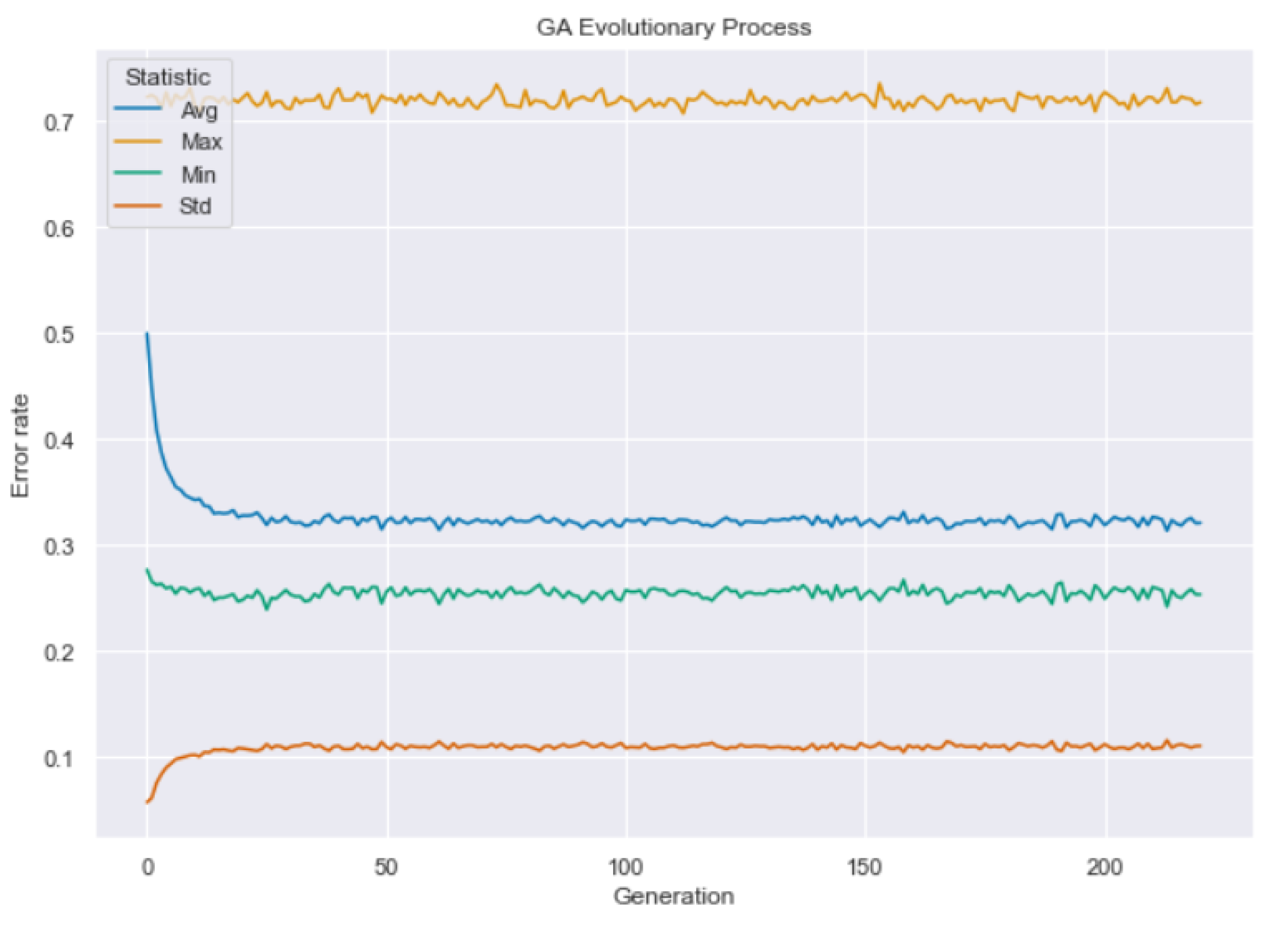
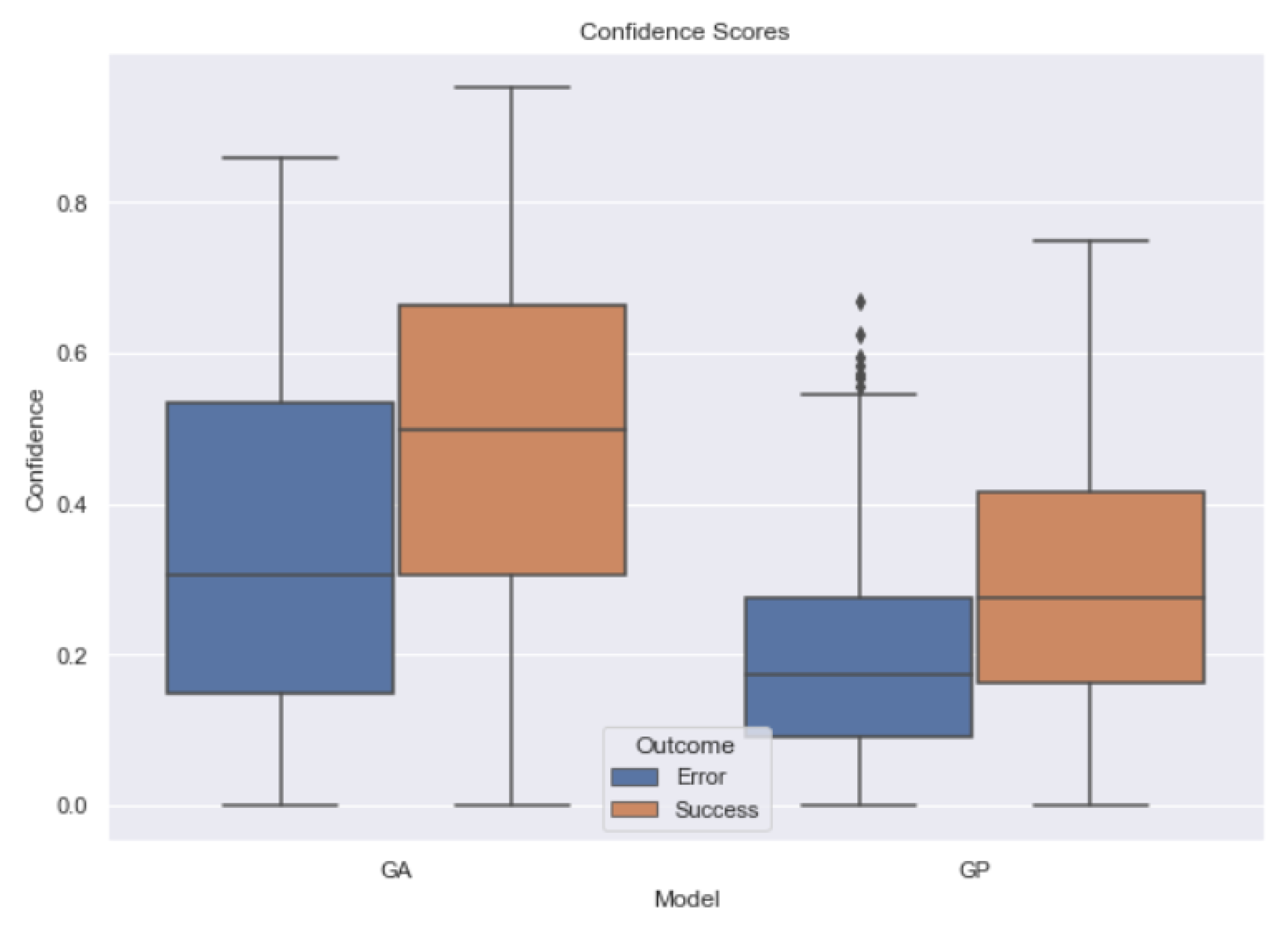
Table 1.
Features that characterize each user profile on Twitter according to our classification models.
Table 1.
Features that characterize each user profile on Twitter according to our classification models.
| ID | Feature Name |
|---|---|
| reputation | |
| listed growth rate | |
| favorites growth rate | |
| friends growth rate | |
| followers growth rate | |
| statuses growth rate | |
| screen name length | |
| frequency of words | |
| frequency of hashtags | |
| frequency of mentioned users | |
| frequency of retweets | |
| frequency of URLs | |
| words raw counts standard dev. | |
| hashtags raw counts standard dev. | |
| mentioned users raw counts standard dev. | |
| tweets similarities mean | |
| tweets lengths standard dev. |
Table 2.
Table that describes the absolute values of the weights learned using GA for each feature. In particular, the weights associated with the human category have a positive sign, while the weights associated with the bot category have a negative sign. We highlight in bold the weights associated with the most important features, while we highlight in gray the weights associated with the least meaningful features.
| ID | Name | Learned Weight | Favored Category |
|---|---|---|---|
| reputation | 1.65 | Human | |
| listed growth rate | 1.50 | Human | |
| favorites growth rate | 0.13 | Human | |
| friends growth rate | 0.54 | Bot | |
| followers growth rate | 1.67 | Human | |
| statuses growth rate | 1.32 | Bot | |
| screen name length | 0.03 | Human | |
| frequency of words | 0.37 | Bot | |
| frequency of hashtags | 0.71 | Bot | |
| frequency of mentioned users | 0.61 | Bot | |
| frequency of retweets | 0.93 | Bot | |
| frequency of URLs | 1.74 | Bot | |
| words raw counts standard dev. | 1.66 | Bot | |
| hashtags raw counts standard dev. | 0.13 | Bot | |
| mentioned users raw counts standard dev. | 0.68 | Human | |
| tweets similarities mean | 0.40 | Bot | |
| tweets lengths standard dev. | 0.77 | Human |
Table 3.
The table shows the components of the formula learned using GP.
| Component ID | Component Formula | Favored Category |
|---|---|---|
| Human | ||
| Human | ||
| Human | ||
| Bot | ||
| Bot | ||
| Bot |
Table 4.
The table describes the components of the formula learned using GP.
| Component ID | Component Description |
|---|---|
| Combination of listed growth rate and reputation | |
| Weighted followers growth rate | |
| Weighted mentioned users raw counts standard deviation | |
| Weighted frequency of hashtags | |
| Mean between frequency of retweets and frequency of URLs | |
| Words raw counts standard deviation weighted by screen name length |
Table 5.
Performance of the baseline methods on TwiBot-20 test set with respect to the accuracy, F1 score, and MCC, together with qualitative performance of the GA model and the GP model. Each of these models has been trained using the training set, validated using the validation set, and tested for a final assessment using the test set. The results related to the baseline methods are based on the results presented in [6]. For each chosen evaluation metric, we highlight in bold the highest value.
| GA | GP | Yang et al. [36] | Kudugunta et al. [44] | Wei et al. [45] | Cresci et al. [19] | Botometer [38] | Alhosseini et al. [43] | Miller et al. [23] | Lee at al. [37] | |
|---|---|---|---|---|---|---|---|---|---|---|
| Accuracy | 0.76 | 0.76 | 0.82 | 0.82 | 0.71 | 0.48 | 0.56 | 0.68 | 0.48 | 0.75 |
| F1 score | 0.78 | 0.78 | 0.85 | 0.75 | 0.75 | 0.11 | 0.49 | 0.73 | 0.63 | 0.78 |
| MCC | 0.51 | 0.52 | 0.66 | 0.67 | 0.42 | 0.08 | 0.16 | 0.35 | −0.14 | 0.49 |
Table 6.
Description of the types of information that the described models leverage to perform their predictions.
Table 6.
Description of the types of information that the described models leverage to perform their predictions.
| GA | GP | Yang et al. [36] | Kudugunta et al. [44] | Wei et al. [45] | Cresci et al. [19] | Botometer [38] | Alhosseini et al. [43] | Miller et al. [23] | Lee at al. [37] | |
|---|---|---|---|---|---|---|---|---|---|---|
| Meta-data | ✓ | ✓ | ✓ | ✓ | ✓ | ✓ | ✓ | ✓ | ||
| Tweets | ✓ | ✓ | ✓ | ✓ | ✓ | ✓ | ✓ | ✓ | ||
| Neighbors | ✓ | ✓ |
Table 7.
Mean and standard deviation of multiple executions of the training procedures based on GA and GP.
Table 7.
Mean and standard deviation of multiple executions of the training procedures based on GA and GP.
| GA | GP | ||
|---|---|---|---|
| Accuracy | Mean | 0.7511 | 0.7660 |
| Std dev. | 0.0045 | 0.0070 | |
| F1 score | Mean | 0.7789 | 0.7884 |
| Std dev. | 0.0032 | 0.0067 | |
| MCC | Mean | 0.4974 | 0.5278 |
| Std dev. | 0.0092 | 0.0140 | |
Table 8.
Set of possible Pareto frontiers generated by executing different evolutionary processes with different weights for the fitness function. The final models were evaluated using the TwiBot-20 test set.
Table 8.
Set of possible Pareto frontiers generated by executing different evolutionary processes with different weights for the fitness function. The final models were evaluated using the TwiBot-20 test set.
| Seed | Max Depth | MSE Weight | Size Weight | Size | Accuracy | F1 | MCC |
|---|---|---|---|---|---|---|---|
| 1 | 16 | 0.95 | 0.05 | 97 | 0.7796 | 0.7945 | 0.5409 |
| 2 | 14 | 0.90 | 0.10 | 116 | 0.7701 | 0.7943 | 0.5357 |
| 3 | 12 | 0.85 | 0.15 | 54 | 0.7667 | 0.7896 | 0.5289 |
| 4 | 11 | 0.80 | 0.20 | 70 | 0.7650 | 0.7891 | 0.5254 |
| 5 | 10 | 0.75 | 0.25 | 64 | 0.7642 | 0.7859 | 0.5240 |
| 6 | 9 | 0.70 | 0.30 | 65 | 0.7796 | 0.7920 | 0.5414 |
| 7 | 8 | 0.65 | 0.25 | 65 | 0.7701 | 0.7930 | 0.5357 |
| 8 | 7 | 0.60 | 0.40 | 44 | 0.7557 | 0.7758 | 0.5075 |
| 9 | 6 | 0.50 | 0.50 | 26 | 0.7616 | 0.7797 | 0.5200 |
| 10 | 5 | 0.40 | 0.60 | 27 | 0.7608 | 0.7874 | 0.5168 |
| 11 | 4 | 0.30 | 0.70 | 16 | 0.7430 | 0.7686 | 0.4809 |
| 12 | 4 | 0.20 | 0.80 | 14 | 0.7557 | 0.7772 | 0.5071 |
Publisher’s Note: MDPI stays neutral with regard to jurisdictional claims in published maps and institutional affiliations. |
© 2022 by the authors. Licensee MDPI, Basel, Switzerland. This article is an open access article distributed under the terms and conditions of the Creative Commons Attribution (CC BY) license (https://creativecommons.org/licenses/by/4.0/).
Share and Cite
MDPI and ACS Style
Rovito, L.; Bonin, L.; Manzoni, L.; De Lorenzo, A. An Evolutionary Computation Approach for Twitter Bot Detection. Appl. Sci. 2022, 12, 5915. https://doi.org/10.3390/app12125915
AMA Style
Rovito L, Bonin L, Manzoni L, De Lorenzo A. An Evolutionary Computation Approach for Twitter Bot Detection. Applied Sciences. 2022; 12(12):5915. https://doi.org/10.3390/app12125915
Chicago/Turabian StyleRovito, Luigi, Lorenzo Bonin, Luca Manzoni, and Andrea De Lorenzo. 2022. "An Evolutionary Computation Approach for Twitter Bot Detection" Applied Sciences 12, no. 12: 5915. https://doi.org/10.3390/app12125915
Note that from the first issue of 2016, this journal uses article numbers instead of page numbers. See further details here.