
Enhanced Intrusion Detection with Data Stream Classification and Concept Drift Guided by the Incremental Learning Genetic Programming Combiner
 , , , , and
Abstract
:1. Introduction
- To the best of our knowledge, this paper provides the first data stream-based classification framework that addresses CD variants.
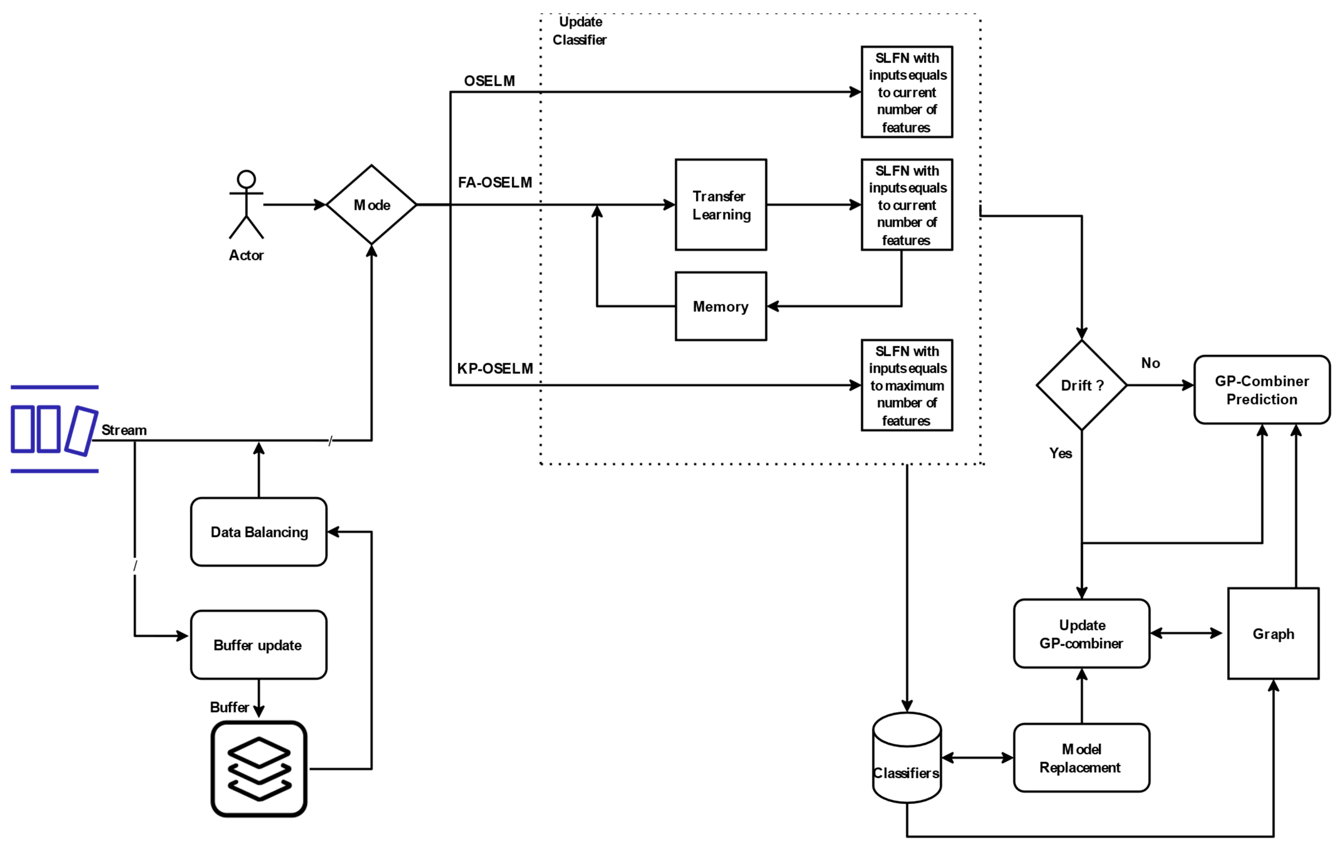
- It provides various novel strategies for handling CD, such as using an ensemble learning-based GPC, incremental learning using online sequential extreme learning machine (OSELM), and transfer learning (TL).
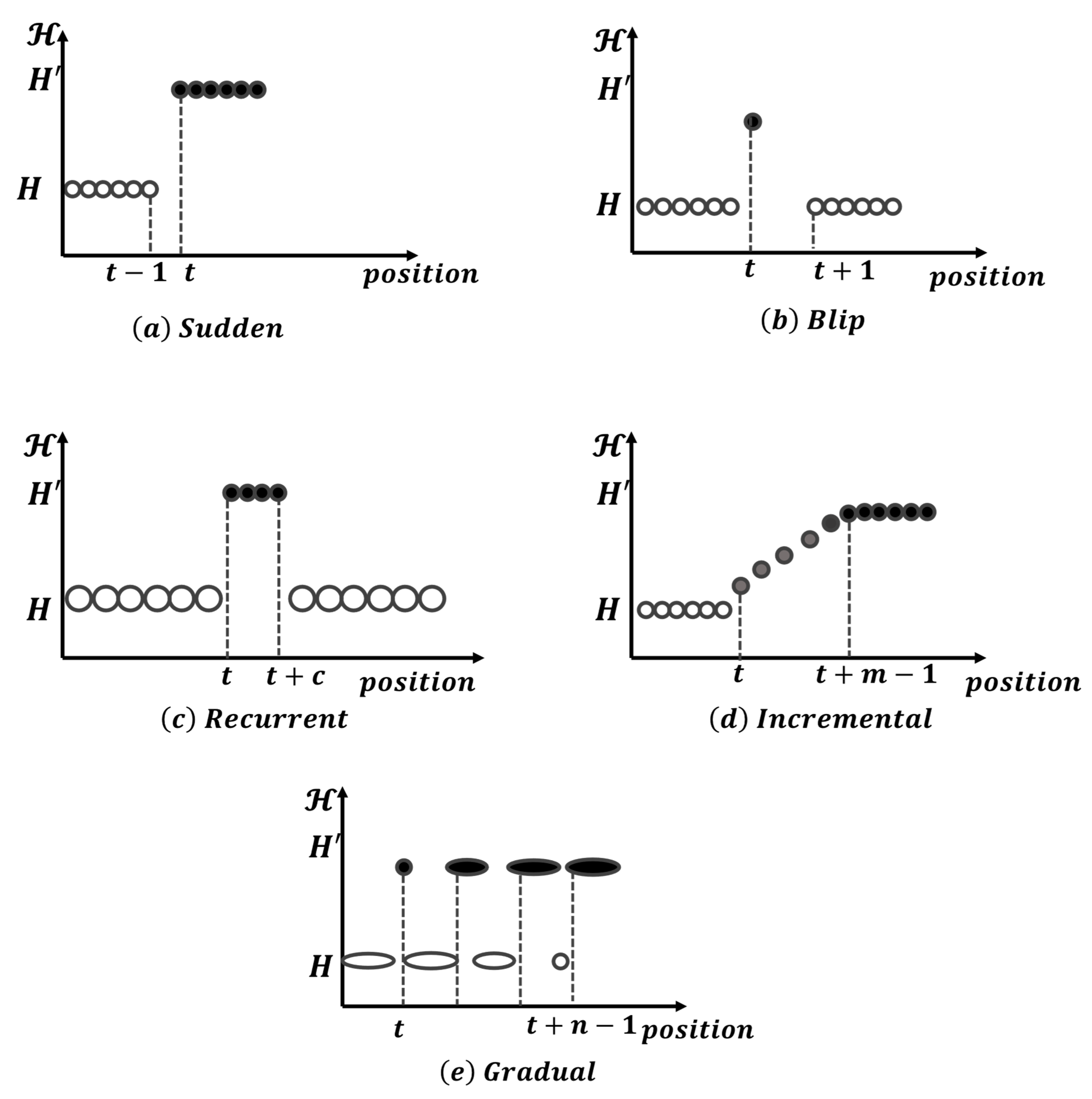
- It proposes the usage of knowledge preservation OSELM (KP-OSELM) to contend with certain variants of drift that require restoring previous memory, such as sudden, recurrent, and gradual.
- Two novel components are added to the GPC: data balancing and classifiers update. Additionally, a specific coordination between the various sub-models in an incremental GPC is proposed.
- It provides an evaluation of two types of data: synthetic data and real-world data. The real-world data belong to more than one field, with a focus on network IDS. The evaluation includes a comparison against several state-of-the-art methods and the usage of time series classification.
2. Literature Survey
2.1. CD-Aware IDS Methods
2.2. CD-Aware Methods
2.3. Literature Gap
3. Background
3.1. Background of OSELM, FA-OSELM and KP-OSELM
3.1.1. OSELM Review
Where: hi = [g (W1. Xi + b1),…, g (WÑ. Xi + bÑ)]T, i = 1,…,
| Algorithm 1. The pseudocode of the ELM (OS-ELM) algorithm. |
| Input: (1) ℵ = {(Xi, ti)|Xi Rn, ti Rm, i = 1,... , Ñ} Output: trained SLFN Start Algorithm 1: Boosting Phase: 2: Assign arbitrary input weight and bias or center and impact width . 3: Calculate the initial hidden layer output matrix in Equation (1) 4: Estimate the initial output weight (0) = M0T0, Where M0 = (H0)−1 and T0 = [t1,...,tÑ]T. 5: Set . 6: Sequential Learning Phase: 7: For each further coming observation (Xi, ti), where, Xi Rn, ti ; Rm and i = Ñ + 1, Ñ + 2, Ñ + 3,…, do 8: Calculate the hidden layer output vector in Equation (2) 9: Calculate latest output weight (k+1) based on RLS Equation (3) 10: Set . 11: end 12: End Algorithm |
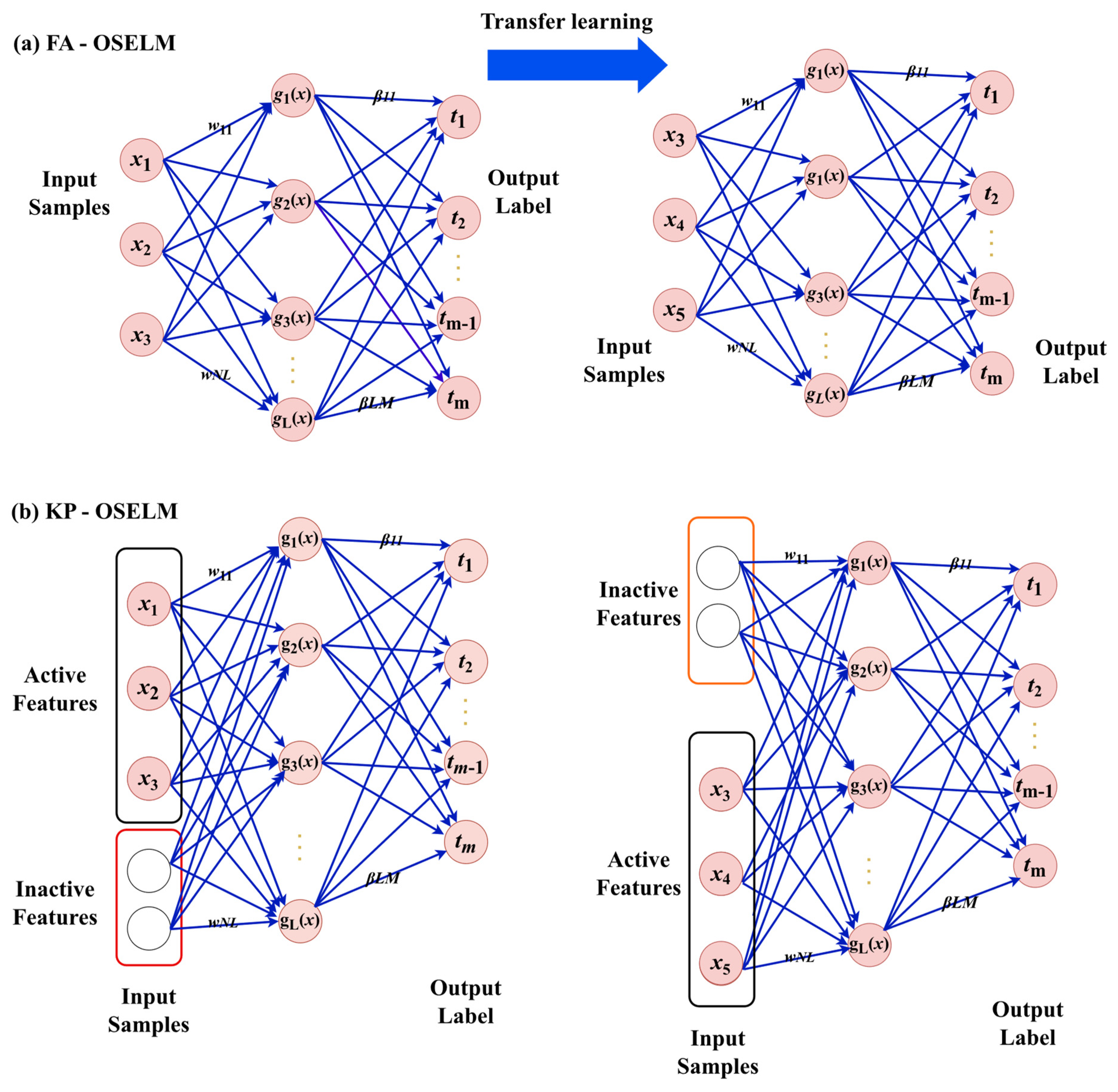
3.1.2. FA-OSELM Review
- For every line, there is a single ‘1’; the rest of the values are all ‘0’.
- Every column has no more than a single ‘1’; the rest of the values are all ‘0’.
- signifies that following a change in the feature dimension, the dimension of the original feature vector will become the dimension of the new feature vector.
- When the feature dimension increases, will function as the supplement. It also adds the corresponding input weight for the newly added attributes. Furthermore, the rules below apply to .
- Lower feature dimensions indicate that can be termed as an all-zero vector. Hence, no additional corresponding input weight is required by the newly added features.
- In cases where the feature dimension increases, if the new feature is embodied by the item of , a random generation of the item of should be carried out based on the distribution of .
3.1.3. KP-OSELM Review
| Algorithm 2. The pseudocode for training and prediction using KP-OSELM. |
| Input: (1) (2) Output: (1) ACC Start: 1.: x0 = Encode (D0) 2.: SLFN1 = OSELMTrain (SLFN0, x0, y0) 3: for k = 1 unit N 4: 5: 6: 7: 8: end 9: End Algorithm |
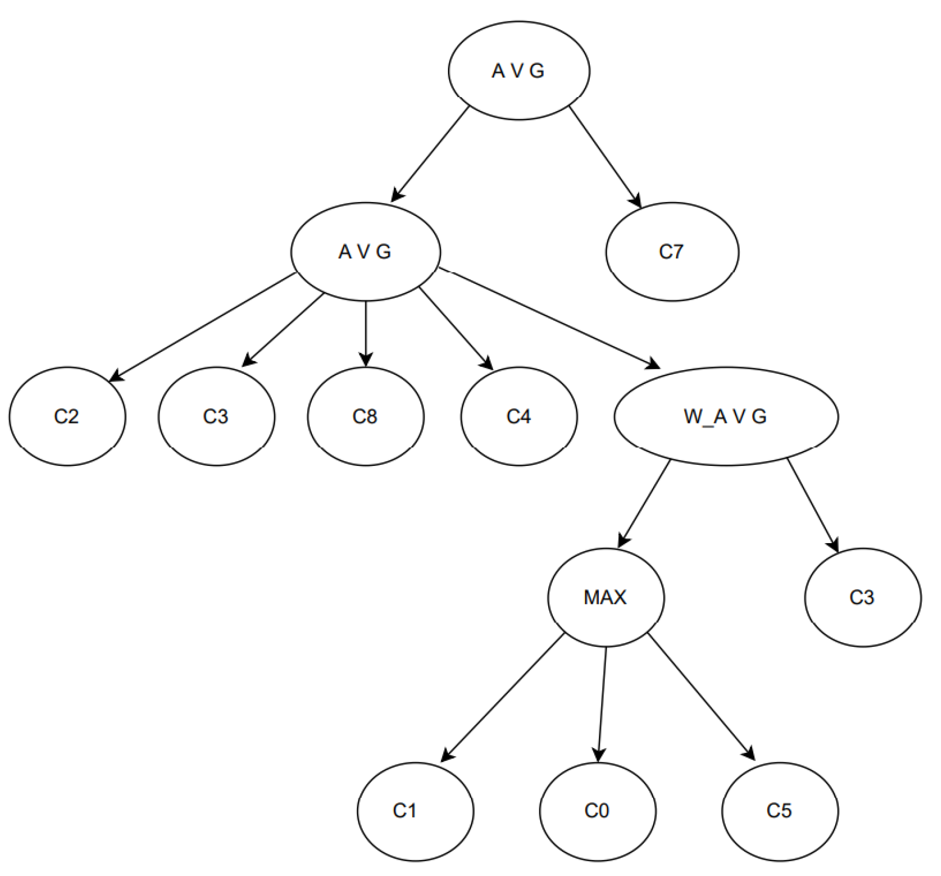
3.2. GPC
| Algorithm 3. Pseudocode of GPC. |
| Input: (1) x: an instance from the data stream (2) y: the corresponding label of x (3) buffer: a list of instances (4) ensemble: an ensemble data structure (5) DDO: a drift detection object (6) maxC: the maximum number of classifiers in the ensemble (7) n: the number of instances in the buffer to apply model induction after exceeding it (8) drift: a Boolean variable indicating a drift occurrence (9) NumHiddenNeurons, (10) ActivationFunc Output: (1) ensemble: the updated ensemble (2) buffer: the updated buffer (3) drift: the updated drift flag Start Algorithm 1: If (ensemble==Null) 2: classifiers = initialisation(NumHiddenNeurons,ActivationFunc); // Algorithm 4 3: ensemble = createEnsemble(classifiers); 4: End 5: ypred = globalSupportDegree(ensemble, x) // Algorithm 5 6: if y! = None then 7: buffer.append((x, y)) 8: drift = DDO.detect(x, y! = ypred 9: if len(buffer) >= n then 10: if drift: 11: drift = False 12: buffer = addExamplesFromAnotherClass(buffer) 13: = trainTestSplit(buffer) 14: newClassifiers = modelInduction(, generateClassifiers()) 15: ensemble.baseClassifiers = ensemble.baseClassifiers = baseClassifierUpdate(ensemble.baseClassifiers, newClassifiers, X_1, X_2, L = maxC, Key = ‘validScore’) // Algorithm 6 16: if len(ensemble.baseClassifiers) > maxC then 17: ensemble.baseClassifiers = modelReplacement(ensemble.baseClassifiers, method = ‘best’) //Algorithm 7 18: ensemble.program = geneticProgramming(ensemble.baseClassifiers, ) ensemble.baseClassifiers = modelReplacement(ensemble.baseClassifiers, method = ‘best’) //Algorithm 7 19: End 20: Else 21: buffer.clear() 22: return ensemble, buffer, drift 23: End 24: end 25: End Algorithm |
4. Methodology
4.1. Problem Formulation
4.2. Incremental Learning GPC
4.3. Initialisation
| Algorithm 4. Pseudocode of initialisation of the incremental GPC with classifier. |
| Input: (1) NumHiddenNeurons: number of hidden neurons to be used in the classifier (2) ActivationFunc: activation function to be used in the classifier Output: (1) classifiers: list of machine learning models to be used in ensemble 1: Start Algorithm 2: classifiers = list() 3: for index = 1 until NumHiddenNeurons 4: classifiers.Append(OSELM(NumHiddenNeurons(index), ActivationFunc(index))) 5: end 6: Return classifiers 7: End Algorithm |
4.4. Prediction Using Global Support Degree
| Algorithm 5. Pseudocode of global support degree for the incremental GPC. |
| Input: (1) baseClassifiers: custom data structure to store classifiers (2) sample: new instance from the data Output: (1) decisionProfile: support degree, 2D array contains prediction probability of each classifier (2) ypred 1: Start Algorithm 2: decisionProfile = [] // Initialize decision profile list 3: for each clf in baseClassifiers do // Iterate over each classifier in the base classifiers 4: decisionProfile.add(clf.predictProbability(sample)) 5: end for 6: decisionProfile = array(decisionProfile, shape = (numOfClassifier, numOfClasses)) 7: decisionProfile = argmax(decisionProfile.sum(axis = 0)/decisionProfile.shape [0]) 8: ypred = class of max decisionProfile 9: End Algorithm |
4.5. BaseClassifier Update
| Algorithm 6. Pseudocode of classifier update for the incremental GPC. |
| Input: (1) baseClassifiers: list of existing classifiers (2) newClassifiers: list of new classifiers to be added (3) Xtrain: training data (4) XValid: validation data (5) L: maximum number of classifiers to be kept (6) Key: sorting key for the classifiers (7) LabeledSamples: labeled samples for incremental learning Output: (1) baseClassifiers: updated list of classifiers 1: Start Algorithm 2: for each clf in newClassifiers do 3: use LabeledSamples to update classifier incrementally for OSELM and with TL for FA-OSELM and KP-OSELM 4: clf.trainScore = accuracy(clf.predict(Xtrain), ytrain) 5: clf.validScore = accuracy(clf.predict(XValid), yvalid) 6: clf.insertionTime = time.currTime() 7: end 8: newClassifiers = sort(newClassifiers, key) 9: newClassifiers = newClassifiers[:L] 10: for each clf in newClassifiers do 11 baseClassifiers.insert(clf) 12: end 13: End Algorithm |
4.6. Model Replacement
| Algorithm 7. Pseudocode of model replacement for the incremental GPC. |
| Input: (1) baseClassifiers: list of existing classifiers (2) method: string that determines the replacement method to be used Output: (1) baseClassifiers: updated list of classifiers after replacement 1: Start Algorithm 2: strategy = {‘best’: ‘validScore’, ‘random’: ‘insertionTime’, ‘wheel’: ‘validScore’} 3: key = strategy[method] 4: baseClassifiers = sort(baseClassifiers, key = key) 5: length = len(baseClassifiers) 6: threshold = length/3 7: baseClassifiers = baseClassifiers [0:threshold] 8: End Algorithm |
4.7. Evaluation Metrics
4.7.1. Accuracy
4.7.2. F-Score
4.7.3. AUC
4.8. Datasets
4.8.1. Synthetic Datasets
4.8.2. Real-World Datasets
- KDD Cup ‘99: Frequently used to test threat detection models based on ML and contains 42 features for evaluating anomaly detection methods [45].
- CICIDS-2017: Covers benign and up-to-date frequent attacks and contains 80 features [46].
- CSE-CIC-IDS-2018: Contains 80 features and was employed in 2018, with a data collection period of ten days [46].
- ISCX2012: Comprises 19 features and is well recognised for its use of ML-based network IDS modelling for evaluating the performance of the models [47].
5. Experimental Works and Results
5.1. Synthetic Datasets
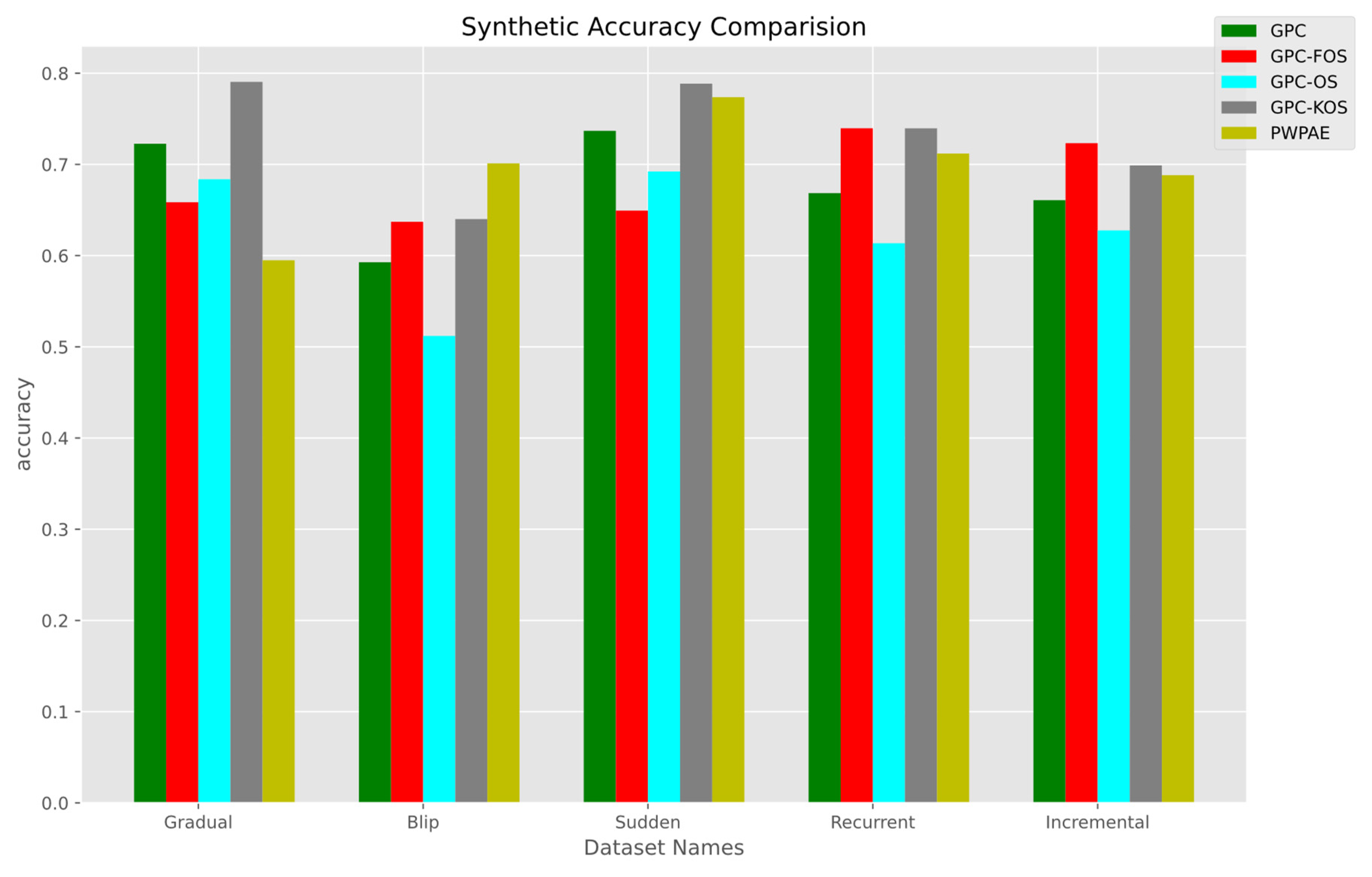
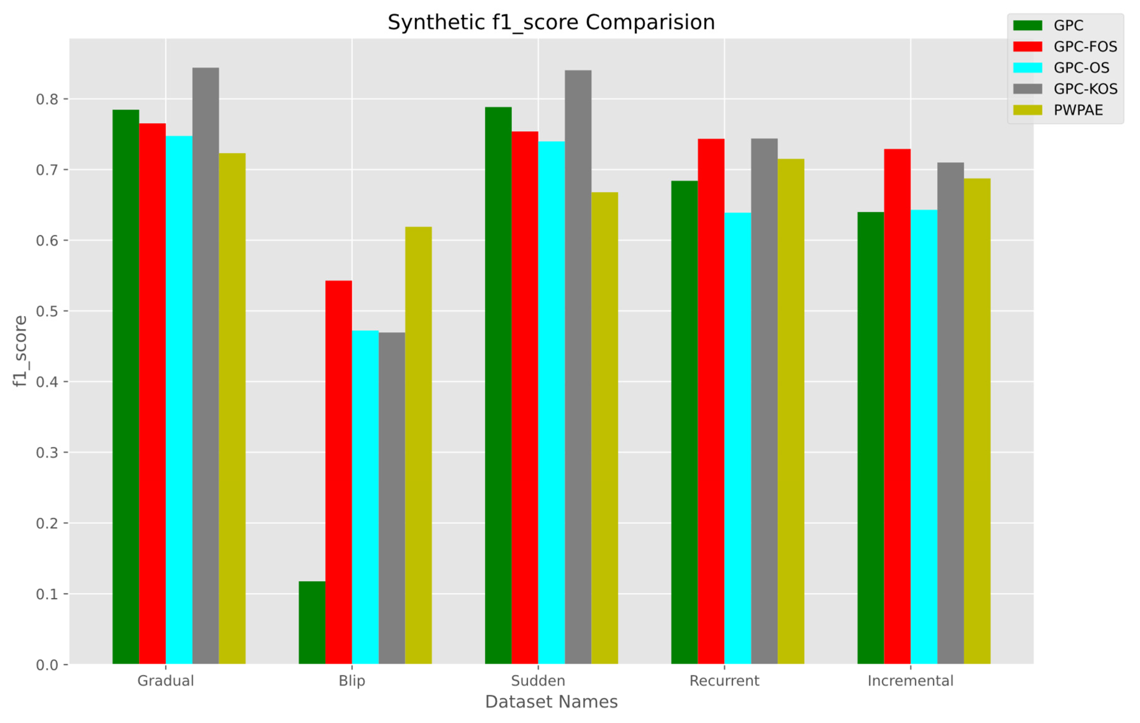
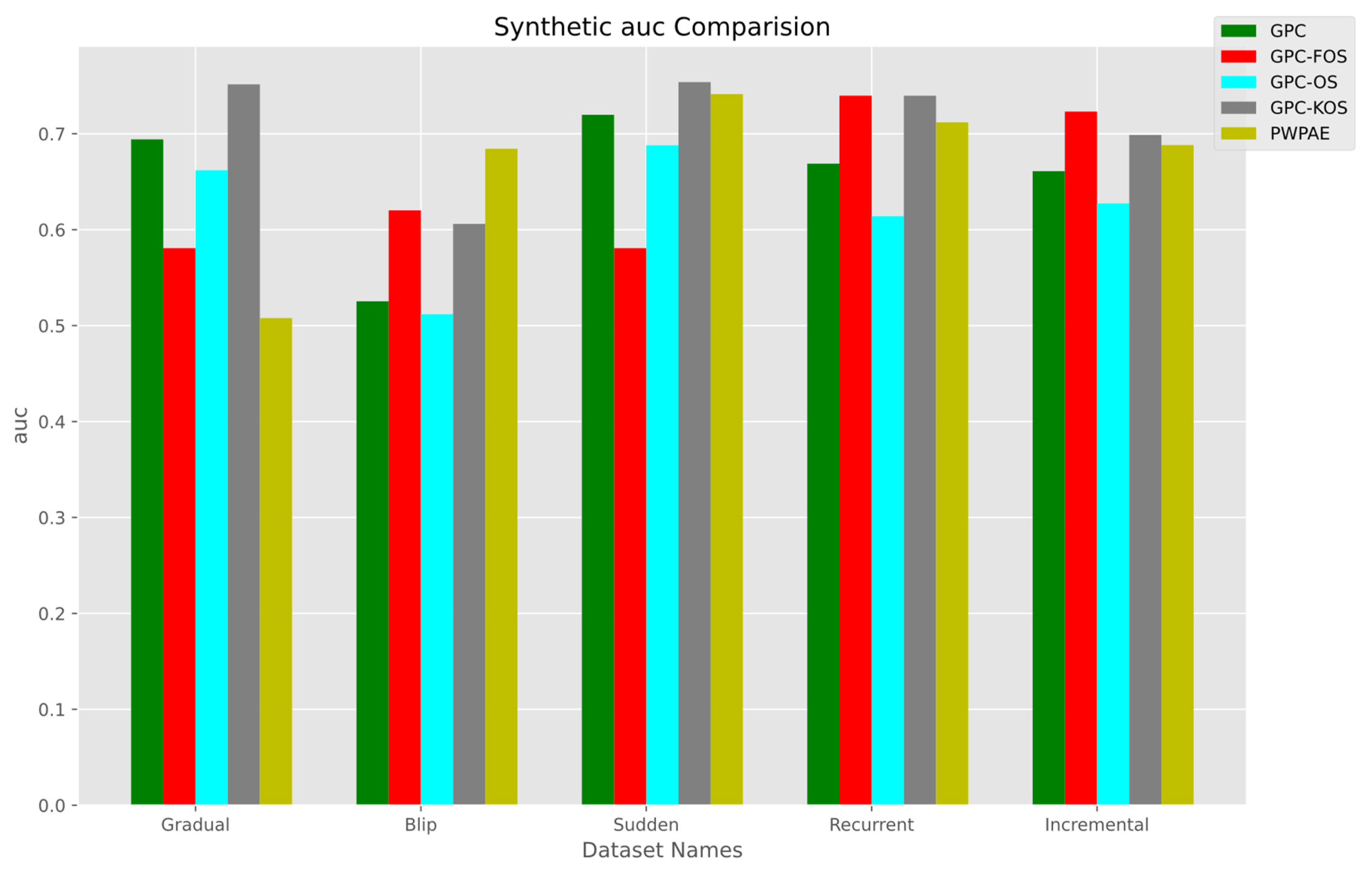
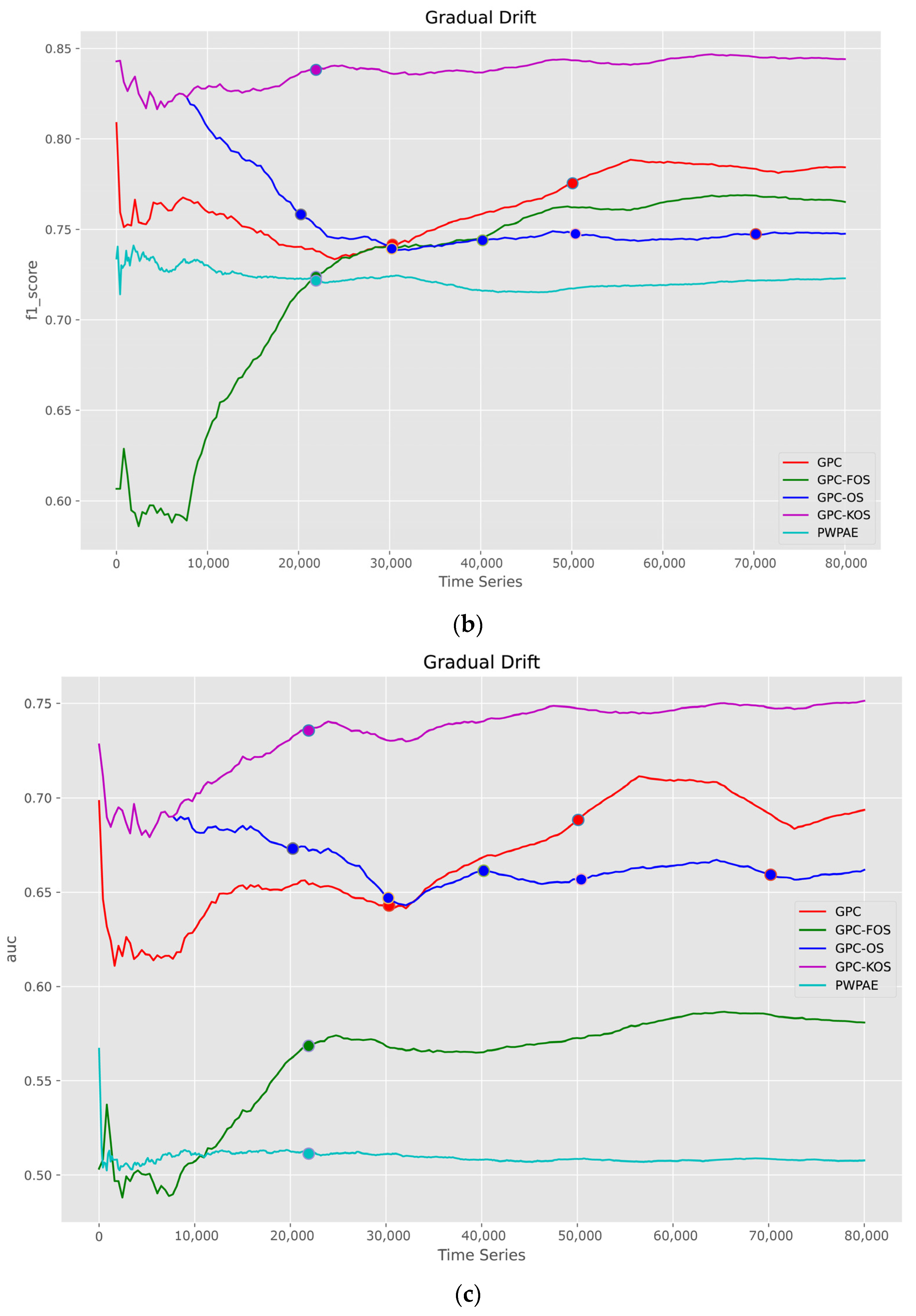
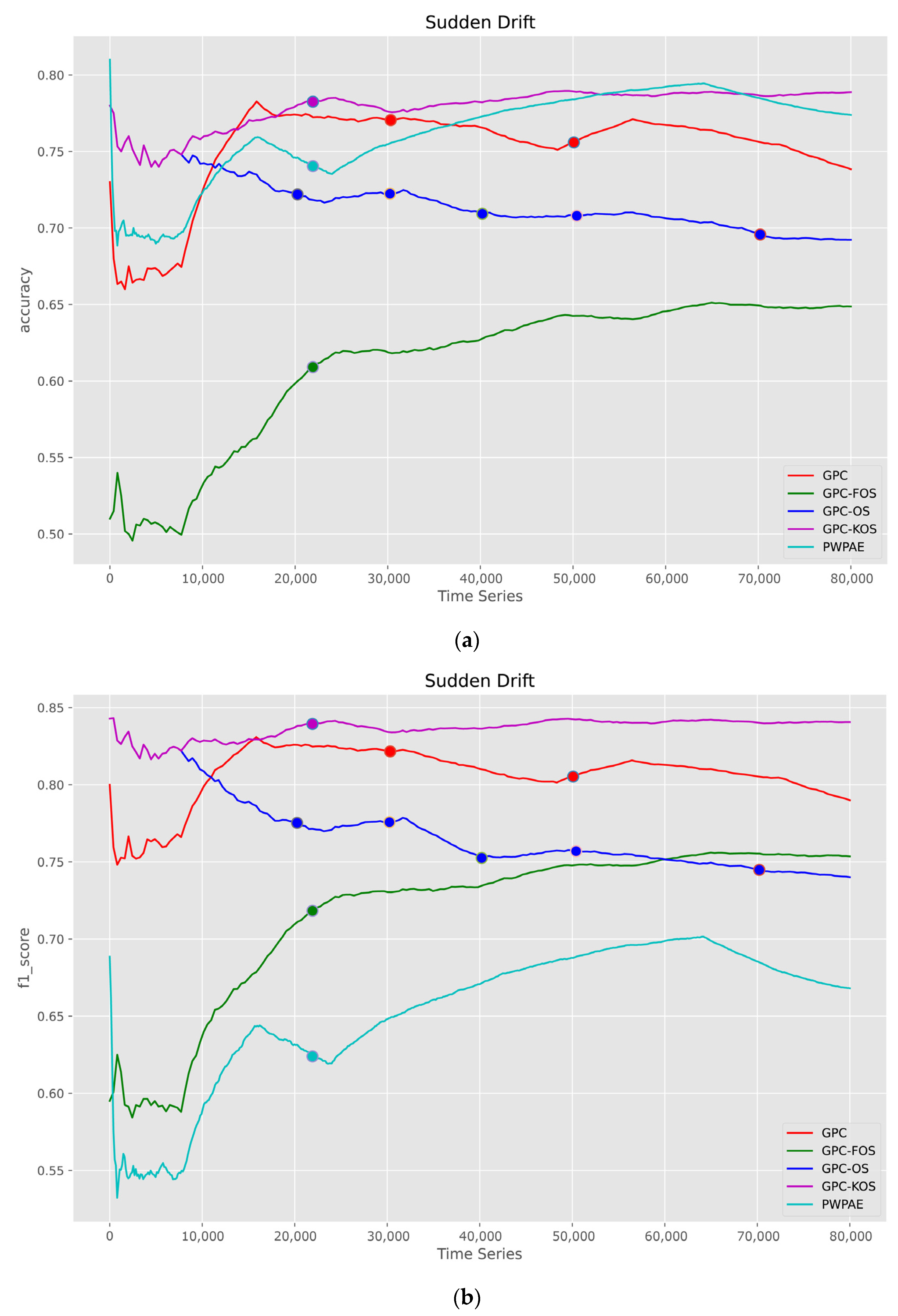
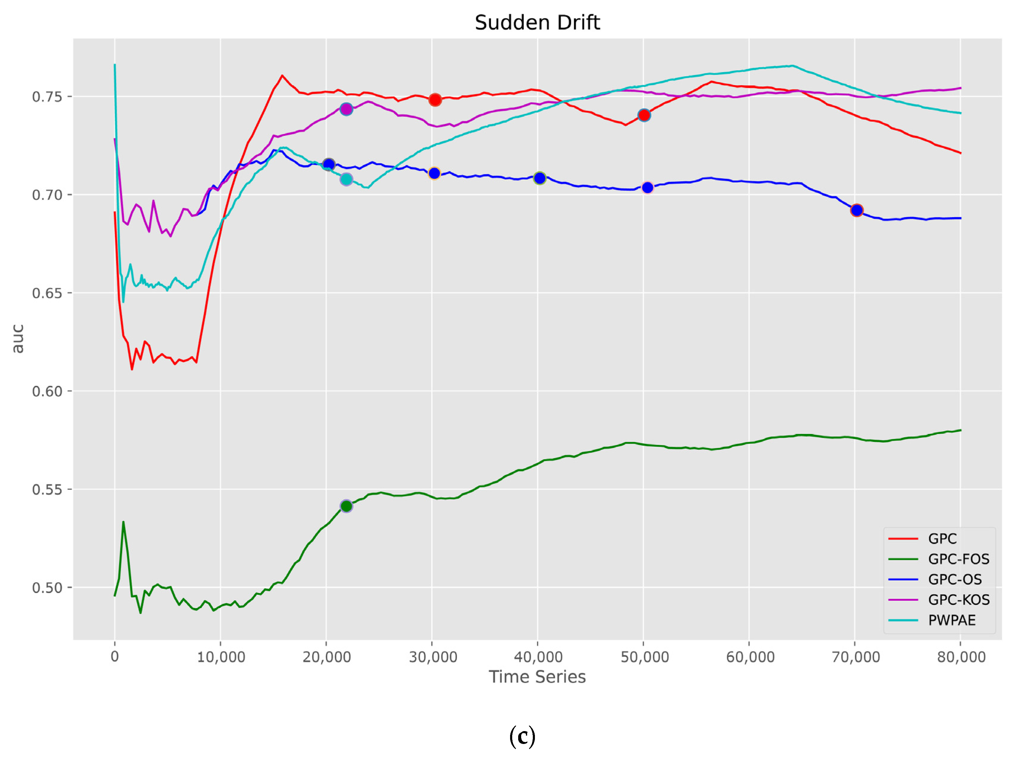
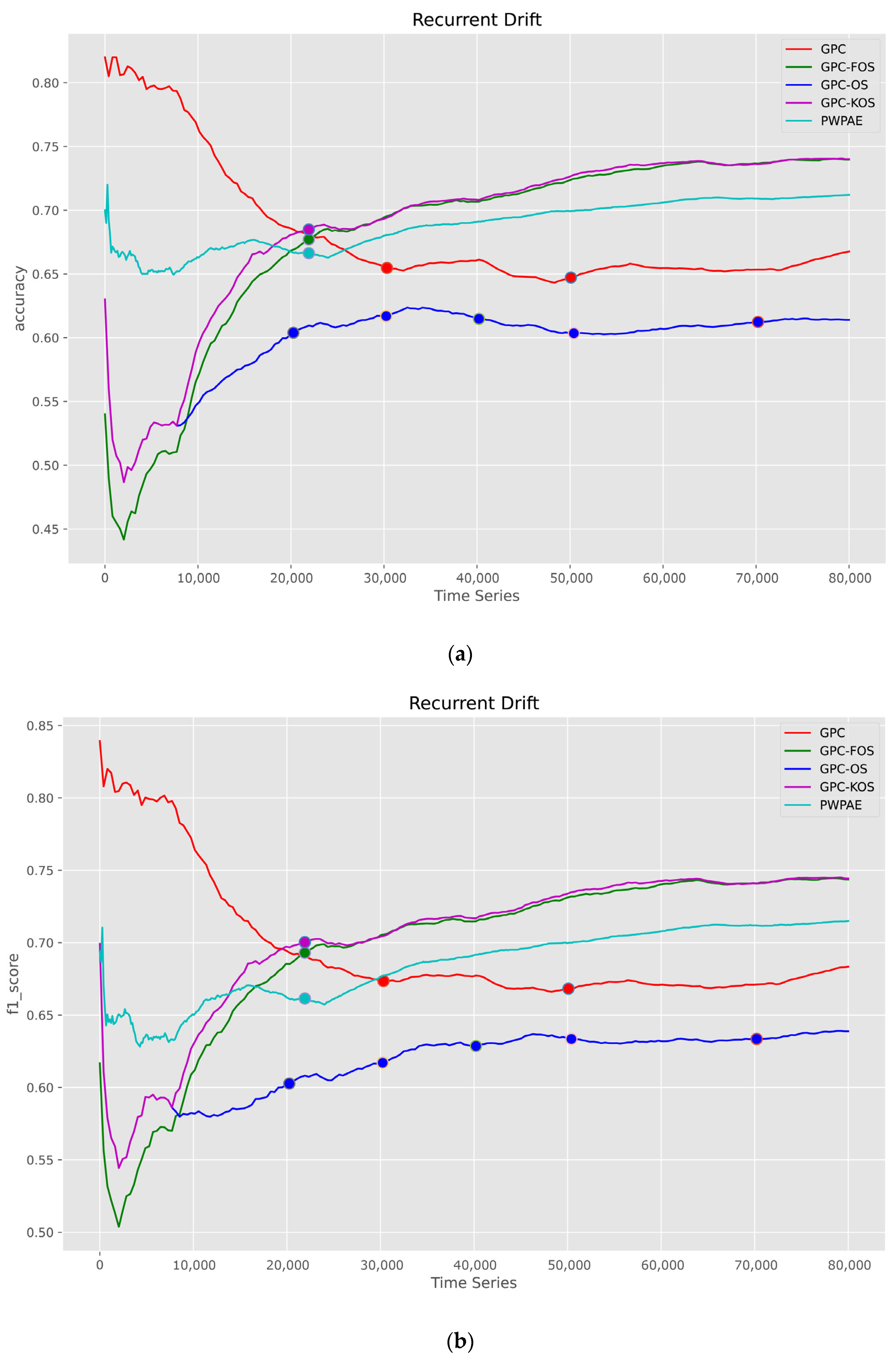
5.1.1. Overall Performance
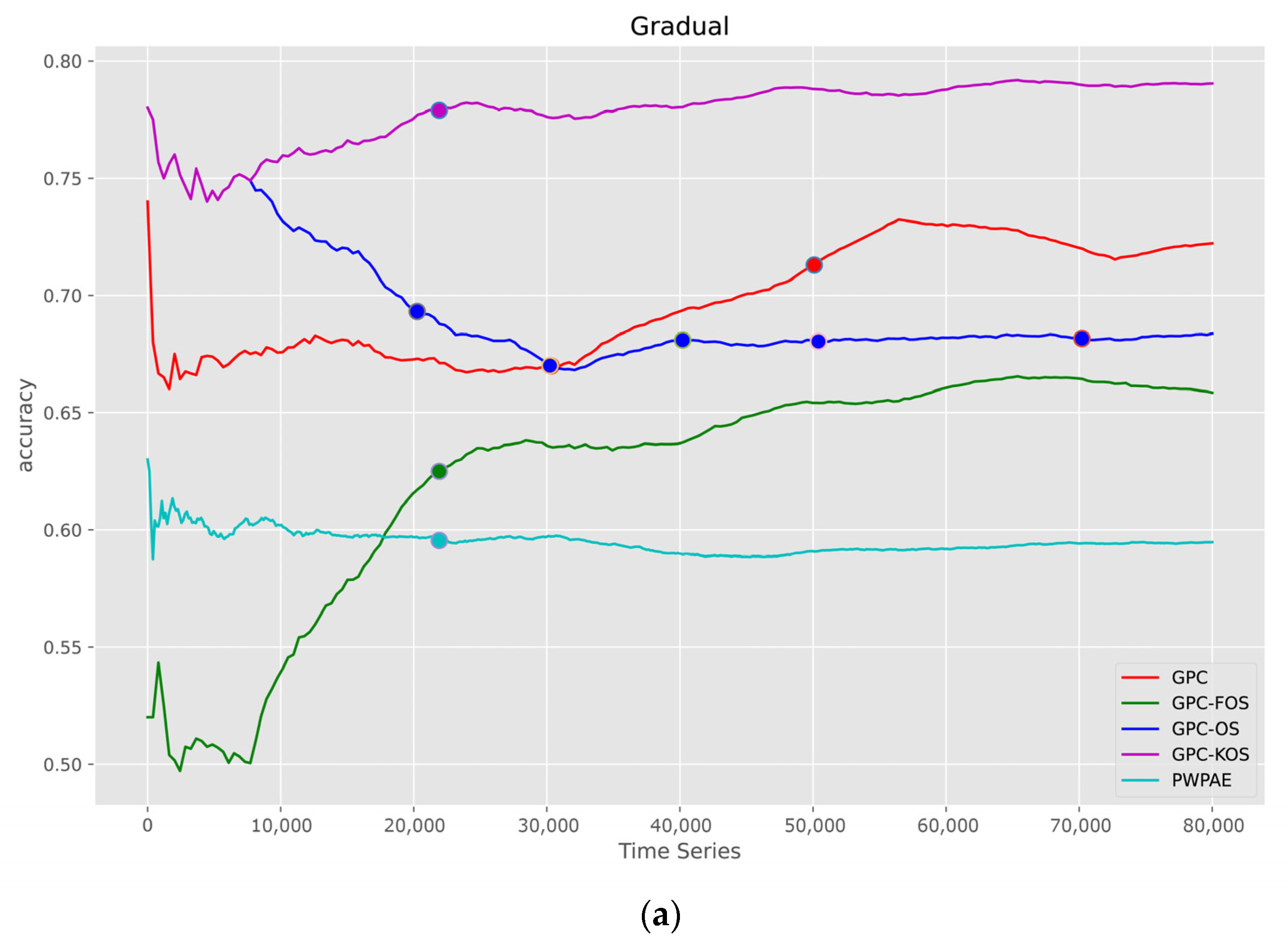
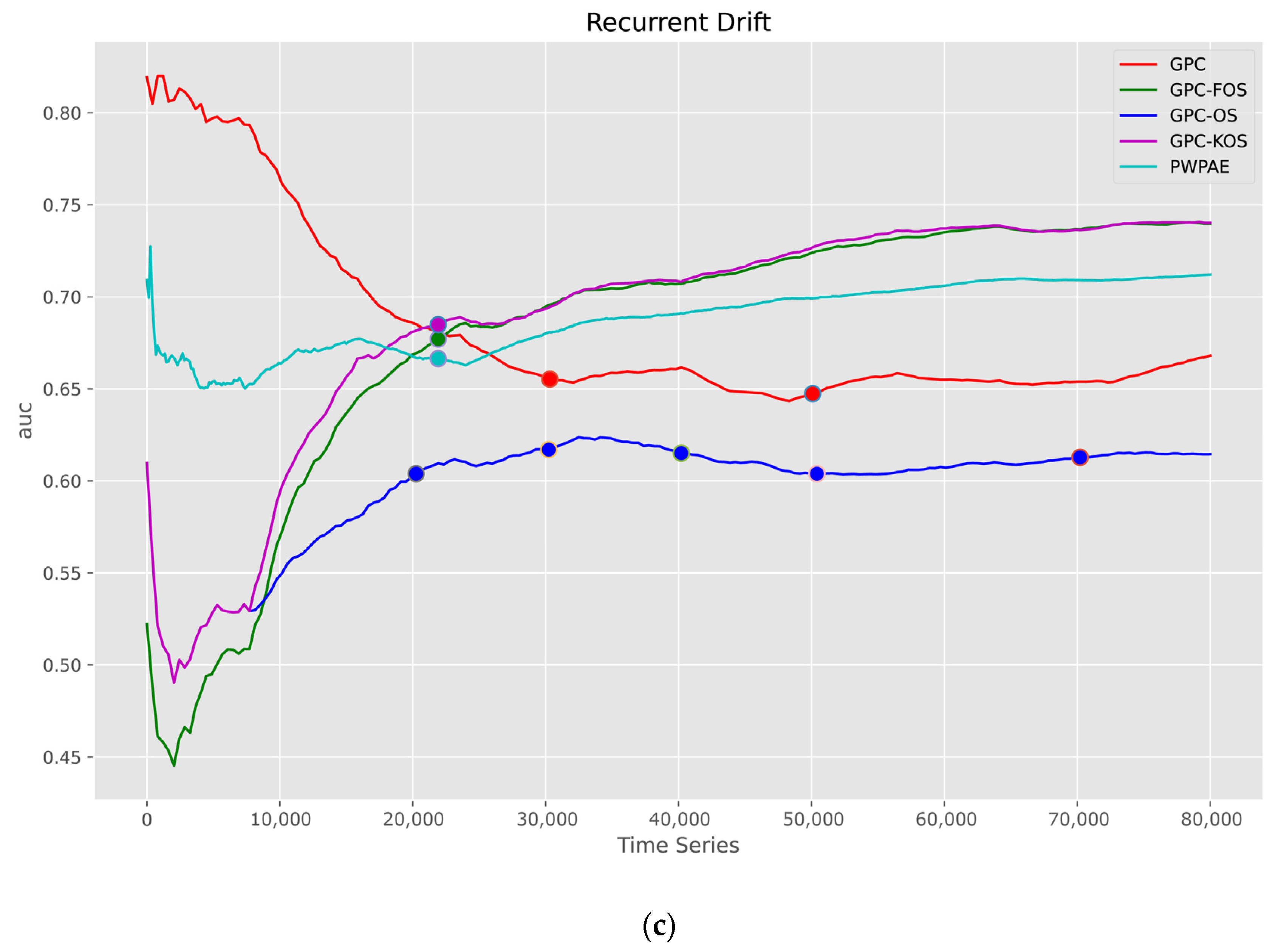
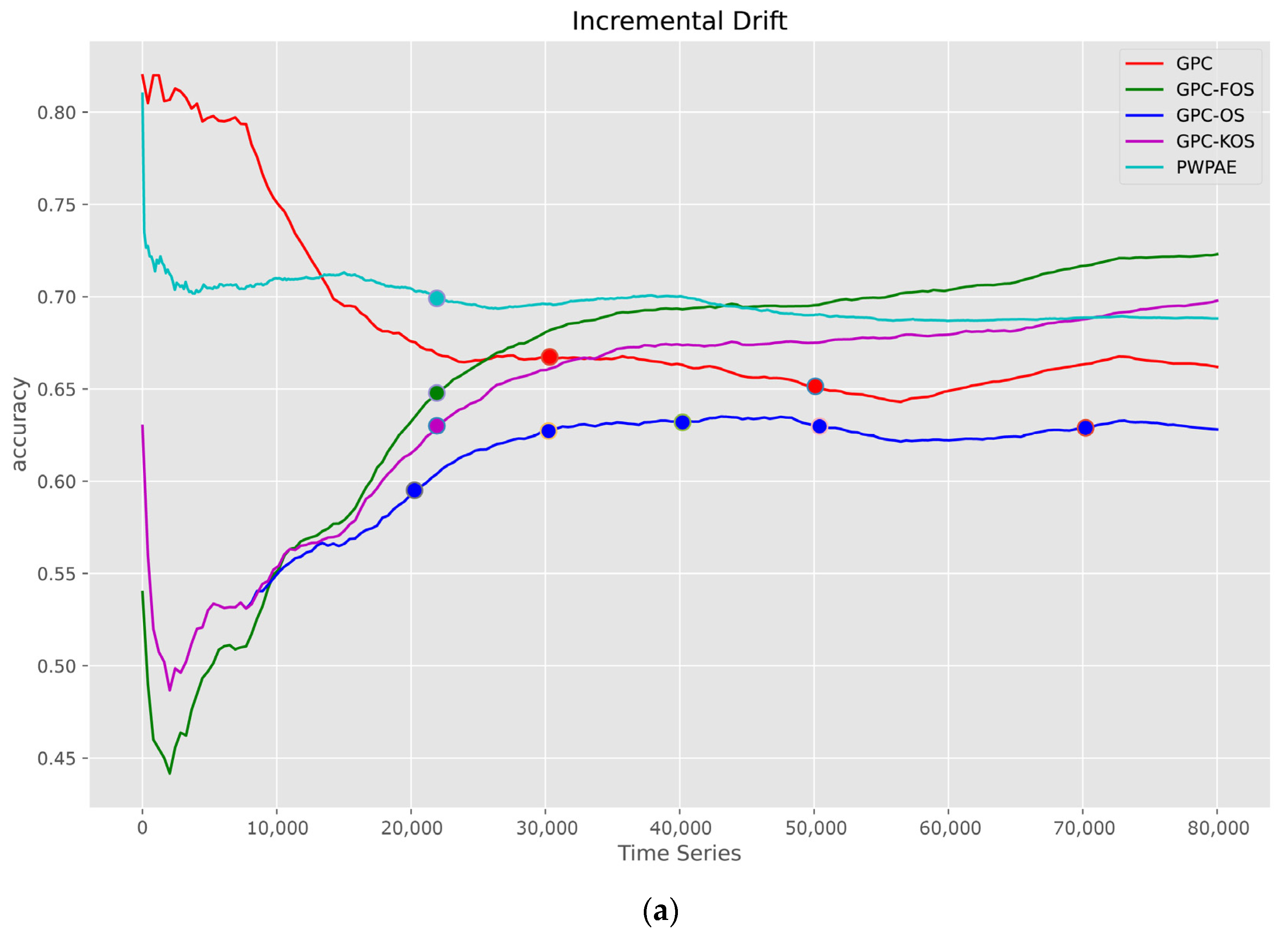
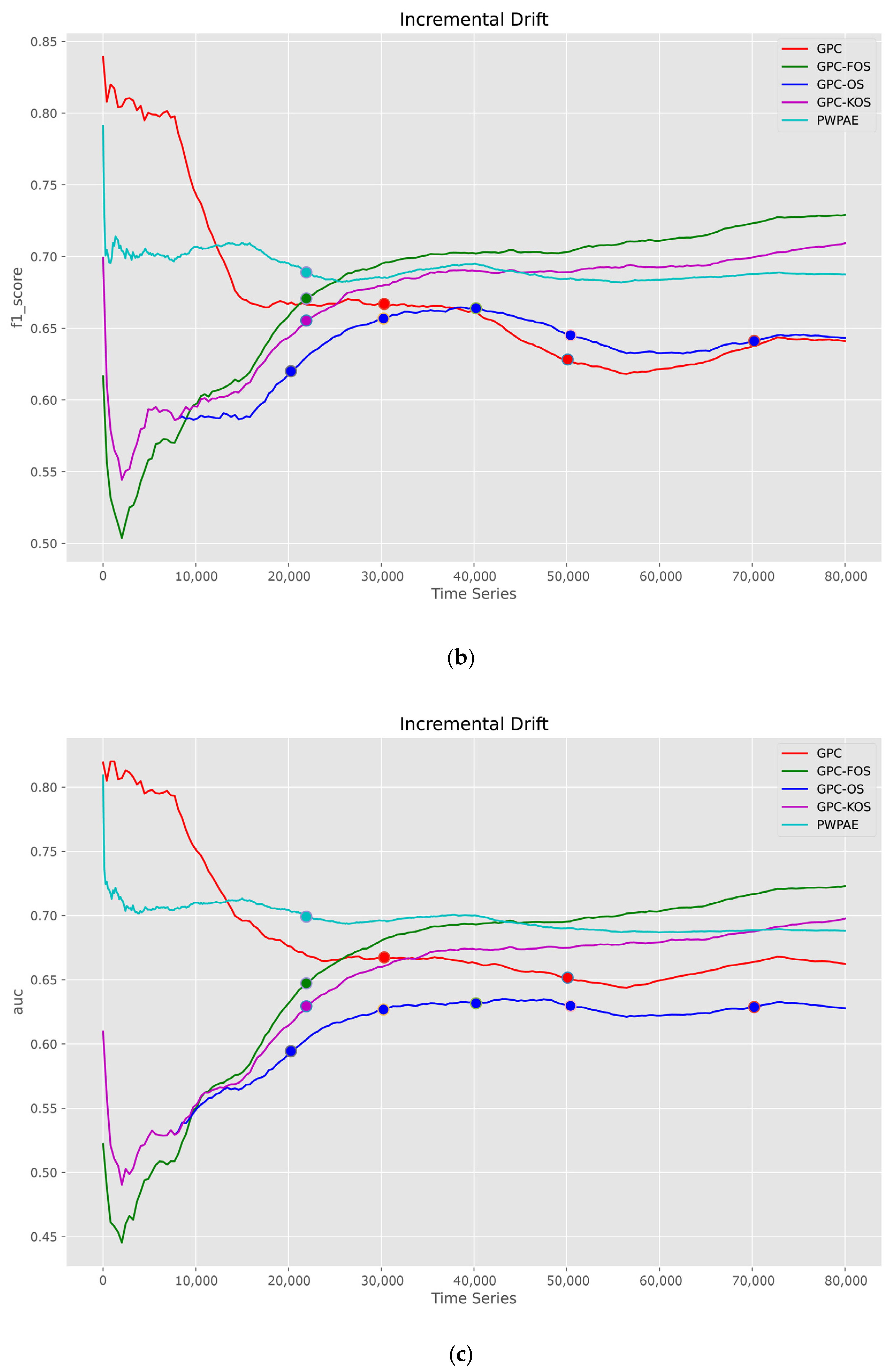
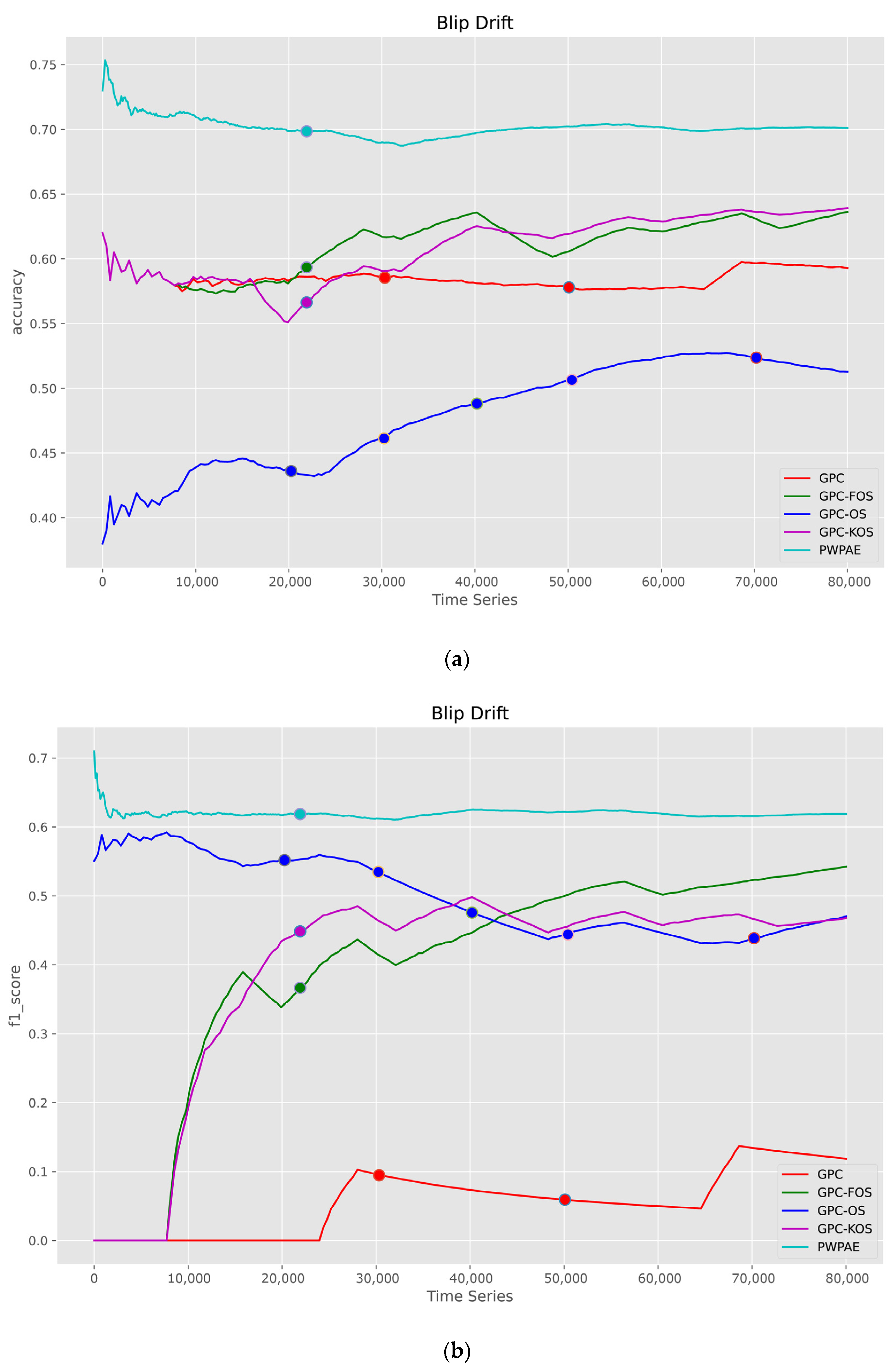
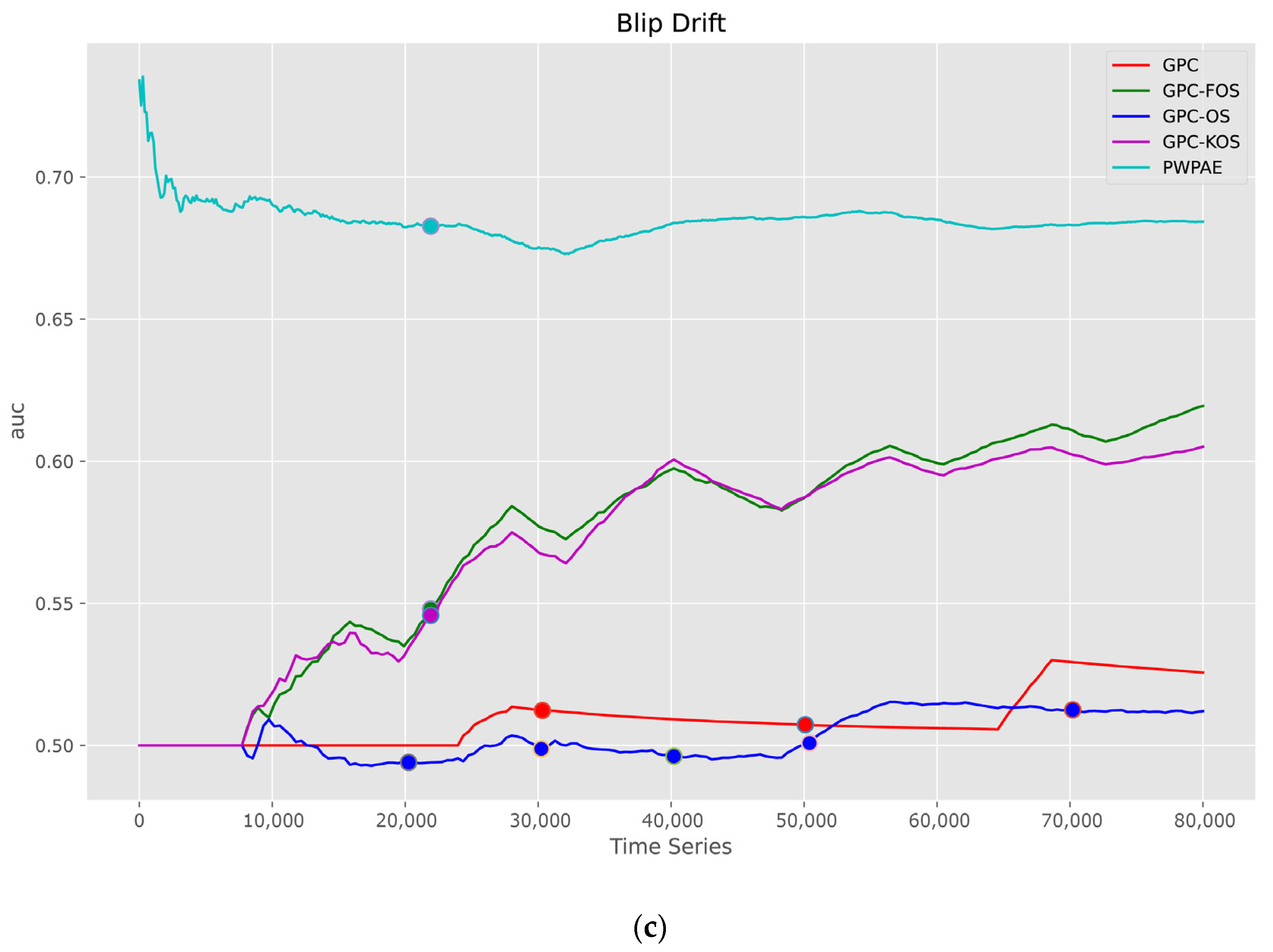
5.1.2. Time Series
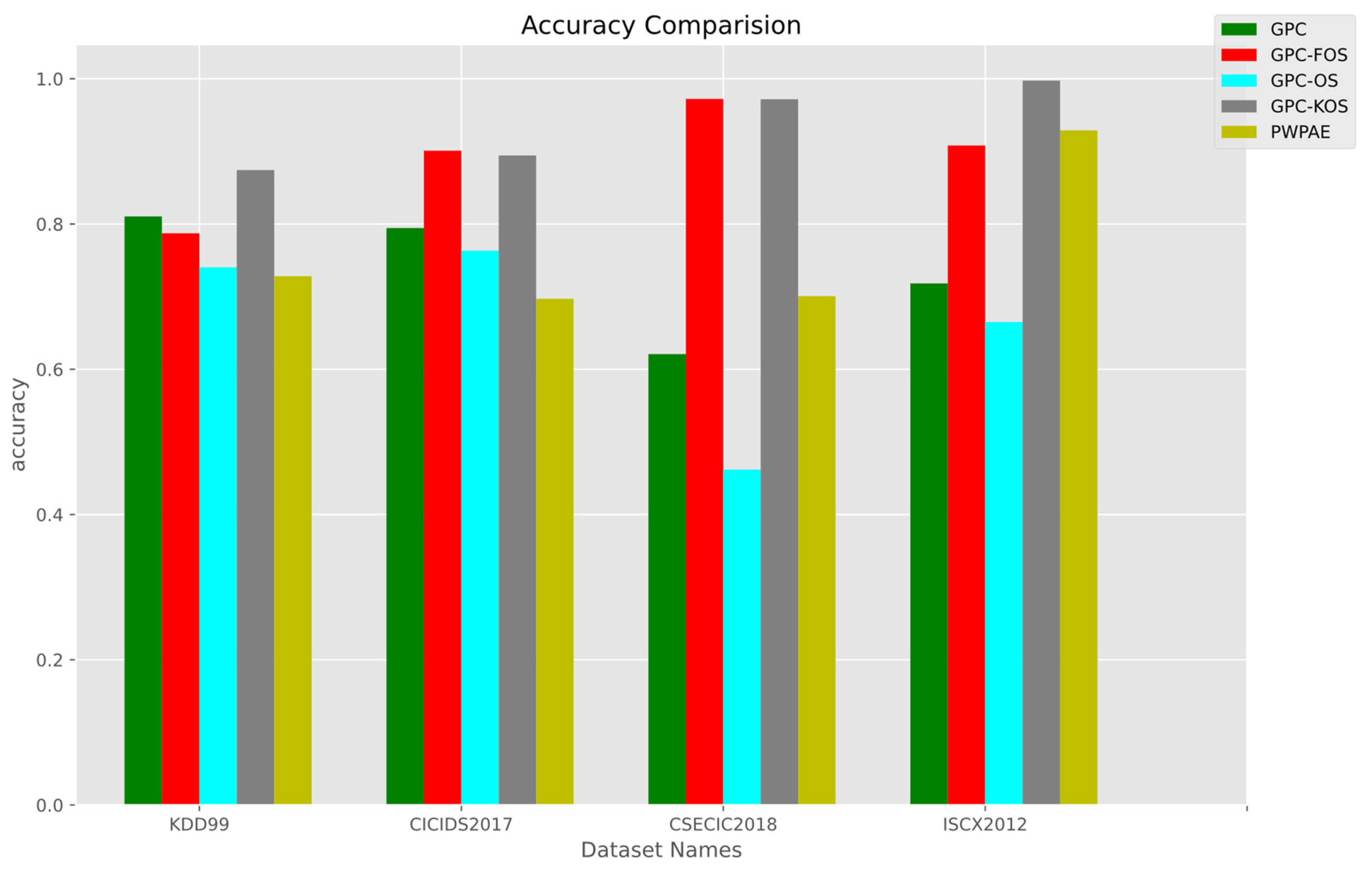
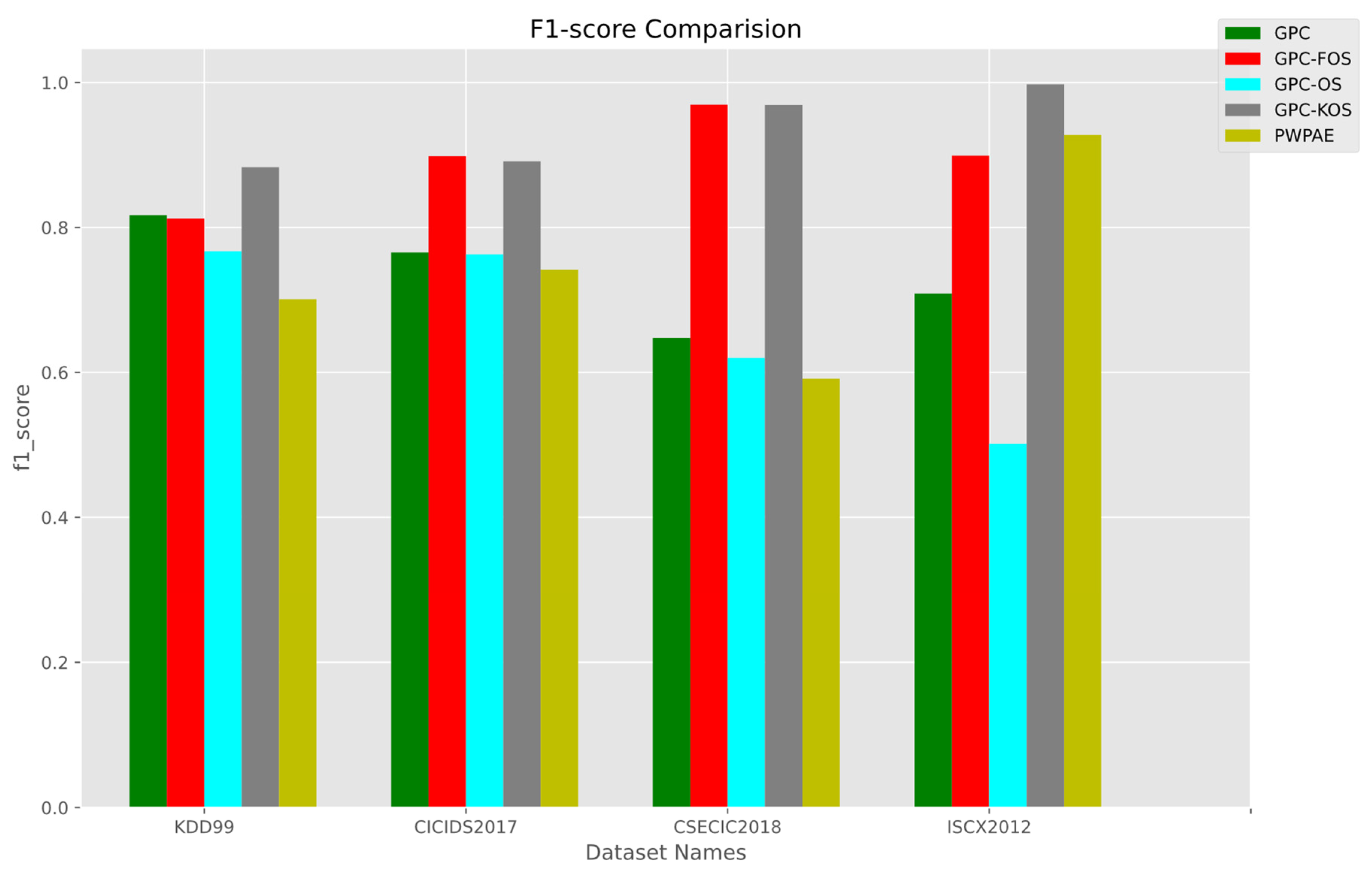
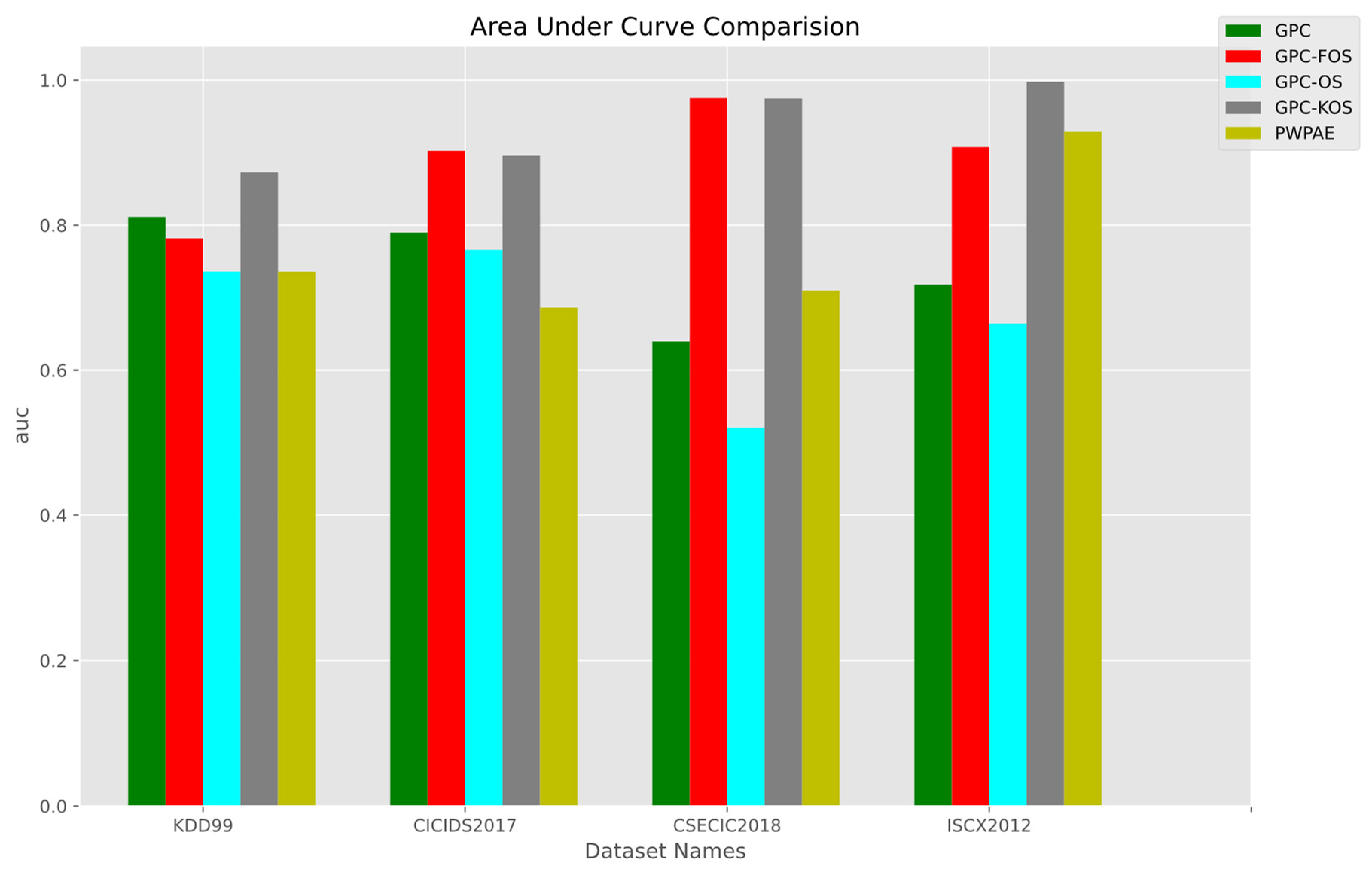
5.2. Real-World Datasets IDS
Overall Results
6. Advantages of the Incremental GPC
- Improved performance in handling different CD variants: Our proposed framework provides novel strategies for handling different types of CD, such as incremental, sudden, recurrent, gradual, and blip. This results in improved classification performance compared to the traditional GPC and other state-of-the-art methods.
- Memory features and TL: The proposed framework utilises TL and memory features, which allow the model to retain previous knowledge and adapt to incoming data. This results in improved performance in handling CD and reduces the need for retraining the model from scratch.
- Enhanced data balancing and classifier update: The addition of data balancing and classifier update components to the GPC model further improves the accuracy of classification.
- Real-world applicability: The proposed framework has been tested on real-world datasets, specifically in the context of a network IDS, which is a critical application in cybersecurity. This highlights the practical applicability of the proposed framework in real-world scenarios.
- Comprehensive evaluation: Our work provides a comprehensive evaluation of the proposed framework on both synthetic and real-world datasets using standard classification metrics as time series, which allows for a fair and objective comparison against other state-of-the-art methods.
7. Conclusions and Future Works
Author Contributions
Funding
Institutional Review Board Statement
Informed Consent Statement
Data Availability Statement
Conflicts of Interest
References
- Yazdi, H.S.; Bafghi, A.G. A drift aware adaptive method based on minimum uncertainty for anomaly detection in social networking. Expert Syst. Appl. 2020, 162, 113881. [Google Scholar]
- Jain, M.; Kaur, G. Distributed anomaly detection using concept drift detection based hybrid ensemble techniques in streamed network data. Clust. Comput. 2021, 24, 2099–2114. [Google Scholar] [CrossRef]
- Zhang, Z.; Chen, L.; Liu, Q.; Wang, P. A fraud detection method for low-frequency transaction. IEEE Access 2020, 8, 25210–25220. [Google Scholar] [CrossRef]
- Mansour, R.F.; Al-Otaibi, S.; Al-Rasheed, A.; Aljuaid, H.; Pustokhina, I.; Pustokhin, D.A. An optimal big data analytics with concept drift detection on high-dimensional streaming data. CMC Comput. Mater. Contin. 2021, 68, 2843–2858. [Google Scholar] [CrossRef]
- Neto, A.F.; Canuto, A.M. EOCD: An ensemble optimization approach for concept drift applications. Inf. Sci. 2021, 561, 81–100. [Google Scholar] [CrossRef]
- Wang, S.; Minku, L.L.; Yao, X. A systematic study of online class imbalance learning with concept drift. IEEE Trans. Neural Netw. Learn. Syst. 2018, 29, 4802–4821. [Google Scholar] [CrossRef]
- Kalid, S.N.; Ng, K.-H.; Tong, G.-K.; Khor, K.-C. A multiple classifiers system for anomaly detection in credit card data with unbalanced and overlapped classes. IEEE Access 2020, 8, 28210–28221. [Google Scholar] [CrossRef]
- Sarnovsky, M.; Kolarik, M. Classification of the drifting data streams using heterogeneous diversified dynamic class-weighted ensemble. Peer J. Comput. Sci. 2021, 7, e459. [Google Scholar] [CrossRef]
- Chi, H.R.; Wu, C.K.; Huang, N.-F.; Tsang, K.F.; Radwan, A. A Survey of Network Automation for Industrial Internet-of-Things Towards Industry 5.0. IEEE Trans. Ind. Inform. 2022, 19, 2065–2077. [Google Scholar] [CrossRef]
- Leng, J.; Sha, W.; Wang, B.; Zheng, P.; Zhuang, C.; Liu, Q.; Wuest, T.; Mourtzis, D.; Wang, L. Industry 5.0: Prospect and retrospect. J. Manuf. Syst. 2022, 65, 279–295. [Google Scholar] [CrossRef]
- Demir, K.A.; Döven, G.; Sezen, B. Industry 5.0 and human-robot co-working. Procedia Comput. Sci. 2019, 158, 688–695. [Google Scholar] [CrossRef]
- Angelopoulos, A.; Michailidis, E.T.; Nomikos, N.; Trakadas, P.; Hatziefremidis, A.; Voliotis, S.; Zahariadis, T. Tackling faults in the industry 4.0 era—A survey of machine-learning solutions and key aspects. Sensors 2019, 20, 109. [Google Scholar] [CrossRef] [Green Version]
- Martindale, N.; Ismail, M.; Talbert, D.A. Ensemble-based online machine learning algorithms for network intrusion detection systems using streaming data. Information 2020, 11, 315. [Google Scholar] [CrossRef]
- Adnan, A.; Muhammed, A.; Abd Ghani, A.A.; Abdullah, A.; Hakim, F. An intrusion detection system for the internet of things based on machine learning: Review and challenges. Symmetry 2021, 13, 1011. [Google Scholar] [CrossRef]
- Jain, M.; Kaur, G.; Saxena, V. A K-Means clustering and SVM based hybrid concept drift detection technique for network anomaly detection. Expert Syst. Appl. 2022, 193, 116510. [Google Scholar] [CrossRef]
- Folino, F.; Folino, G.; Guarascio, M.; Pisani, F.S.; Pontieri, L. On learning effective ensembles of deep neural networks for intrusion detection. Inf. Fusion 2021, 72, 48–69. [Google Scholar] [CrossRef]
- Andresini, G.; Pendlebury, F.; Pierazzi, F.; Loglisci, C.; Appice, A.; Cavallaro, L. Insomnia: Towards concept-drift robustness in network intrusion detection. In Proceedings of the 14th ACM Workshop on Artificial Intelligence and Security, Virtual, 15 November 2021; pp. 111–122. [Google Scholar]
- Lu, J.; Liu, A.; Dong, F.; Gu, F.; Gama, J.; Zhang, G. Learning under Concept Drift: A Review. IEEE Trans. Knowl. Data Eng. 2019, 31, 2346–2363. [Google Scholar] [CrossRef] [Green Version]
- Guo, H.; Li, H.; Ren, Q.; Wang, W. Concept drift type identification based on multi-sliding windows. Inf. Sci. 2022, 585, 1–23. [Google Scholar] [CrossRef]
- Seth, S.; Singh, G.; Chahal, K. Drift-based approach for evolving data stream classification in Intrusion detection system. In Proceedings of the Workshop on Computer Networks & Communications, Goa, India, 30 April–1 May 2021; pp. 23–30. [Google Scholar]
- Liu, Q.; Wang, D.; Jia, Y.; Luo, S.; Wang, C. A multi-task based deep learning approach for intrusion detection. Knowl.-Based Syst. 2022, 238, 107852. [Google Scholar] [CrossRef]
- Zhou, Y.; Mazzuchi, T.; Sarkani, S. M-AdaBoost-A based ensemble system for network intrusion detection. Expert Syst. Appl. 2020, 162, 113864. [Google Scholar] [CrossRef]
- Han, B.-H.; Li, Y.-M.; Liu, J.; Geng, S.-L.; Li, H.-Y. Elicitation criterions for restricted intersection of two incomplete soft sets. Knowl.-Based Syst. 2014, 59, 121–131. [Google Scholar] [CrossRef]
- Folino, G.; Pisani, F.S.; Pontieri, L. A GP-based ensemble classification framework for time-changing streams of intrusion detection data. Soft Comput. 2020, 24, 17541–17560. [Google Scholar] [CrossRef]
- Kuppa, A.; Le-Khac, N.-A. Learn to adapt: Robust drift detection in security domain. Comput. Electr. Eng. 2022, 102, 108239. [Google Scholar] [CrossRef]
- Adnan, A.; Muhammed, A.; Abd Ghani, A.A.; Abdullah, A.; Hakim, F. Hyper-heuristic framework for sequential semi-supervised classification based on core clustering. Symmetry 2020, 12, 1292. [Google Scholar] [CrossRef]
- dos Santos, R.R.; Viegas, E.K.; Santin, A.O.; Cogo, V.V. Reinforcement learning for intrusion detection: More model longness and fewer updates. IEEE Trans. Netw. Serv. Manag. 2022. [Google Scholar] [CrossRef]
- Qiao, H.; Novikov, B.; Blech, J.O. Concept Drift Analysis by Dynamic Residual Projection for effectively Detecting Botnet Cyber-attacks in IoT scenarios. IEEE Trans. Ind. Inform. 2021, 18, 3692–3701. [Google Scholar] [CrossRef]
- Yang, L.; Shami, A. A Multi-Stage Automated Online Network Data Stream Analytics Framework for IIoT Systems. IEEE Trans. Ind. Inform. 2022, 19, 2107–2116. [Google Scholar] [CrossRef]
- Wahab, O.A. Intrusion detection in the iot under data and concept drifts: Online deep learning approach. IEEE Internet Things J. 2022, 9, 19706–19716. [Google Scholar] [CrossRef]
- Mahdi, O.A.; Pardede, E.; Ali, N. A hybrid block-based ensemble framework for the multi-class problem to react to different types of drifts. Clust. Comput. 2021, 24, 2327–2340. [Google Scholar] [CrossRef]
- Gâlmeanu, H.; Andonie, R. Concept Drift Adaptation with Incremental–Decremental SVM. Appl. Sci. 2021, 11, 9644. [Google Scholar] [CrossRef]
- Museba, T.; Nelwamondo, F.; Ouahada, K.; Akinola, A. Recurrent adaptive classifier ensemble for handling recurring concept drifts. Appl. Comput. Intell. Soft Comput. 2021, 2021, 5533777. [Google Scholar] [CrossRef]
- Wu, O.; Koh, Y.S.; Dobbie, G.; Lacombe, T. Probabilistic exact adaptive random forest for recurrent concepts in data streams. Int. J. Data Sci. Anal. 2022, 13, 17–32. [Google Scholar] [CrossRef]
- Wu, O.; Koh, Y.S.; Dobbie, G.; Lacombe, T. Nacre: Proactive recurrent concept drift detection in data streams. In Proceedings of the 2021 International Joint Conference on Neural Networks (IJCNN), Shenzhen, China, 18–22 July 2021; pp. 1–8. [Google Scholar]
- Chiu, C.W.; Minku, L.L. A diversity framework for dealing with multiple types of concept drift based on clustering in the model space. IEEE Trans. Neural Netw. Learn. Syst. 2020, 33, 1299–1309. [Google Scholar] [CrossRef]
- Cano, A.; Krawczyk, B. Kappa updated ensemble for drifting data stream mining. Mach. Learn. 2020, 109, 175–218. [Google Scholar] [CrossRef]
- Bakhshi, S.; Ghahramanian, P.; Bonab, H.; Can, F. A Broad Ensemble Learning System for Drifting Stream Classification. arXiv 2021, arXiv:2110.03540. [Google Scholar]
- Yang, L.; Manias, D.M.; Shami, A. PWPAE: An Ensemble Framework for Concept Drift Adaptation in IoT Data Streams. In Proceedings of the 2021 IEEE Global Communications Conference (GLOBECOM), Madrid, Spain, 7–11 December 2021; IEEE: New York, NY, USA, 2021; pp. 1–6. [Google Scholar]
- Wang, K.; Lu, J.; Liu, A.; Song, Y.; Xiong, L.; Zhang, G. Elastic gradient boosting decision tree with adaptive iterations for concept drift adaptation. Neurocomputing 2022, 491, 288–304. [Google Scholar] [CrossRef]
- Huang, G.-B.; Liang, N.-Y.; Rong, H.-J.; Saratchandran, P.; Sundararajan, N. On-line sequential extreme learning machine. Comput. Intell. 2005, 2005, 232–237. [Google Scholar]
- Jiang, X.; Liu, J.; Chen, Y.; Liu, D.; Gu, Y.; Chen, Z. Feature adaptive online sequential extreme learning machine for lifelong indoor localization. Neural Comput. Appl. 2016, 27, 215–225. [Google Scholar] [CrossRef]
- Al-Khaleefa, A.; Ahmad, M.; Isa, A.; Esa, M.R.M.; Aljeroudi, Y.; Jubair, M.A.; Malik, R.F. Knowledge preserving OSELM model for Wi-Fi-based indoor localization. Sensors 2019, 19, 2397. [Google Scholar] [CrossRef] [Green Version]
- Al-Khaleefa, A.S.; Ahmad, M.R.; Isa, A.A.M.; Esa, M.R.M.; Al-Saffar, A.; Aljeroudi, Y. Infinite-Term Memory Classifier for Wi-Fi Localization Based on Dynamic Wi-Fi Simulator. IEEE Access 2018, 6, 54769–54785. [Google Scholar] [CrossRef]
- Tavallaee, M.; Bagheri, E.; Lu, W.; Ghorbani, A.A. A detailed analysis of the KDD CUP 99 data set. In Proceedings of the 2009 IEEE Symposium on Computational Intelligence for Security and Defense Applications, Ottawa, ON, Canada, 8–10 July 2009; IEEE: New York, NY, USA, 2009; pp. 1–6. [Google Scholar]
- Sharafaldin, I.; Lashkari, A.H.; Ghorbani, A.A. Toward generating a new intrusion detection dataset and intrusion traffic characterization. ICISSp 2018, 1, 108–116. [Google Scholar]
- Shiravi, A.; Shiravi, H.; Tavallaee, M.; Ghorbani, A.A. Toward developing a systematic approach to generate benchmark datasets for intrusion detection. Comput. Secur. 2012, 31, 357–374. [Google Scholar] [CrossRef]


| No | Article | Classifier | Incremental Learning | CD Detection Method | Dataset |
|---|---|---|---|---|---|
| 1 | [24] | Ensemble classifiers | Drift detection model (DDM) module analyses the data stream | ISCX IDS | |
| 2 | [2] | Random Forest and Logistic Regression, SVM, K-means clustering, Ensemble | Sliding window-based K-means clustering | CIDDS-2017, NSL-KDD, Testbed datasets | |
| 3 | [17] | INSOMNIA, a semi-supervised IDS | Incremental learning | CICIDS-2017 | |
| 4 | [25] | NCM classifiers | CD detection using auto encoder | Network and URL datasets | |
| 5 | [20] | Adaptive Random Forest with Adaptive Windowing (ADWIN) | ADWIN | CIC-IDS 2018 | |
| 6 | [13] | K-nearest neighbour, SVM, Hoeffding Adaptive Tree, Adaptive Random Forest, SVM | ADWIN | KDD Cup ‘99 | |
| 7 | [26] | Extreme learning machine | KDD Cup ‘99, NSL-KDD Landsat | ||
| 8 | [1] | Linear-order algorithms and Gaussian-order algorithms | Online fusion of experts | NSL-KDD, ISCX | |
| 9 | [27] | Reinforcement Learning | MAWIFlow | ||
| 10 | [28] | CNN and LSTM | Dynamic Residual Projection Method | Bot-IoT | |
| 11 | [29] | Ensemble classifiers | ADWIN and EDDM | CICIDS-2017, IoTID ‘20 | |
| 12 | [30] | DNN | PCA-Based Drift Detection | traffic traces dataset | |
| Our approach | OSELM, FA-OSELM and KP-OSELM | DDM | KDD Cup ’99, CICIDS-2017, CSE-CIC-IDS-2018, and ISCX2012 | ||
| No | Article | Classifier | Application | Incremental Learning | CD Detection Method | Variants of CD Evaluated | Dataset | ||||
|---|---|---|---|---|---|---|---|---|---|---|---|
| Sudden | Incremental | Gradual | Recurrent | Blip | |||||||
| 13 | [31] | Ensemble classifier | General | Generic scheme of drift detector | Wave, Sea, RBFGR, Tree R, Elec, Airline | ||||||
| 14 | [32] | SVM | General | ADWIN | SINE1, CIRCLES, COVERTYPE | ||||||
| 15 | [33] | Ensemble classifier | General | Not specified | KDD Cup ‘99, Sensor Data, Hyperplane Stagger LED, SEA, Airlines, Cover type | ||||||
| 16 | [34] | Random forests | General | Not specified | Electricity Rain, Airlines Covtype, Sensor | ||||||
| 17 | [35] | Recurrent drift classifier | General | Proactive Drift Detection | Agrawal, Random Tree, data generators | ||||||
| 18 | [36] | Ensemble classifiers | General | Clustering in the Model Space (CDCMS) | KDD Cup ‘99, Sensor, Power Supply, Sine1, Sine2, Agr1 Agr4, SEA1, SEA2, STA1, STA2 | ||||||
| 19 | [8] | Heterogeneous ensemble classifiers (Naive Bayes, k-NN, decision trees) | General | Not specified | KDD Cup ‘99, ELEC, Airlines, AIRL, COVT MIXEDBALANCED WAVEFORM, RBF | ||||||
| 20 | [37] | Ensemble classifiers | General | Kappa Updated Ensemble (KUE) | RBF, Random Tree, Agrawal, Asset Negotiation, LED, Hyperplane, Mixed, SEA, Sine, STAGGER, Waveform Power supply Electricity | ||||||
| 21 | [38] | Ensemble classifiers | General | Major accuracy decline | Spam, Electricity, Email, Phishing, Poker, Usenet, Weather, Interchanging RBF, MG2C2D, Moving Squares, Avg. Rank | ||||||
| 22 | [39] | Ensemble classifiers | General | ADWIN, DDM | IoTID20 and CICIDS-2017 | ||||||
| 23 | [40] | Elastic gradient boosting decision tree (eGBDT) | General | Adaptive iterations (AdIter) | Electricity, Weather, Spam, Usenet1, Usenet2, Airline, SEAa, RTG, RBF, HYP | ||||||
| Our approach | OSELM, FA-OSELM and KP-OSELM | IDS | DDM | KDD Cup ’99, CICIDS-2017, CSE-CIC-IDS-2018, and ISCX2012 | |||||||
| Symbol | Description | Symbol | Description |
|---|---|---|---|
| N | The number of inputs | H | Output matrix |
| The record of features | T | Target vectors | |
| The target of certain record | m | Number of features | |
| An index | k | Index | |
| Biases | Intermediate matrix | ||
| g(x) | An activation function | RLS | Recursive least square |
| The number of neurons | Weights between input hidden layer | ||
| Weights between hidden output layer | C | Regularisation parameter |
| Parameter | Value |
|---|---|
| No. of samples | 80,000 |
| Chunk size | 8000 |
| Test percentage | 0.8 |
| No. of Features of Gradual | 4 |
| No. of Features of Recurrent Drift | 11 |
| No. of Features of Blip | 16 |
| No. of Features of Incremental Drift | 11 |
| No. of Features of Sudden | 4 |
| No | Dataset | Number of Features | Number of Instances | Name of Attacks |
|---|---|---|---|---|
| 1 | KDD Cup ‘99 | 42 | 4,898,431 | Dos, Probe, R2L, and U2R. |
| 2 | CICIDS-2017 | 79 | 2,830,743 | DoS Hulk, PortScan, DDoS, DoS GoldenEye, FTP-Patator, SSHPatator, DoS slowloris, DoS Slowhttptest, Bot, Web Attack—Brute Force, Web Attack—XSS, Infiltration, Web Attack—Sql Injection, Heartbleed. |
| 3 | CSE-CIC-IDS-2018 | 80 | 4,525,399 | Bot, Brute Force, Dos, Infiltration, SQL injection. |
| 4 | ISCX2012 | 19 | 2,545,935 | Infiltrating, Brute force SSH, HTTP denial of service (DoS), and Distributed Denial of service (DDoS). |
| Gradual | |||||
| GPC-KOS | GPC [24] | GPC-FOS | GPC-OS | PWPAE [39] | |
| Accuracy | 0.790500 | 0.722650 | 0.658500 | 0.683700 | 0.594899 |
| F1_score | 0.844099 | 0.784641 | 0.765340 | 0.747526 | 0.723136 |
| AUC | 0.751566 | 0.694150 | 0.580759 | 0.661976 | 0.507830 |
| Sudden | |||||
| GPC-KOS | GPC [24] | GPC-FOS | GPC-OS | PWPAE [39] | |
| Accuracy | 0.788550 | 0.736850 | 0.649300 | 0.692200 | 0.773712 |
| F1_score | 0.840469 | 0.788439 | 0.753877 | 0.739770 | 0.667857 |
| AUC | 0.753872 | 0.719807 | 0.580746 | 0.6877985 | 0.741358 |
| Recurrent | |||||
| GPC-KOS | GPC-FOS | PWPAE [39] | GPC [24] | GPC-OS | |
| Accuracy | 0.739550 | 0.739600 | 0.711919 | 0.668550 | 0.613600 |
| F1_score | 0.743891 | 0.743524 | 0.715082 | 0.684078 | 0.638946 |
| AUC | 0.739689 | 0.739728 | 0.711876 | 0.668892 | 0.614074 |
| Incremental | |||||
| GPC-FOS | GPC-KOS | PWPAE [39] | GPC-OS | GPC [24] | |
| Accuracy | 0.723250 | 0.698850 | 0.688198 | 0.627600 | 0.660750 |
| F1_score | 0.7298088 | 0.709945 | 0.687453 | 0.642953 | 0.639919 |
| AUC | 0.723171 | 0.698698 | 0.688199 | 0.627427 | 0.661011 |
| Blip | |||||
| PWPAE [39] | GPC-FOS | GPC-OS | GPC-KOS | GPC [24] | |
| Accuracy | 0.701134 | 0.637100 | 0.511950 | 0.640050 | 0.592750 |
| F1_score | 0.618994 | 0.542832 | 0.472179 | 0.469452 | 0.117647 |
| AUC | 0.684335 | 0.620218 | 0.511852 | 0.606036 | 0.525374 |
| CSE-CIC-IDS-2018 | |||||
| GPC-FOS | GPC-KOS | GPC [24] | GPC-OS | PWPAE [39] | |
| Accuracy | 0.972249 | 0.971836 | 0.620854 | 0.461818 | 0.700703 |
| F1_score | 0.969346 | 0.968905 | 0.647431 | 0.619857 | 0.591503 |
| auc | 0.975264 | 0.974898 | 0.639654 | 0.520479 | 0.709977 |
| CICIDS-2017 | |||||
| GPC-FOS | GPC-KOS | GPC [24] | GPC-OS | PWPAE [39] | |
| Accuracy | 0.900965 | 0.894352 | 0.794415 | 0.763269 | 0.697047 |
| F1_score | 0.898320 | 0.891201 | 0.765363 | 0.762805 | 0.741752 |
| AUC | 0.902722 | 0.895905 | 0.789806 | 0.765984 | 0.686410 |
| ISCX2012 | |||||
| GPC-KOS | PWPAE [39] | GPC-FOS | GPC [24] | GPC-OS | |
| Accuracy | 0.997481 | 0.928886 | 0.908099 | 0.718229 | 0.665100 |
| F1_score | 0.997479 | 0.927572 | 0.898989 | 0.708829 | 0.501344 |
| AUC | 0.997485 | 0.928850 | 0.907880 | 0.718153 | 0.664284 |
| KDD Cup ‘99 | |||||
| GPC-KOS | GPC [24] | GPC-FOS | GPC-OS | PWPAE [39] | |
| Accuracy | 0.874269 | 0.810431 | 0.787163 | 0.740344 | 0.728109 |
| F1_score | 0.883099 | 0.816953 | 0.812278 | 0.767096 | 0.700947 |
| AUC | 0.872926 | 0.811310 | 0.781891 | 0.736063 | 0.735894 |
Disclaimer/Publisher’s Note: The statements, opinions and data contained in all publications are solely those of the individual author(s) and contributor(s) and not of MDPI and/or the editor(s). MDPI and/or the editor(s) disclaim responsibility for any injury to people or property resulting from any ideas, methods, instructions or products referred to in the content. |
© 2023 by the authors. Licensee MDPI, Basel, Switzerland. This article is an open access article distributed under the terms and conditions of the Creative Commons Attribution (CC BY) license (https://creativecommons.org/licenses/by/4.0/).
Share and Cite
Shyaa, M.A.; Zainol, Z.; Abdullah, R.; Anbar, M.; Alzubaidi, L.; Santamaría, J. Enhanced Intrusion Detection with Data Stream Classification and Concept Drift Guided by the Incremental Learning Genetic Programming Combiner. Sensors 2023, 23, 3736. https://doi.org/10.3390/s23073736
Shyaa MA, Zainol Z, Abdullah R, Anbar M, Alzubaidi L, Santamaría J. Enhanced Intrusion Detection with Data Stream Classification and Concept Drift Guided by the Incremental Learning Genetic Programming Combiner. Sensors. 2023; 23(7):3736. https://doi.org/10.3390/s23073736
Chicago/Turabian StyleShyaa, Methaq A., Zurinahni Zainol, Rosni Abdullah, Mohammed Anbar, Laith Alzubaidi, and José Santamaría. 2023. "Enhanced Intrusion Detection with Data Stream Classification and Concept Drift Guided by the Incremental Learning Genetic Programming Combiner" Sensors 23, no. 7: 3736. https://doi.org/10.3390/s23073736