Parsing Expression Grammars and Their Induction Algorithm

Featured Application

PEG library for Python.

Abstract

Grammatical inference (GI), i.e., the task of finding a rule that lies behind given words, can be used in the analyses of amyloidogenic sequence fragments, which are essential in studies of neurodegenerative diseases. In this paper, we developed a new method that generates non-circular parsing expression grammars (PEGs) and compares it with other GI algorithms on the sequences from a real dataset. The main contribution of this paper is a genetic programming-based algorithm for the induction of parsing expression grammars from a finite sample. The induction method has been tested on a real bioinformatics dataset and its classification performance has been compared to the achievements of existing grammatical inference methods. The evaluation of the generated PEG on an amyloidogenic dataset revealed its accuracy when predicting amyloid segments. We show that the new grammatical inference algorithm achieves the best ACC (Accuracy), AUC (Area under ROC curve), and MCC (Mathew’s correlation coefficient) scores in comparison to five other automata or grammar learning methods.

1. Introduction

The present work sits in the scientific field known as grammatical inference (GI), automata learning, grammar identification, or grammar induction [1,2]. The matter under consideration is the set of rules that lie behind a given sequence of words (so-called strings). The main task is to discover the rule(s) that will help us to evaluate new, unseen words. Mathematicians investigate infinite sequences of words and for this purpose they proposed a few inference models. In the most popular model, Gold’s identification in the limit [3], learning happens incrementally. After each new word, the algorithm returns some hypothesis, i.e., an automaton or a grammar, and a entire process is regarded as successful when the algorithm returns a correct answer at a certain iteration and does not change it afterwards. However, very often in practice we deal only with a limited number of words (some of them being examples and others counter-examples). In such cases the best option is to use a selected heuristic algorithm, among which the most recognized instances include: evidence driven state merging [4], the k-tails method [5], the GIG method [6], the TBL (tabular representation learning) algorithm [7], the learning system ADIOS (automatic distillation of structure) [8], error-correcting grammatical inference [9], and alignment-based learning [10]. However, all of these methods output classical acceptors like (non)deterministic finite state automata (FSA) or context-free grammars (CFG). FSAs are fast in recognition but lack in expressiveness. CFGs, on the other hand, are more expressive but need more computing time for recognizing. We propose here using parsing expression grammars (PEGs), which are as fast as FSAs and can express more than CFGs, in the sense that they can represent some context-sensitive grammars. To the best of our knowledge no one else devised a similar induction algorithm before. As far as non-Chomsky grammars are considered for representing acceptors, Eyraud et al. [11] applied a string-rewriting system to the GI domain. However, as the authors claimed, pure context-sensitive languages can probably not be described with their tool. PEGs are relatively new, but have been implemented in few applications (e.g., Extensible Markup Language schema validation using Document Type Definition automatic transformation [12] and a text pattern-matching tool [13]).

The purpose of the present proposal is threefold. The first objective is to devise an induction algorithm that will suit well real biological data-amyloidogenic sequence fragments. Amyloids are proteins capable of forming fibrils instead of the functional structure of a protein, and are responsible for a group of serious diseases. The second objective is to determine that the proposed algorithm is also well suited for the benchmark data as selected comparative grammatical inference (GI) algorithms and a machine learning approach (SVM). We assume that the given strings do not contain periodically repeated substrings, which is why it has been decided to build up non-circular PEGs that represent finite sets of strings. The last objective is to write a Python library for handling PEGs and make it available to the community. Although there are at least three other Python packages for generating PEG parsers, namely Arpeggio (http://www.igordejanovic.net/Arpeggio), Grako (https://bitbucket.org/neogeny/grako), and pyPEG (https://fdik.org/pyPEG), our implementation (https://github.com/wieczorekw/wieczorekw.github.io/tree/master/PEG) is worth noting for its simple usage (integration with Python syntax via native operators) and because it is dozens of times faster in processing long strings, as will be shown in detail in Section 3.3. In addition to Python libraries, to enrich the research, a library named EGG (https://github.com/bruceiv/egg/tree/deriv) written in C++ was used for comparison, in which an expression has to be compiled into machine code before it is used [14].

This paper is organized into five sections. Section 2 introduces the notion of parsing expression grammars and also discusses their pros and cons in comparison with regular expressions and CFGs. Section 3 section describes the induction algorithm. Section 4 discusses the experimental results. Section 5 summarizes the collected results.

2. Definition of PEGs

PEGs reference regular expressions (RE) and context-free grammars (CFGs), both derivative from formal language theory. We briefly introduce the most relevant definitions.

An alphabet $\mathsf{\Sigma }$ is a non-empty set of symbols (characters without any meaning). A string or word (s, w) is a finite sequence of symbols. The special case of the string is an empty string $ϵ$ (the empty sequence of symbols). The example of the alphabet is a set $\{a,b,c\}$ and an example of strings over the alphabet is $\{a,aa,ab,ba,abc\}$. A formal language L over an alphabet $\mathsf{\Sigma }$ is a subset of ${\mathsf{\Sigma }}^{\ast }$ (Kleene star, all strings over $\mathsf{\Sigma }$). A regular expression is a formal way of describing the class of languages called regular language. Let r, $r_1$, and $r_2$ be the regular expression over $\mathsf{\Sigma }$, and $a,b\in \mathsf{\Sigma }$; the following operations are allowed in syntax:

• $ϵ$, the empty string;
• a, symbol or string occurrence;
• $r\ast$, zero or more repetitions of regular expression;
• a+, one or more repetitions;
• $a|b$, non-deterministic choice of symbol, formally defined as $a+b$;
• $r_1{r}_2$, concatenation;
• $\left(r\right)$, parenthesis for grouping of expressions.

Given an alphabet $\mathsf{\Sigma }=\{a,b\}$, a formal language $L=\{w\in {\mathsf{\Sigma }}^{*}$| w begins with a and ends with a} can be expressed as the regular expression $a{\left(a\right|b)}^{\ast }a$. CFG is a tuple of $G=(V,\mathsf{\Sigma },R,S)$, where V is the final set of nonterminal symbols, $\mathsf{\Sigma }$ is the final set of terminal symbols disjoint from V, R is a finite relation $V\to (V\cup \mathsf{\Sigma })$ and defines rules, and S is the start symbol, chosen from V. The most common R is defined as the production rule notation; for example, for formal language: $L=\{w\in {\mathsf{\Sigma }}^{\ast }|w^n{w}^{n}n>1\}$, the equivalent context-free grammar is $G=\left(\right\{S\},\{a,b\},P,S)$ with the productions:

$$\begin{array}{cc}\hfill S& \to aSa\hfill \\ \hfill S& \to bSb\hfill \\ \hfill S& \to a|b\hfill \end{array}$$

The word $aba$ can be accepted using the first production and the third one. The book by Hopcroft et al. [15] contains more information related to the formal language field.

The formalism of PEGs was introduced by Bryan Ford in 2004 [16]. However, herein we give definitions and notation compatible with the provided PEG library. Let us start with an informal introduction to parsing expression grammars (PEGs).

A parsing expression grammar (PEG) is a 4-tuple $G=(V,T,R,s)$, where V is a finite set of nonterminal symbols, T is a finite set of terminal symbols (letters), R is a finite set of rules, s is a parsing expression called the start expression, and $V\cap T=\varnothing$. Each rule $r\in R$ is a pair (A, e), which we write as $A\Leftarrow e$, where $A\in V$ and e is a parsing expression. For any nonterminal A, there is exactly one e such that $A\Leftarrow e\in R$. We define parsing expressions inductively as follows. If e, $e_1$, and $e_2$ are parsing expressions, then so is:

• $ϵ$, the empty string;
• a, any terminal, $a\in T$;
• A, any nonterminal, $A\in V$;
• $e_1\gg e_2$, a sequence;
• $e_1|e_2$, prioritized choice;
• +e, one or more repetitions;
• $\sim e$, a not-predicate.

The choice of operators ≫, |, +, $\sim$, and ⇐ is caused by being consistent with our Python library. The operators have their counterparts in Python (>>, |, +, ˜ and <=) with the proper precedence. Thus the reader is able to implement expressions in a very natural way, using the native operators.

A PEG is an instance of a recognition system, i.e., a program for recognizing and possibly structuring a string. It can be written in any programming language and looks like a grammar combined with a regex, but its interpretation is different. Take as an example the following regex: ${\left(a\right|b)}^{+}b$. We can write a “similar” PEG expression: $+\left(a\right|b)\gg b$. The regex accepts all words over the alphabet $\{a,b\}$ that end with the letter b. The PEG expression, on the contrary, does not recognize any word since PEGs behave greedily, so the part $+\left(a\right|b)$ will consume all letters, including the last b. An appropriate PEG solution resembles a CFG:

$$\begin{array}{cc}\hfill A& \Leftarrow a|b\hfill \\ \hfill E& \Leftarrow b\gg \sim A|A\gg E\hfill \end{array}$$

The sign ⇐ associates an expression to a nonterminal. The sign ≫ denotes concatenation. What makes a difference is the ordered choice | and not-predicate $\sim$. The nonterminal E first tries to consume the final b; then, in the case of failure, it consumes a or b and recursively invokes itself. In order to write parsing expressions in a convenient way we will freely omit unnecessary parentheses assuming the following operators precedence (from highest to lowest): $\sim$, +, ≫, |, ⇐. The Kleene star operation can be performed via $+e|ϵ$ (Python does not have a unary star operator and the PEG implementation library had to be adjusted). The power of PEGs is clearly visible in fast, linear-time parsing and in the possibility of expressing some context-sensitive languages [17].

From now on we will use the symbols a, b, and c to represent pairwise different terminals, A, B, C, and D for pairwise different nonterminals, x, $x_1$, $x_2$, y, and z for strings of terminals, where $|x_1|=k(k\ge 0)$, $|x_2|=m(m\ge 0)$, and e, $e_1$, and $e_2$ for parsing expressions. To formalize the syntactic meaning of a PEG $G=(V,T,R,s)$, we define a function consume(e, x), which outputs a nonnegative integer (the number of “consumed” letters) or nothing (None):

• $\mathrm{consume}(ϵ,x)=0$.
• $\mathrm{consume}(a,ax)=1$; $\mathrm{consume}(a,bx)=\mathrm{None}$; $\mathrm{consume}(a,ϵ)=\mathrm{None}$.
• $\mathrm{consume}(A,x)=\mathrm{consume}(e,x)$ if $A\Leftarrow e$.
• If $\mathrm{consume}(e_1,x_1{x}_{2}y)=k$ and $\mathrm{consume}(e_2,x_{2}y)=m$, then the following holds: $\mathrm{consume}(e_1\gg e_2,x_1{x}_{2}y)=k+m$; if $\mathrm{consume}(e_1,x)=\mathrm{None}$, then $\mathrm{consume}(e_1\gg e_2,x)=\mathrm{None}$; if $\mathrm{consume}(e_1,x_{1}y)=k$ and $\mathrm{consume}(e_2,y)=\mathrm{None}$, then we can be sure that $\mathrm{consume}(e_1\gg e_2,x_{1}y)=\mathrm{None}$.
• If $\mathrm{consume}(e_1,x_{1}y)=k$, then $\mathrm{consume}(e_1|e_2,x_{1}y)=k$; if $\mathrm{consume}(e_1,x_{1}y)=\mathrm{None}$ and $\mathrm{consume}(e_2,x_{1}y)=k$, then $\mathrm{consume}(e_1|e_2,x_{1}y)=k$; if $\mathrm{consume}(e_1,y)=\mathrm{None}$ and $\mathrm{consume}(e_2,y)=\mathrm{None}$, then $\mathrm{consume}(e_1|e_2,y)=\mathrm{None}$.
• If $\mathrm{consume}(e,x_{1}y)=k$ and $\mathrm{consume}(+e,y)=n$, then $\mathrm{consume}(+e,x_{1}y)=k+n$; if $\mathrm{consume}(e,x)=\mathrm{None}$, then $\mathrm{consume}(+e,x)=\mathrm{None}$; if $\mathrm{consume}(e,x_{1}y)=k$ and $\mathrm{consume}(+e,y)=\mathrm{None}$, then $\mathrm{consume}(+e,x_{1}y)=k$.
• If $\mathrm{consume}(e,x)=\mathrm{None}$, then $\mathrm{consume}(\sim e,x)=0$; if $\mathrm{consume}(e,x_{1}y)=k$, then $\mathrm{consume}(\sim e,x_{1}y)=\mathrm{None}$.

The language $L\left(G\right)$ of a PEG $G=(V,T,R,s)$ is the set of strings x for which $\mathrm{consume}(s,x)\ne \mathrm{None}$. Please note that the definition of the language of a PEG differs fundamentally from the much more well-known CFGs: in the former it is enough to consume any prefix of a word (including the empty one) to accept it, and in the latter the whole word should be consumed to accept it. Direct (like $A\Leftarrow A\gg e$) as well as indirect left recursions are forbidden, since it can lead to an infinite loop while performing the consume function. It is worth emphasizing that the expression $\sim \left(\sim e\right)$ works as non-consuming matching. As a consequence, we can perform language intersection $L\left(G_1\right)\cap L\left(G_2\right)$ by writing $\sim \left(\sim s_1\right)\gg s_2$ if only $G_1=(V_1,T,R_1,s_1)$, $G_2=(V_2,T,R_2,s_2)$, and $V_1\cap V_2=\varnothing$. Interestingly, it is not proven yet that there exist context-free languages that cannot be recognized by a PEG.

In the next section we deal with non-circular PEGs that will have to be understood as grammars without any recursions or repetitions. Note that such a non-circular PEG, say $G=\left(\right\{A\},T,\{A\Leftarrow e\},A)$, can be written as a single expression e with no nonterminal and no + operation.

3. Induction Algorithm

The proposed algorithm is based on the genetic programming (GP) paradigm [18]. In it, machine learning can be viewed as requiring discovery of a computer program (an expression in our case) that produces some desired output (the decision class in our case) for particular inputs (strings representing proteins in our case). When viewed in this way, the process of solving problems becomes equivalent to searching a space of possible computer programs for a fittest individual computer program. In this paradigm, populations of computer programs are bred using the principle of survival of the fittest and using a crossover (recombination) operator appropriate for mating computer programs.

This section is split into two subsections. In the first subsection, we will describe the scheme of the GP method adapted to the induction problem. In the second, a deterministic algorithm for the obtaining of an expression matched to the data will be presented. This auxiliary algorithm is used to feed an initial population of GP with promising individuals.

3.1. Genetic Programming

Commonly, genetic programming uses a generational evolutionary algorithm. In generational GP, there exist well-defined and distinct generations. Each generation is represented by a population of individuals. The newer population is created from and then replaces the older population. The execution cycle of the generational GP—which we used in experiments—includes the following steps:

• Initialize the population.
• Evaluate the individual programs in the current population. Assign a numerical fitness to each individual.
• Until the emerging population is fully populated, repeat the following steps:
  • Select two individuals in the current population using a selection algorithm.
  • Perform genetic operations on the selected individuals.
  • Insert the result of crossover, i.e., the better one out of two children, into the emerging population.
• If a termination criterion is fulfilled, go to step 5. Otherwise, replace the current population with the emerged population, saving the best individual, and repeat steps 2–4 (elitism strategy).
• Present the best individual as the output from the algorithm.

In order to put the above procedure to work, we have to define the following elements and routines of GP: the primitives (known in GP as the terminal set and the function set), the structure of an individual, the initialization, genetic operators, and the fitness function.

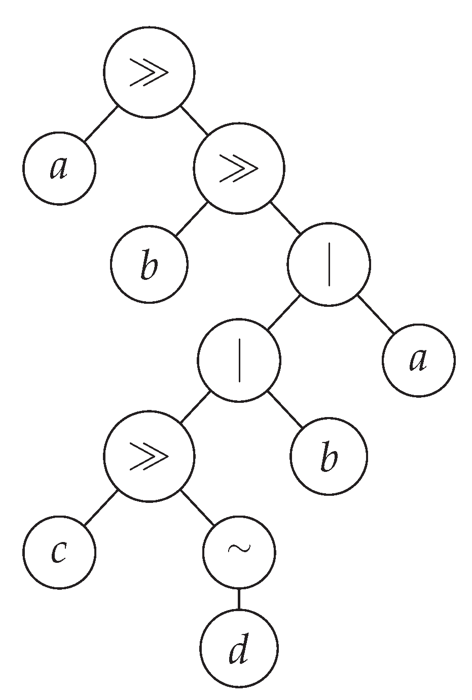
Individuals are parse trees composed of the PEG’s operators $\sim$, ≫, and |, and terminals are elements of $\mathsf{\Sigma }\cup \left\{ϵ\right\}$, where $\mathsf{\Sigma }$ is a finite alphabet (see an example in Figure 1).

An initial population is built upon $S_{+}$ (positive strings, examples) and $S_{-}$ (negative strings, counterexamples) so that each tree is consistent with a randomly chosen k-element subset, X, of $S_{+}$ and a randomly chosen k-element subset, Y, of $S_{-}$. An expression forming an individual in an initial population is created by means of a deterministic algorithm given further on. In a crossover procedure, two expressions given as parse trees are involved. A randomly chosen part of the first tree is replaced by another randomly chosen part from the second tree. The same operation is performed on the second tree in the same manner. We also used tournament selection, in which r (the tournament size) individuals are chosen at random and one of them with the highest fitness is returned. Finally, the fitness function measures an expression’s accuracy based on an individual e, and the sample $(S_{+},S_{-})$ with Equation (1):

$$f\left(t\right)=\frac{|\{w\in S_{+}:w\in L\left(G\left(e\right)\right)\}|+|\{w\in S_{-}:w\notin L\left(G\left(e\right)\right)\}|}{|S_{+}|+|S_{-}|},$$

(1)

where $G\left(e\right)$ is a non-circular PEG $G\left(e\right)=\left(\right\{A\},\mathsf{\Sigma },\{A\Leftarrow e\},A)$.

3.2. Deterministic Algorithm Used in Initializing a GP Population

For a set of strings, S, and a letter, r, by a left quotient, denoted by $r^{-1}S$, we will mean the set $\{w:rw\in S\}$, i.e., $a^{-1}\{ax,a{x}_1,x_2\}$ = $\{x,x_1\}$. Let X and Y be pairwise disjoint, nonempty sets of words over an alphabet $\mathsf{\Sigma }$. Our aim is to obtain a compact non-circular PEG G satisfying the following two conditions: (i) $X\subseteq L\left(G\right)$, (ii) $Y\cap L\left(G\right)=\varnothing$. The Algorithm 1 (function $I(X,Y)$) does it recursively.

Algorithm 1: Inferring a single expression

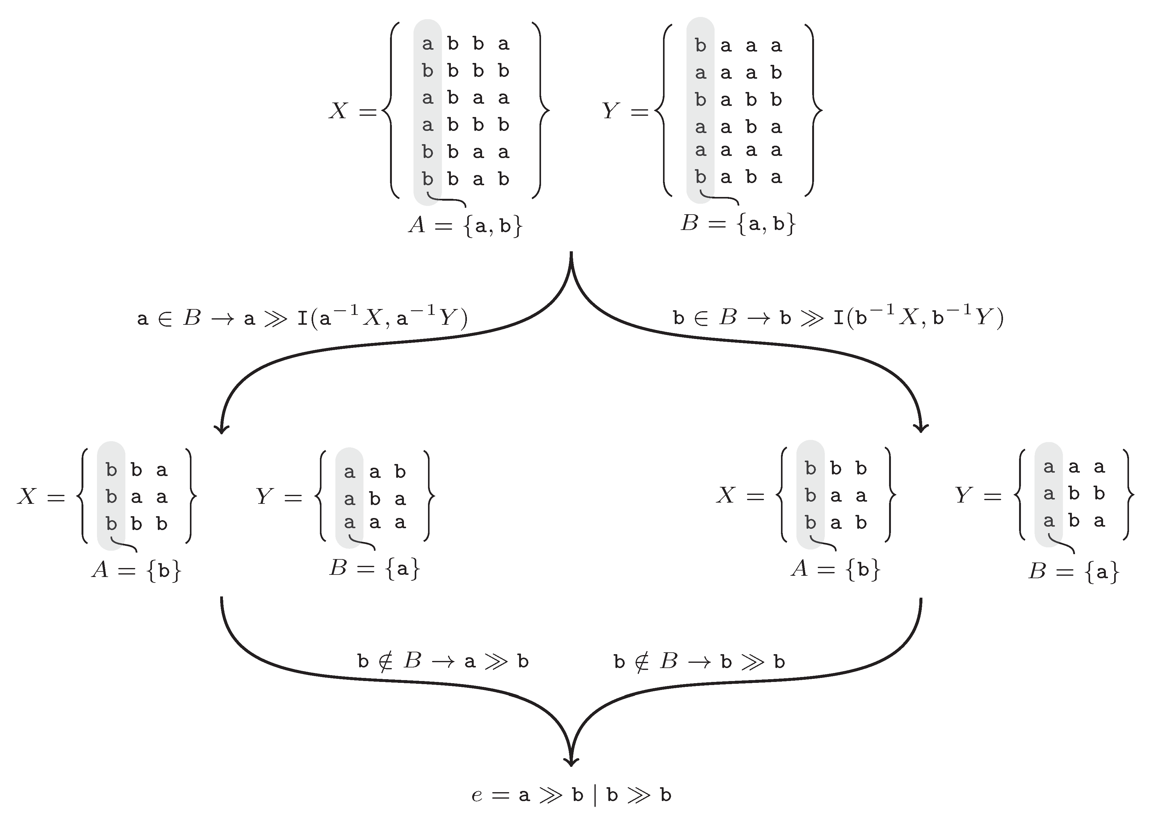
The “Append” method used in lines 7, 9, and 13 in Algorithm 1 concatenates the existing rule e with a new expression. The recursive call I in line 9 cuts sets X and Y to words that start with terminal symbol a and then all words that satisfy this condition are passed with words without the first symbol a (according to the left quotient). Line 10 is used when set A is empty. The execution of the algorithm is shown by the following example. The input is $X=\{$abba, bbbb, abaa, abbb, bbaa, bbab}, $Y=${baaa, aaab, babb, aaba, aaaa, baba}. Figure 2 shows the successive steps of the algorithm. At the beginning set, A and B are determined. The first symbols in the sets of words X, Y are equal to $\{a,b\}$. The terminal symbol a of the set A belongs to the set B. The string $a\gg$ is added to the rule e and the method is recursively invoked with left quotients $a^{-1}X$ and $a^{-1}Y$ (left leaf from the root in the Figure 2). In the next step, the a symbol is not in the set B. From the recursive call, the b symbol is returned and added to the e rule. After returning, the same procedure is repeated for the symbol b.

The algorithm has the following properties: (i) the X, Y sets in successive calls are always nonempty, (ii) word lengths can be different, (iii) it always halts after a finite number of steps and returns some PEG, (iv) the resultant PEG is consistent with X (examples) and Y (counter-examples), and (v) for random words output PEGs are many times smaller than the input. Properties from (i) to (iii) are quite obvious, (iv) will be proven, and we have checked (v) in a series of experiments, and detailed results are given in the next subsection.

Let $n=\left|X\right|+\left|Y\right|,m=\left|\mathsf{\Sigma }\right|$, the length of every word (from X and Y) not exceed d, and T be the running time of the algorithm. Then, for random input words, we can write $T(n,m,d)=O\left(n\right)+mT(n/m,m,d-1)$, which leads to $O\left(m^{min\{d,logn\}}n\right)$. In practice, m and d are small constants, so the running time of $I(X,Y)$ is usually linear with respect to n.

Lemma 1.

Let Σ be a finite alphabet and X, Y be two disjoint, finite, nonempty sets of words over Σ. If $x\in X$ and e is a parsing expression returned by $I(X,Y)$ then $\mathrm{consume}(e,x)\ne \mathrm{None}$.

Proof. 

We will prove the above by induction on k, where $k\ge 0$ is the length of x.

Basis: We use $k=0$ as the basis. Because $k=0$, $x=ϵ$. Let us consider two cases: (1) $ϵ$ is the only word in X, and (2) $\left|X\right|\ge 2$. In the first case, lines 5–9 of the algorithm are skipped and (in line 11) $e=\sim \left(a\right|b\left|c\right|\dots )$ is returned, where a, b, c, … are the first letters of Y (since $ϵ$ is in X, Y has to contain at least one nonempty word). $\mathrm{consume}(a\left|b\right|c|\dots ,ϵ)=\mathrm{None}$ implies $\mathrm{consume}(e,ϵ)=0$. In the second case, the loop in lines 5–9 and line 13 are executed, so the returned expression e (in line 14) has the following form: ${\alpha }_1\left|{\alpha }_2\right|\cdots \left|{\alpha }_j\right|\sim \left(a\right|b\left|c\right|\dots )\gg ϵ$, where ${\alpha }_i$ is a single letter, say $r_i$, or $r_i\gg {\beta }_i$ with ${\beta }_i$ being some parsing expression. For such an e, $\mathrm{consume}(e,ϵ)=0$ holds too.

Induction: Suppose that $\left|x\right|=k+1$ and that the statement of the lemma holds for all words of length j, where $0\le j\le k$. Let $x=uw$, where $u\in \mathsf{\Sigma }$. Obviously $\left|w\right|=k$. Again let us consider two cases: (1) $u\notin B$, and (2) $u\in B$. In the first case, e, which is returned in line 14, has the form $u|\alpha$ or $\alpha \left|u\right|\beta$ or $\alpha |u$, where $\alpha$ and $\beta$ are some expressions. In either case $\mathrm{consume}(e,uw)\ge 0$ (at least u will not fail for $x=uw$). In the second case, e, which is returned in line 14, is a sequence of addends, one of which is $u\gg \alpha$, where $\alpha =I(u^{-1}X,u^{-1}Y)$. Suffix w is an element of the set $u^{-1}X$ so we invoke the inductive hypothesis to claim that $\mathrm{consume}(\alpha ,w)\ne \mathrm{None}$. Then $\mathrm{consume}(e,uw)\ne \mathrm{None}$, because of the properties of the sequence and the prioritized choice operators (at least $u\gg \alpha$ will not fail for x).□

Lemma 2.

Let Σ be a finite alphabet and X, Y be two disjoint, finite, nonempty sets of words over Σ. If $y\in Y$ and e is a parsing expression returned by $I(X,Y)$ then $\mathrm{consume}(e,y)=None$.

Proof. 

We will prove the above by induction on k, where $k\ge 0$ is the length of y.

Basis: We use $k=0$ as the basis, i.e., $y=ϵ$. Because $ϵ\notin X$, the returned (in line 13) expression e has the following form: ${\alpha }_1\left|{\alpha }_2\right|\cdots |{\alpha }_j$, where ${\alpha }_i$ is a single letter, say $r_i$, or $r_i\gg {\beta }_i$ with ${\beta }_i$ being some parsing expression. For such an e, $\mathrm{consume}(e,ϵ)=\mathrm{None}$.

Induction: Suppose that $\left|y\right|=k+1$ and that the statement of the lemma holds for all words of length j, where $0\le j\le k$. Let $y=uw$, where $u\in \mathsf{\Sigma }$. Naturally $\left|w\right|=k$. There are two main cases to consider: (1) A is empty (that happens only when $X=\left\{ϵ\right\}$), and (2) A is not empty. In the first case, $e=\sim \left(a\right|b\left|c\right|\dots \left|u\right|\dots )$ is returned, where a, b, c, …, u, … are the first letters of Y (the position of u in the sequence is not important). $\mathrm{consume}(a\left|b\right|c|\dots |u|\dots ,uw)=1$ implies $\mathrm{consume}(e,y)=\mathrm{None}$. In the second case (i.e., A is not empty), let us consider four sub-cases: (2.1) $u\in A$ and $ϵ\in X$, (2.2) $u\in A$ and $ϵ\notin X$, (2.3) $u\notin A$ and $ϵ\in X$, and (2.4) $u\notin A$ and $ϵ\notin X$. As for (2.1), the returned expression e is of the following form: ${\alpha }_1\left|{\alpha }_2\right|\cdots \left|{\alpha }_j\right|\sim \left(a\right|b\left|c\right|\dots \left|u\right|\dots )\gg ϵ$, where ${\alpha }_i$ is a single letter, say $r_i$, or $r_i\gg {\beta }_i$ with ${\beta }_i$ being some parsing expression. Exactly one of ${\alpha }_i$ has the form $u\gg {\beta }_i$ (exactly one $r_i=u$), where ${\beta }_i=I(u^{-1}X,u^{-1}Y)$. Suffix w is an element of the set $u^{-1}Y$ so by the induction hypothesis $\mathrm{consume}({\beta }_i,w)=\mathrm{None}$. Then $\mathrm{consume}(e,uw)=\mathrm{None}$. Notice that the last addend—i.e., the one with $ϵ$—will also fail due to $\mathrm{consume}(\sim \left(a\right|b\left|c\right|\dots \left|u\right|\dots ),uw)=\mathrm{None}$. Sub-case (2.2) is provable similarly to (2.1). When $u\notin A$ (sub-cases 2.3 and 2.4), none of $r_i$ is u and it is easy to see that $\mathrm{consume}(e,y)=\mathrm{None}$.□

Theorem 1.

Let Σ be a finite alphabet and X, Y be two disjoint, finite, nonempty sets of words over Σ. If e is a parsing expression returned by $I(X,Y)$ and G is a non-circular PEG defined by $G=\left(\right\{A\},\mathsf{\Sigma },\{A\Leftarrow e\},A)$ then $X\subseteq L\left(G\right)$ and $Y\cap L\left(G\right)=\varnothing$.

Proof. 

This result follows immediately from the two previous Lemmas.□

3.3. Python’s PEG Library Performance Evaluation

In order to assess the fifth property of Algorithm 1 (for random words output PEGs are many times smaller than the input), we created random sets of words with different sizes, lengths and alphabets.

Table 1. The settings of the generator of random input for our PEG algorithm.

No.	$\left|\mathbf{\Sigma }\right|$	$\left|\mathit{X}\right|$	$\left|\mathit{Y}\right|$	${\mathit{d}}_{\mathbf{min}}$	${\mathit{d}}_{\mathbf{max}}$
1	2	10	10	1	10
2	2	100	100	2	20
3	4	500	500	3	30
4	4	1000	1000	4	40
5	8	5000	5000	5	50
6	8	6000	6000	6	60
7	16	7000	7000	7	70
8	16	8000	8000	8	80
9	32	9000	9000	9	90
10	32	10,000	10,000	10	100

shows our settings in this respect.

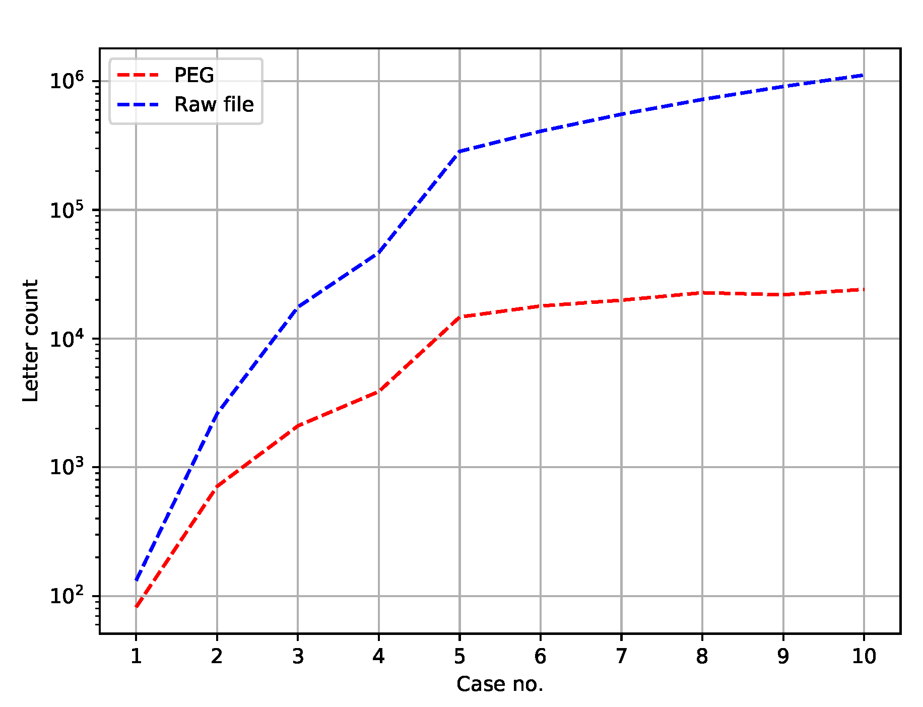
Naturally, $\left|X\right|$ and $\left|Y\right|$ denote the number of examples and counter-examples, while words’ lengths vary from $d_{max}$ to $d_{min}$. Those datasets are publicly available along with the source code of our PEG library. Figure 3 depicts the number of symbols in a PEG and the number of letters in a respective test set.

The number of letters in an input file simply equals ${\sum }_{w\in X\cup Y}\left(\left|w\right|+1\right)$, where $+1$ stands for a new line sign (i.e., words’ separator). As for PEGs, the symbol ≫ has not been counted, since it may be omitted. Outside the Python language, concatenation of two symbols, for instance a and b, can be written as $ab$ instead of $a\gg b$. Notice also that in Figure 3 the ordinates are in the logarithmic scale, because the differences are large.

The runtime of Python implementation of the proposed PEG library was benchmarked against comparable libraries, i.e., Arpeggio and Grako. The pyPEG library was rejected, because we were unable to define more complex expressions with it. As a testbed we have chosen Tomita’s languages [19]. This test set contains seven different expressions that serve as rules for the generation of words over a binary alphabet. Their description in a natural language can be found in

Table 2. PEG expressions created based on Tomita (1982) languages.

No.	Description	PEG Grammar
1	Sequence of a’s	$S\Leftarrow a\gg S\left|\sim \right(a\left|b\right)$
2	Sequence of (ab)’s	$S\Leftarrow a\gg b\gg S\left|\sim \right(a\left|b\right)$
3	Any string without an odd number of consecutive b’s after an odd number of consecutive a’s	$A\Leftarrow a\gg \sim a|a\gg a\gg A$ $B\Leftarrow b\gg \sim b|b\gg b\gg B$ $C\Leftarrow a\gg A|\sim a$ $D\Leftarrow b\gg B|\sim b$ $S\Leftarrow +(a\gg a|b)\gg S|A\gg D\gg S\left|\sim \right(a\left|b\right)$
4	Any string without more than two consecutive b’s	$S\Leftarrow (+a|ϵ)\gg (+\left(\right(b\gg b\left|b\right)\gg +a\left)\right|ϵ)\gg$ $(b\gg b\gg \sim (a\left|b\right)|b\gg \sim (a\left|b\right)\left|\sim \right(a\left|b\right))$
5	Any string of even length that, making pairs, has an even number of (ab)’s or (ba)’s	$A\Leftarrow +(a\gg a|b\gg b\left)\right|ϵ$ $B\Leftarrow a\gg b|b\gg a$ $S\Leftarrow A\gg (+(B\gg A\gg B\gg A\left)\right|ϵ)\gg A\gg \sim (a\left|b\right)$
6	Any string such that the difference between the numbers of a’s and b’s is a multiple of three	$A\Leftarrow a\gg (+(a\gg b\left)\right|ϵ)\gg (b|a\gg a)$ $B\Leftarrow b\gg (+(b\gg a\left)\right|ϵ)\gg (a|b\gg b)$ $S\Leftarrow +\left(A\right|B)\gg \sim (a\left|b\right)\left|\sim \right(a\left|b\right)$
7	Zero or more a’s followed by zero or more b’s followed by zero or more a’s followed by zero or more b’s	$A\Leftarrow +a|ϵ$ $B\Leftarrow +b|ϵ$ $S\Leftarrow A\gg B\gg A\gg B\gg \sim \left(a\right|b)$

. Seven regular expressions appropriate to the rules were created, and then the generators of random input words were implemented. Thus, for every language we had two sets: matching (positive) and non-matching (negative) words to a particular regular expression. These expressions take the following forms:

• a*
• (ab)*
• ((b|(aa))|(((a(bb))((bb)|(a(bb)))*)(aa)))*((a?)|(((a(bb))((bb)|(a(bb)))*)(a?)))
• a*((b|bb)aa*)*(b|bb|a*)
• (aa|bb)*((ba|ab)(bb|aa)*(ba|ab)(bb|aa)*)*(aa|bb)*
• ((a(ab)*(b|aa))|(b(ba)*(a|bb)))*
• a*b*a*b*

Equivalent PEG expressionswere defined as well in every comparable library (see Table 2).

Table 3. Average CPU times for available Python PEG libraries (in seconds).

Case No.	Positive/Negative	Word Length	PEG [s]	Grako [s]	Arpeggio [s]	EGG [s]
1	Positive	1–100	0.01	0.21	0.02	<0.01
1	Positive	101–1000	0.04	1.93	0.13	<0.01
1	Positive	1001–10,000	0.44	17.62	0.92	0.01
1	Positive	10,001–100,000	5.93	182	9.82	0.01
1	Negative	1–100	<0.01	0.11	0.01	0.06
1	Negative	101–1000	0.02	1.13	0.05	0.02
1	Negative	1001–10,000	0.24	9.68	0.42	–
1	Negative	10,001–100,000	2.41	81.95	3.58	–
2	Positive	1–100	0.01	0.19	0.01	<0.01
2	Positive	101–1000	0.03	1.68	0.12	<0.01
2	Positive	1001–10,000	0.12	5.64	0.4	<0.01
2	Positive	10,001–100,000	1.2	47.95	3.38	<0.01
2	Negative	1–100	<0.01	0.11	0.01	0.01
2	Negative	101–1000	0.02	0.82	0.05	0.01
2	Negative	1001–10,000	0.07	3.19	0.18	0.08
2	Negative	10,001–100,000	0.59	24.54	1.42	0.05
4	Positive	1–100	<0.01	0.2	0.02	<0.01
4	Positive	101–1000	0.04	2.12	0.36	<0.01
4	Positive	1001–10,000	0.26	12.37	2.28	<0.01
4	Positive	10,001–100,000	2.40	102.19	20.29	0.01
4	Negative	1–100	0.01	0.27	0.02	0.03
4	Negative	101–1000	0.04	2.11	0.32	0.03
4	Negative	1001–10,000	0.25	11.93	2.01	0.22
4	Negative	10,001–100,000	2.32	98.61	17.98	0.22
5	Positive	1–100	<0.01	0.2	0.02	<0.01
5	Positive	101–1000	0.04	2.12	0.36	<0.01
5	Positive	1001–10,000	0.26	12.37	2.28	0.01
5	Positive	10,001–100,000	2.4	102.19	20.29	<0.01
5	Negative	1–100	0.01	0.27	0.02	0.05
5	Negative	101–1000	0.04	2.11	0.32	0.02
5	Negative	1001–10,000	0.25	11.93	2.01	0.08
5	Negative	10,001–100,000	2.32	98.61	17.98	0.08
6	Positive	1–100	0.01	0.23	0.02	<0.01
6	Positive	101–1000	0.05	2.52	0.17	<0.01
6	Positive	1001–10,000	0.40	17.64	1.21	<0.01
6	Positive	10,001–100,000	1.67	71.70	4.93	0.01
6	Negative	1–100	0.01	0.34	0.02	0.03
6	Negative	101–1000	0.12	5.34	0.33	0.06
6	Negative	1001–10,000	1.05	44.86	2.61	0.09
6	Negative	10,001–100,000	4.61	187.90	10.42	0.17
7	Positive	1–100	<0.01	0.23	0.02	<0.01
7	Positive	101–1000	0.04	1.85	0.09	<0.01
7	Positive	1001–10,000	0.17	7.94	0.42	0.01
7	Positive	10,001–100,000	1.91	73.4	3.92	<0.01
7	Negative	1–100	<0.01	0.16	0.01	0.03
7	Negative	101–1000	0.02	1.09	0.06	0.02
7	Negative	1001–10,000	0.11	5.37	0.28	0.15
7	Negative	10,001–100,000	1.26	49.92	2.64	0.10

summarizes CPU time results. Every row contains the means for 30 runs. In all experiments we used the implementation of algorithms written in Python (our PEG library, Grako, and Arpeggio) and C++ EGG. An interpreter ran on a four-core Intel i7-965, 3.2 GHz processor in a Windows 10 operating system with 12 GB RAM.

As can be seen, in all cases our library worked much faster than other Python libraries. Grammar 3 was skipped because we were unable to define it either by means of the Arpeggio or Grako libraries. It should be stated, however, that both of the libraries have more functionality than our PEG library, its principal function being only the membership operation, i.e., matching or not a word to a PEG. As a result, Arpeggio, Grako, and pyPeg are relatively not intuitive and obvious, especially for users not familiarized with formal languages theory. The dash character in the EGG result denotes segmentation runtime error. As expected the C++ library (EGG) overcame its Python counterparts.

4. Results and Discussion

The algorithm for generating non-circular parsing expression grammars (PEG) was tested over a recently published amyloidogenic dataset [20]. The GP parameters (John Koza, a GP pioneer, has introduced a very lucid form of listing parameters in the tableau of

Table 4. Koza tableau.

Parameters	Values
Objective:	evolve expression classifying amino acid sequences according to examples and counterexamples
Terminal set:	$ϵ$, A, R, N, D, C, Q, E, G, H, I, L, K, M, F, P, S, T, W, Y, V
Function set:	$\sim$, ≫, |
Population size:	5
Crossover probability:	1.0
Selection:	Tournament selection, size $r=3$
Termination criterion:	6000 generations have passed
Maximum depth of tree after crossover:	100
Initialization method:	A special dedicated algorithm, $k=\left|X\right|=\left|Y\right|$ equals half of the cardinality of examples

named after him) are listed in Table 4. From there, we can read that a population size of $P=5$ individuals were used for GP runs along with others. The terminal set contains standard amino acid abbreviations; “A” stands for Alanine, “R” for Arginine, etc. Concerning the initialization method, see Section 3.2. The best parameters were chosen in a trial-and-error manner until the values with the best classification quality were found. The dataset is composed of 1476 strings that represent protein fragments. The data came from four databases as shown in Figure 4 and Figure 5. A total of 439 are classified as being amyloidogenic (examples), and 1037 as not (counter-examples). The shortest sequence length is 4 and the longest is 83. Such a wide range of sequence lengths was an additional impediment to learning algorithms.

In order to compare our algorithm to other grammatical inference approaches, we took most of the methods mentioned in the introductory section as a reference. Error-correcting grammatical inference [9] (ECGI) and alignment-based learning [10] (ABL) are examples of substring-based algorithms. The former builds an automaton incrementally based on the Levenstein distance between the closest word stored in the automaton and an inserted word. This process begins with an empty automaton, and for each word adds the error rules (insertion, substitution, and deletion) belonging to the transition path with the least number of error rules. The algorithm provides an automaton without loops that is more and more general. The latter, ABL, is based on searching identical and distinct parts of input words. This algorithm consists of two stages. First, all words are aligned such that it finds a shared and a distinct part of all pairs of words, suggesting that the distinct parts have the same type. For example, consider the pair “abcd” and “abe”. Here, “cd” and “e” are correctly identified as examples of the same type. The second step, which takes the same corpus as input, tries to identify the right constituents. Because the generated constituents found in the previous step might overlap, the correct ones have to be selected. Simple heuristics are used to achieve this, for example to take the constituent that was generated first (ABL-first) or to take the constituent with the highest score on some probabilistic function. We used another approach, in which all constituents are stored, but in the end we tried to keep only the minimum number of constituents that cover all examples.

ADIOS uses statistical information present in sequential data to identify significant segments and to distill rule-like regularities that support structured generalization [8]. It also brings together several crucial conceptual components; the structures it learns are (i) variable-order, (ii) hierarchically composed, (iii) context dependent, (iv) supported by a previously undocumented statistical significance criterion, and (v) dictated solely by the corpus at hand.

Blue-fringe [21] and Traxbar [22], the instances of state merging algorithms, can be downloaded from an internet archive (http://abbadingo.cs.nuim.ie/dfa-algorithms.tar.gz). They start from building a prefix tree acceptor (PTA) based on examples, and then iteratively select two states and do merging unless compatibility is broken. The difference between them comes from many ways in which the pair of states needed to merge can be chosen. Trakhtenbrot and Barzdin [23] described an algorithm for constructing the smallest deterministic FSA consistent with a complete labeled training set. The PTA is squeezed into a smaller graph by merging all pairs of states that represent compatible mappings from word suffixes to labels. This algorithm for completely labeled trees was generalized by Lang (1992) [22] to produce a (not necessarily minimum) automaton consistent with a sparsely labeled tree. Blue-fringe grows a connected set of red nodes that are known to be unique states, surrounded by a fringe of blue nodes that will either be merged with red nodes or promoted to red status. Merges only occur between red nodes and blue nodes. Blue nodes are known to be the roots of trees, which greatly simplifies the code for correct merging.

We also included one machine learning approach. An unsupervised data-driven distributed representation, called ProtVec [24], was applied and protein family classification was performed using a support vector machine classifier (SVM) [25] with the linear kernel.

The data were randomly split into two subsets, a training (75% of total) and a test set (25% of total). Given the training set and the test set, we used all algorithms to infer predictors (automata or grammars) on the training set, tested them on the test set, and computed their performances. Comparative analyses of the following five measures: Precision, Recall, F-score, the AUC, and Matthews correlation coefficient are summarized in

Table 5. Results of classification quality for the test set by the decreasing AUC.

	P	R	F1	ACC	AUC	MCC	Time [s]
PEG	0.627	0.294	0.400	0.739	0.610	0.291	0.3
ABL	0.645	0.183	0.286	0.728	0.571	0.232	412.9
ADIOS	0.329	0.633	0.433	0.508	0.544	0.082	15.6
Blue-fringe	0.367	0.303	0.332	0.639	0.541	0.088	0.9
ECGI	0.875	0.064	0.120	0.720	0.530	0.189	31.0
Traxbar	0.234	0.101	0.141	0.636	0.481	−0.05	0.3
SVM	0.224	0.001	0.131	0.526	0.471	−0.06	0.4

. The measures are given below:

• Precision, $P=\mathit{tp}/(\mathit{tp}+\mathit{fp})$;
• Recall, $R=\mathit{tp}/(\mathit{tp}+\mathit{fn})$;
• F-score, $F1=2\times P\times R/(P+R)$;
• Accuracy, $ACC=(\mathit{tp}+\mathit{tn})/(\mathit{tp}+\mathit{tn}+\mathit{fp}+\mathit{fn})$;
• Area under the ROC curve, $AUC=(\mathit{tp}/(\mathit{tp}+\mathit{fn})+\mathit{tn}/(\mathit{fp}+\mathit{tn}\left)\right)/2$;
• Matthews correlation coefficient, $\mathrm{MCC}=\frac{\mathit{tp}\times \mathit{tn}-\mathit{fp}\times \mathit{fn}}{\sqrt{(\mathit{tp}+\mathit{fp})(\mathit{tp}+\mathit{fn})(\mathit{tn}+\mathit{fp})(\mathit{tn}+\mathit{fn})}}$;
  where the terms true positives (tp), true negatives (tn), false positives (fp), and false negatives (fn) compare the results of the classifier under test with trusted external judgments. Thus, in our case, tp is the number of correctly recognized amyloids, fp is the number of nonamyloids recognized as amyloids, fn is the number of amyloids recognized as nonamyloids, and tn is the number of correctly recognized nonamyloids. The last column concerns CPU time of computations (induction plus classification in s).

The results show that there is no single method that outperformed the remaining methods regardless of an established classification measure. However, the methods can be grouped as relatively good and relatively weak from a certain angle. As regards Recall and F-score, relatively good are Blue-fringe, ADIOS, and PEG. As regards MCC, which is generally recognized as being one of the best classification measures, relatively good are PEG and ABL. Moreover, PEG achieved the best AUC, which in the case of binary prediction is equivalent to balanced accuracy.

To evaluate the convergence toward an optimal solution, we studied average fitness change over generations along with the increasing of the expression sizes (see Figure 6). The shape of the plot does not show any indication of premature convergence. Moreover, we did not observe excessive tree size expansion, which is quite often seen in genetic programming.

All programs ran on an Intel Xeon CPU E5-2650 v2, 2.6 GHz processor under an Ubuntu 16.04 operating system with 192 GB RAM. The computational complexity of all the algorithms is polynomially bounded; however, the differences in running time were quite significant and our approach ranked at the top. The algorithm for PEG induction (https://github.com/wieczorekw/wieczorekw.github.io/tree/master/PEG) was written in the Python 3 programming language. The languages of implementation for six successive methods were: Python, Java, C, Python, C, and Python.

5. Conclusions

We proposed a new grammatical inference (PEG-based) method and applied it to a real bioinformatics task, i.e., classification of amyloidogenic sequences. The evaluation of generated PEGs on an amyloidogenic dataset revealed the method’s accuracy in predicting amyloid segments. We showed that the new grammatical inference algorithm gives the best ACC, AUC, and MCC scores in comparison to five other automata or grammar learning methods and the ProtVec/SVM method.

In the future, we will implement circular rules in the PEG library, which will improve the expressiveness of grammars and may improve the quality of classification.

References

- De la Higuera, C. Grammatical Inference: Learning Automata and Grammars; Cambridge University Press: New York, NY, USA, 2010. [Google Scholar]
- Wieczorek, W. Grammatical Inference—Algorithms, Routines and Applications; Studies in Computational Intelligence; Springer: Cham, Switzerland, 2017; Volume 673. [Google Scholar] [CrossRef]
- Gold, E.M. Language Identification in the Limit. Inf. Control 1967, 10, 447–474. [Google Scholar] [CrossRef] [Green Version]
- Coste, F.; Fredouille, D. Unambiguous Automata Inference by Means of State-Merging Methods. In Proceedings of the Machine Learning: ECML 2003, 14th European Conference on Machine Learning, Cavtat-Dubrovnik, Croatia, 22–26 September 2003; pp. 60–71. [Google Scholar]
- Miclet, L. Grammatical Inference. In Syntactic and Structural Pattern Recognition Theory and Applications; Bunke, H., Sanfeliu, A., Eds.; World Scientific Series in Computer Science; World Scientific: Singapore, 1990; Volume 7, pp. 237–290. [Google Scholar]
- Dupont, P. Regular grammatical inference from positive and negative samples by genetic search: The GIG method. In Grammatical Inference and Applications; Carrasco, R.C., Oncina, J., Eds.; Springer: Berlin/Heidelberg, Germany, 1994; pp. 236–245. [Google Scholar]
- Sakakibara, Y. Learning context-free grammars using tabular representations. Pattern Recognit. 2005, 38, 1372–1383. [Google Scholar] [CrossRef]
- Solan, Z.; Horn, D.; Ruppin, E.; Edelman, S. Unsupervised learning of natural languages. Proc. Natl. Acad. Sci. USA 2005, 102, 11629–11634. [Google Scholar] [CrossRef] [PubMed] [Green Version]
- Rulot, H.; Vidal, E. Modelling (Sub)String Length Based Constraints through a Grammatical Inference Method. In Proceedings of the NATO Advanced Study Institute on Pattern Recognition Theory and Applications; Devijver, P.A., Kittler, J., Eds.; Springer: Berlin/Heidelberg, Germany, 1987; pp. 451–459. [Google Scholar]
- van Zaanen, M. ABL: Alignment-based Learning. In Proceedings of the 18th Conference on Computational Linguistics—Volume 2, Jcken, Germany, 31 July–4 August 2000; Association for Computational Linguistics: Stroudsburg, PA, USA, 2000. COLING ’00. pp. 961–967. [Google Scholar] [CrossRef]
- Eyraud, R.; de la Higuera, C.; Janodet, J.C. LARS: A learning algorithm for rewriting systems. Mach. Learn. 2007, 66, 7–31. [Google Scholar] [CrossRef] [Green Version]
- Kuramitsu, K.; ya Hamaguchi, S. XML schema validation using parsing expression grammars. PeerJ Prepr. 2015, 3, e1503. [Google Scholar]
- Ierusalimschy, R. A text pattern-matching tool based on Parsing Expression Grammars. Softw. Pract. Exp. 2009, 39, 221–258. [Google Scholar] [CrossRef] [Green Version]
- Moss, A. Simplified Parsing Expression Derivatives. In Language and Automata Theory and Applications; Leporati, A., Martín-Vide, C., Shapira, D., Zandron, C., Eds.; Springer International Publishing: Cham, Switzerland, 2020; pp. 425–436. [Google Scholar]
- Hopcroft, J.E.; Motwani, R.; Ullman, J.D. Introduction to Automata Theory, Languages, and Computation, 2nd ed.; Addison-Wesley Longman Publishing Co., Inc.: Boston, MA, USA, 2001. [Google Scholar]
- Ford, B. Parsing expression grammars: A recognition-based syntactic foundation. In Proceedings of the 31st ACM SIGACT/SIGPLAN Symposium on Principles of Programming Languages, Venice, Italy, 14–16 January 2004; Volume 39, pp. 111–122. [Google Scholar]
- Grune, D.; Jacobs, C. Parsing Techniques: A Practical Guide; Springer: New York, NY, USA, 2008; pp. 1–662. [Google Scholar] [CrossRef]
- Banzhaf, W.; Francone, F.D.; Keller, R.E.; Nordin, P. Genetic Programming: An Introduction: On the Automatic Evolution of Computer Programs and Its Applications; Morgan Kaufmann Publishers Inc.: San Francisco, CA, USA, 1998. [Google Scholar]
- Tomita, M. Learning of Construction of Finite Automata from Examples Using Hill-Climbing: RR: Regular Set Recognizer; Department of Computer Science, Carnegie-Mellon University: Pittsburgh, PA, USA, 1982. [Google Scholar]
- Wozniak, P.; Kotulska, M. AmyLoad: Website dedicated to amyloidogenic protein fragments. Bioinformatics 2015, 31, 3395–3397. [Google Scholar] [CrossRef] [PubMed] [Green Version]
- Lang, K.; Pearlmutter, B.; Price, R. Results of the Abbadingo one DFA Learning Competition and a New Evidence-Driven State Merging Algorithm; Lecture Notes in Computer Science (Including Subseries Lecture Notes in Artificial Intelligence and Lecture Notes in Bioinformatics); Springer: Berlin/Heidelberg, Germany, 1998; Volume 1433, pp. 1–12. [Google Scholar]
- Lang, K.J. Random DFA’s can be approximately learned from sparse uniform examples. In Proceedings of the Fifth Annual ACM Workshop on Computational Learning Theory, Pittsburgh, PA, USA, 27–29 July 1992; ACM: New York, NY, USA; Pittsburgh, PA, USA, 1992; pp. 45–52. [Google Scholar]
- Trakhtenbrot, B.; Barzdin, Y. Finite Automata: Behavior and Synthesis; Fundamental Studies in Computer Science; North-Holland Publishing Company: Amsterdam, The Netherlands, 1973. [Google Scholar]
- Asgari, E.; Mofrad, M.R.K. Continuous Distributed Representation of Biological Sequences for Deep Proteomics and Genomics. PLoS ONE 2015, 10, 1–15. [Google Scholar] [CrossRef] [PubMed]
- Wu, T.F.; Lin, C.J.; Weng, R.C. Probability Estimates for Multi-class Classification by Pairwise Coupling. J. Mach. Learn. Res. 2004, 5, 975–1005. [Google Scholar]
Figure 1.
Example of a genetic programming individual coded as the expression a≫b≫ (c≫∼d|b|a).
Figure 2.
Example of the proposed Induction algorithm.
Figure 3.
The number of symbols in a PEG (red line) and the number of letters in a respective test set (blue line).
Figure 4.
Combined amyloid databases used in this work. Pos and Neg denote, respectively, positive and negative word counts in the database.
Figure 5.
Combined amyloid databases used in work. Pos and Neg denote, respectively, positive and negative word counts in the database.
Figure 6.
Average error (fitness accuracy) vs. expression length for different generations based on random data with two letters in the alphabet, 100 words at each set of example and counter-example and word lengths between 2 and 20.