Superpixel-Based Regional-Scale Grassland Community Classification Using Genetic Programming with Sentinel-1 SAR and Sentinel-2 Multispectral Images

Abstract

Grasslands are one of the most important terrestrial ecosystems on the planet and have significant economic and ecological value. Accurate and rapid discrimination of grassland communities is critical to the conservation and utilization of grassland resources. Previous studies that explored grassland communities were mainly based on field surveys or airborne hyperspectral and high-resolution imagery. Limited by workload and cost, these methods are typically suitable for small areas. Spaceborne mid-resolution RS images (e.g., Sentinel, Landsat) have been widely used for large-scale vegetation observations owing to their large swath width. However, there still keep challenges in accurately distinguishing between different grassland communities using these images because of the strong spectral similarity of different communities and the suboptimal performance of models used for classification. To address this issue, this paper proposed a superpixel-based grassland community classification method using Genetic Programming (GP)-optimized classification model with Sentinel-2 multispectral bands, their derived vegetation indices (VIs) and textural features, and Sentinel-1 Synthetic Aperture Radar (SAR) bands and the derived textural features. The proposed method was evaluated in the Siziwang grassland of China. Our results showed that the addition of VIs and textures, as well as the use of GP-optimized classification models, can significantly contribute to distinguishing grassland communities, and the proposed approach classified the seven communities in Siziwang grassland with an overall accuracy of 84.21% and a kappa coefficient of 0.81. We concluded that the classification method proposed in this paper is capable of distinguishing grassland communities with high accuracy at a regional scale.

1. Introduction

As the largest terrestrial ecosystem on earth, grasslands play a crucial role in regulating climate, conserving water, protecting biodiversity, and promoting livestock development [1,2]. Grassland communities are considered the fundamental unit of grassland ecosystems [3]. Accurate classification of grassland communities is important for humans to understand and study grassland areas, and provides an important basis for rational use, effective conservation, and sustainable development [4]. Field surveys are a reliable way to classify grasslands. Researchers can obtain accurate information on the distribution of different grasslands through sampling and obtaining field records. However, this method is costly and time-consuming when applied either repetitively or in large landscapes [5].

Remote sensing (RS) technology developed through advances in aerospace technology, provides a method for achieving fast, effective and objective observation of grasslands [6]. Each pixel in the image is classified into different categories based on certain rules through extraction of the spectral, textural, and spatial features of different categories of grassland from RS images [7]. Recently, unmanned aerial vehicle (UAV) images were widely used in grassland community classification due as they are characterized by less restrictive weather conditions and low cost of operation [8,9]. However, the low altitude of UAVs results in more time required to photograph large areas of grassland. Therefore, the study area for grassland community classification studies based on UAV data is typically a few tens to a few hundred square kilometers [10,11,12].

Spaceborne mid-resolution RS images (e.g., GaoFen-6, Sentinel-2, Landsat-8) have larger swath width, thus they are more suitable for large-scale studies [13,14]. However, studies using these images for classifying grassland at community level are rare [15]. One reason for this can be attributed to the low spectral resolution of these images, which causes the spectral differences between different communities to be insignificant and thus makes it difficult to distinguish them using raw multispectral images alone [7,16]. Recent studies have attempted vegetation classification using vegetation indices (VIs) reflecting vegetation growth status [17] and textural features reflecting image homogeneity [18] in combination with raw multispectral images and have succeeded in improving vegetation classification [19]. In addition, spaceborne synthetic aperture radar (SAR) data has been found to discriminate vegetation types well due to its all-weather acquisition capability [20]. Also, several studies have shown that the fused multispectral and SAR imagery has a better performance than using a single type of data in vegetation mapping [21]. And in these studies, Sentinel-1 SAR and -2 multispectral data are commonly used. This implies the potential of Sentinel satellite data, the outcomes of the European Copernicus program, in grassland community classification [5].

The other reason for the difficulty in distinguishing grassland communities using spaceborne mid-resolution RS images is that the performance of the classification models used to classify grassland communities is suboptimal [3]. In previous studies of vegetation classification, classification models (including classifiers and their hyperparameters) were usually determined empirically without selecting the optimal ones based on the specific study [22,23]. Notably, studies suggest that the selection of classification models has a significant impact on the classification results [24,25]. The advanced Genetic Programming (GP) algorithm which is a type of Genetic Algorithm (GA) [26], has been recently used in the field of model optimization [27]. GP automatically searches for optimal solutions to problems by simulating natural biological evolutionary mechanisms. GP can optimize both classifiers and hyperparameters [28] as opposed to the common optimization methods such as grid search, random search, and Bayesian optimization. Moreover, it can generate more complex models to achieve higher accuracy when faced with complicated prediction problems [29].

As for the basic unit of classification, superpixels composed of spatially connected similar pixels can adhere better to the natural image boundaries compared with pixels [30]. Therefore, the superpixel-based classification results can alleviate the salt-and-pepper phenomenon and obtain better classification results compared to pixel-based [31]. Moreover, the computational burden of superpixel-based classification is small, and the result is less affected by noise [32], thus the studies of RS vegetation classification are commonly conducted with superpixels as the basic unit [33].

In this study, we aimed to propose a superpixel-based regional-scale grassland community classification method using the GP-optimized classification model with Sentinel-2 multispectral bands, their derived VIs and textures, and Sentinel-1 SAR bands and the derived textures. The method was validated in Siziwang grassland, China. The objectives of the study were to: (1) verify whether the addition of textures and VIs would improve the classification accuracy of grassland communities based on spaceborne mid-resolution RS images; (2) test whether the classification results based on the GP-optimized classification model are better than that of common classifiers; (3) map the distribution of Siziwang grassland communities; (4) evaluate the universality of the proposed method. We expected that the method proposed in this paper can achieve high accuracy classification of grassland communities based on spaceborne mid-resolution RS data at a regional scale with high universality.

2. Study Area and Data

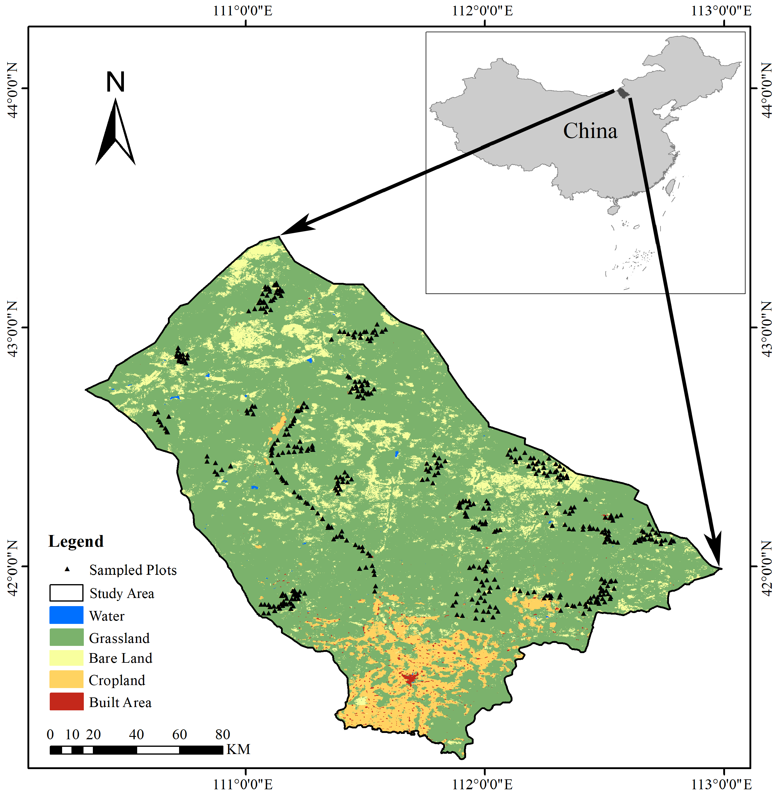
2.1. Study Area

Siziwang Banner (Figure 1) is part of Ulanqab city in Inner Mongolia, China. It is located in the central part of Inner Mongolia, at a latitude/longitude of 41.17° to 43.37° N, 110.33° to 113° E, and covers an area of 24,036 km² [34]. The region is situated at the northern foot of Daqing Mountain, with an altitude of 1000 to 2100 m, and the entire terrain is inclined from southeast to northwest. Siziwang Banner is characterized by a mid-temperate continental monsoon climatic zone, with an average annual rainfall of 310.2 mm, and 70% of the yearly precipitation occurs mainly in July, August, and September. The average annual temperature of the region is 3.8 °C with the lowest temperature recorded in January (−17.2 °C) and the highest temperature recorded in July (20.7 °C) [35]. Occupying approximately 80% of the total area of Siziwang, Siziwang grassland is an important part of the grasslands in northern China and the Eurasian grassland [34]. The main communities here (

Table 1. Main grassland communities in Siziwang.

Community	Constructive Species [36]	Coverage (%) [36]	Examples
RES	Reaumuria soongarica (Pall.) Maxim	8–12
STC	Stipa caucasica subsp. glareosa (P. A. Smirn.) Tzvelev	10–15
STT	Stipa tianschanica var. gobica (Roshev.) P. C. Kuo & Y. H. Sun	10–20
ARF	Artemisia frigida willd	20–25
STB	Stipa breviflora Griseb	20–40
STS	Stipa sareptana var. krylovii (Roshev.) P. C. Kuo & Y. H. Sun	35–40
ACS	Achnatherum splendens (Trin.) Nevski	35–50

) include Reaumuria soongarica (Pall.) Maxim (hereafter RES) grassland, Stipa sareptana var. krylovii (Roshev.) P. C. Kuo & Y. H. Sun (hereafter STS) grassland, Artemisia frigida willd (hereafter ARF) grassland, Stipa tianschanica var. gobica (Roshev.) P. C. Kuo & Y. H. Sun (hereafter STT) grassland, Stipa caucasica subsp. glareosa (P. A. Smirn.) Tzvelev (hereafter STC) grassland, Stipa breviflora Griseb (hereafter STB) grassland, and Achnatherum splendens (Trin.) Nevski (hereafter ACS) grassland [36].

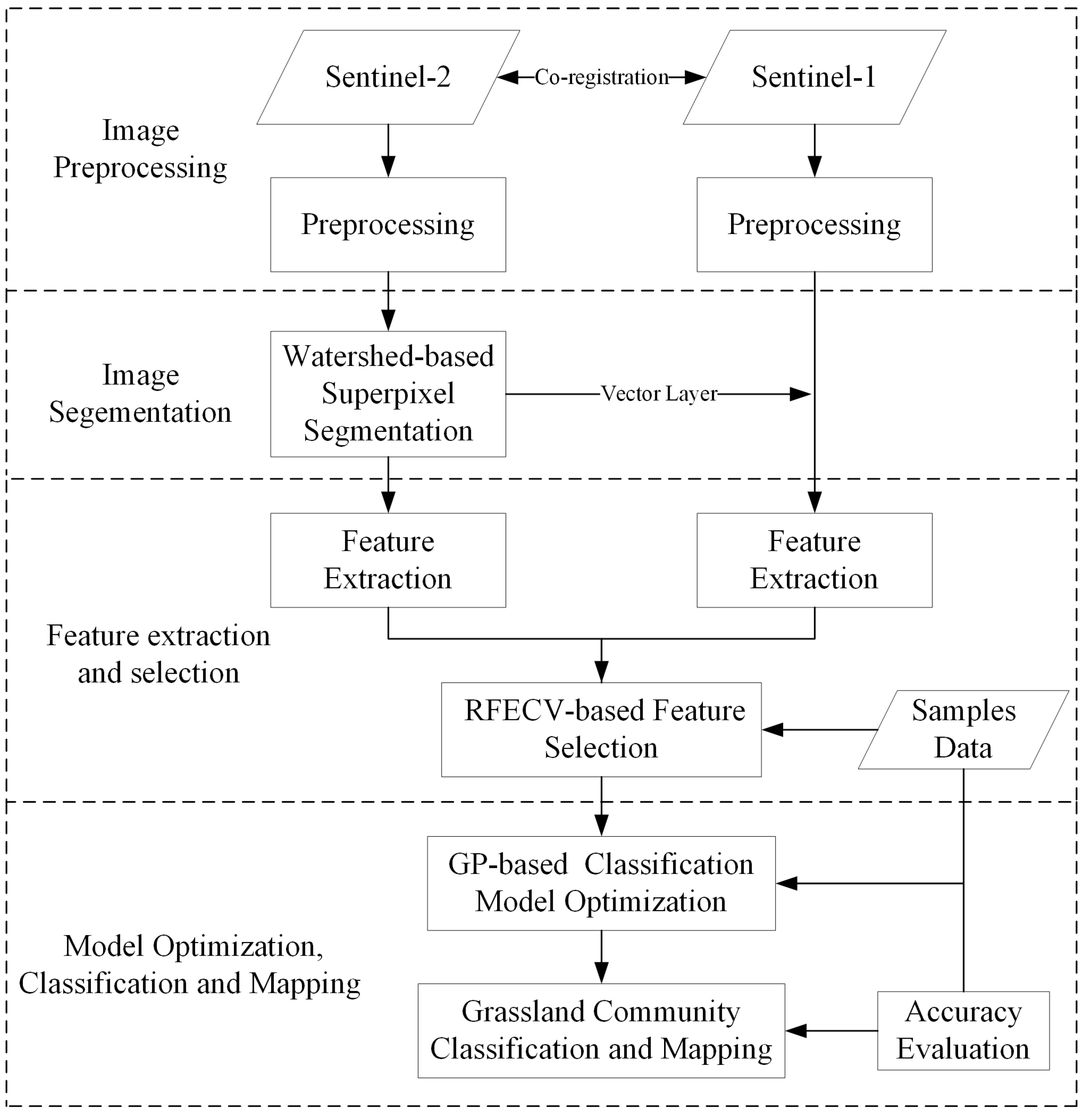
2.2. Image Preprocessing

Sentinel-1 and Sentinel-2 are sensors developed by the European Space Agency (ESA) Copernicus for earth observation. The sensors are commonly used in vegetation studies owing to the high data quality and availability [4,38]. The Sentinel images used in this study (

Table 2. Basic information of the Sentinel data used in this study.

Satellite	Acquisition Time	Product Type	Number of Images	Cloud Percentage
Sentinel-1	2 July 2019, 7 July 2019	GRD	4	—
Sentinel-2	3 July 2019	Level-2A	7	Less than 1%

) were retrieved from Sentinels Scientific Data Hub (https://scihub.copernicus.eu/, accessed on 1 August 2020), resampled to 10 m using bilinear interpolation, geographically registered, and subset into the study area.

2.2.1. Sentinel-1 Data

Sentinel-1 carries a C-band SAR with a 6-day repeat cycle [39]. Sentinel-1 data used in this study were Level-1 Ground Range Detected (GRD) images in Interferometric Wide Swath (IW) mode at VV (vertical transmit and vertical receive) and VH (vertical transmit and horizontal receive) polarizations with 250 km swath width and 5 m × 20 m spatial resolution [40]. The preprocessing of Sentinel-1 GRD data included applying orbit file, border and thermal noise removal, radiometric calibration, speckle filtering, range doppler terrain correction, and geocoding [41]. Preprocessing was conducted using an open-source SNAP software (version 8.0.0) (https://step.esa.int/main/toolboxes/snap/, accessed on 7 May 2020) and obtained higher quality GRD data for the subsequent experiments.

2.2.2. Sentinel-2 Data

Sentinel-2 comprises two satellites with a revisit period of 5 day and a swath width of 290 km. Sentinel-2 Multispectral Instrument (MSI) covers 13 spectral bands from visible to short-wave infrared (SWIR) (

Table 3. Sentinel-2 band information [44].

Sentinel-2 Bands	Central Wavelength ($\mathsf{\mu }$m)	Spatial Resolution (m)
Band 1: Coastal aerosol	0.443	60
Band 2: Blue	0.490	10
Band 3: Green	0.560	10
Band 4: Red	0.665	10
Band 5: Vegetation red edge	0.705	20
Band 6: Vegetation red edge	0.740	20
Band 7: Vegetation red edge	0.783	20
Band 8: NIR	0.842	10
Band 8b: Narrow NIR	0.865	20
Band 9: Water vapour	0.945	60
Band 10: SWIR-Cirrius	1.375	60
Band 11: SWIR	1.610	60
Band 12: SWIR	2.190	60

), including 4 bands in the red, green, blue, and near-infrared (NIR) region with a spatial resolution of up to 10 $\mathrm{m}$, which is currently the highest multispectral data freely available [42]. Moreover, Sentinel-2 Level-2A data has been orthographic, atmospheric, geometric corrected [43].

2.3. Ground Truth Data Acquisition

The field survey was conducted in August 2019. It should be noted that the proposed approach used superpixels as the basic unit of classification, implying that the samples used for classification were obtained by assigning observations of the community categories to the superpixels where the sampling points were located. Therefore, field sampling was conducted in patches with a homogeneous grassland community, and the locations of field points were recorded by GPS. In addition to field sampling, more samples were selected for classification based on previous studies [36,45]. A total of 378 field sites with RES (45 sites), STC (41 sites), STT (67 sites), ARF (30 sites), STB (44 sites), STS (72 sites), and ACS (79 sites) were included in the current study. Of these, 70% were used for training the classification model and 30% were used for testing the classification accuracy. Considering no significant changes in the extend of the grassland in Siziwang Banner between 2019 to 2020 [34,37], we masked off non-grassland areas to eliminate their interference of the classification results using the 10 $\mathrm{m}$ resolution Siziwang Banner land cover map for 2020 [37].

3. Methods

The flow chart of the proposed classification method of grassland community is summarized in Figure 2. The method consists of four parts, including the part of image processing which is introduced in Section 2.2, and the other three parts are discussed in detail in this section.

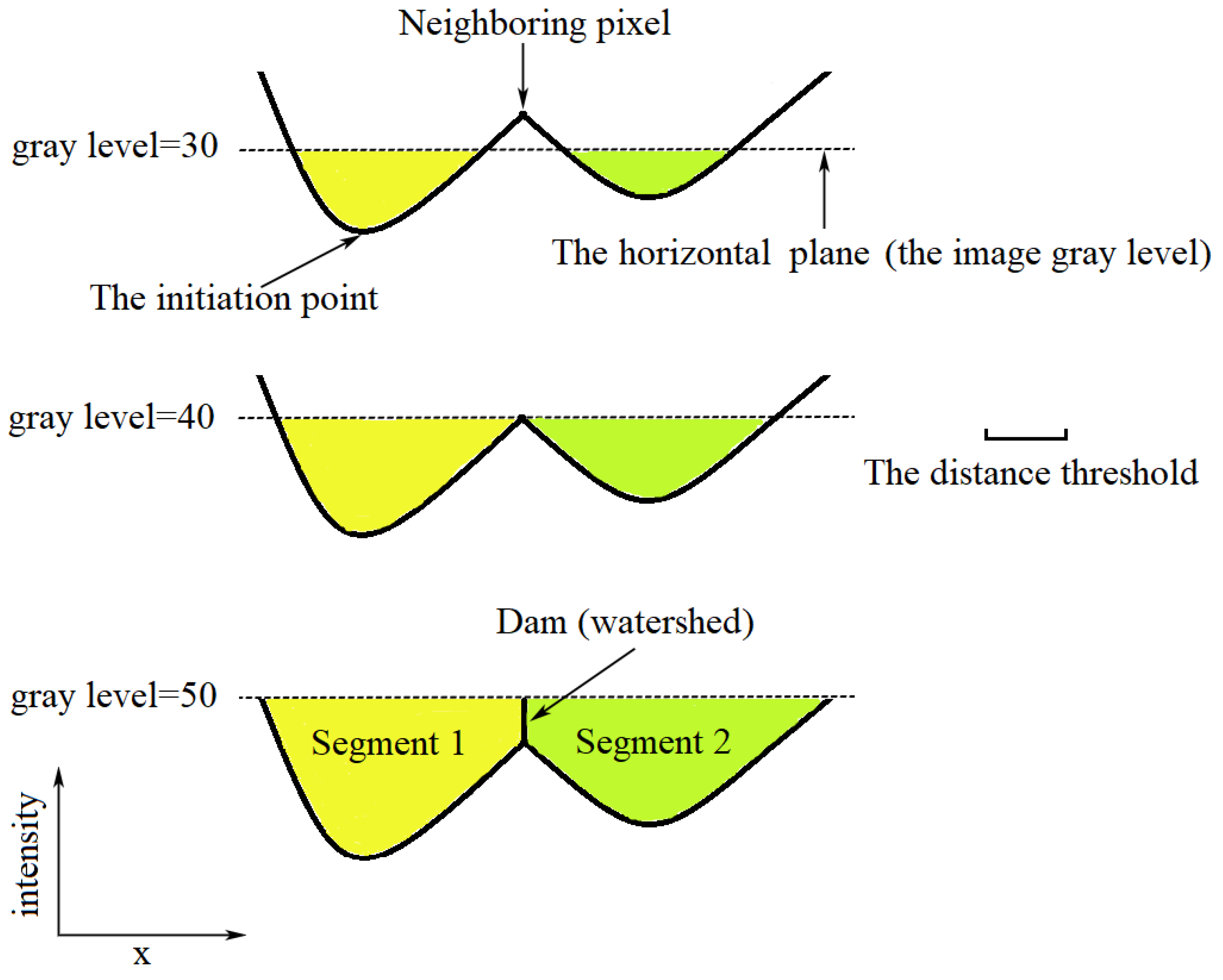
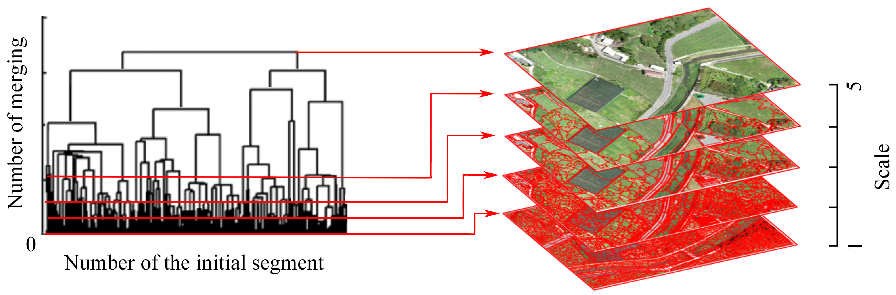
3.1. Watershed-Based Superpixel Segmentation

The watershed algorithm is a segmentation method based on analysis of geomorphology and is widely used in RS image processing [46,47]. The algorithm achieves image segmentation by connecting pixels with similar features (usually refers to gray values) to each other in spatial location thus forming a closed contour. Specifically, at first, the gray value of all pixels in an image is extracted and a distance threshold is set. Then, taking the pixel with the smallest gray value as the initiation point, the horizontal plane (i.e., the image gray level) raises from the minimum gray value. When the horizontal plane reaches the neighboring pixels, the horizontal distance from these pixels to the initiation point is calculated, and if it is less than the threshold distance, these pixels are flooded (implying that they are included as pixels inside the segmented object), otherwise dams (i.e., watersheds) are set on these pixels to segment these neighboring pixels. Increase in the horizontal plane then more dams are set, and when the horizontal plane reaches the maximum of gray value, these dams complete the segmentation of the whole image [48]. The process of watershed segmentation is presented in Figure 3.

It is worth noting that setting of the distance threshold has a significant effect on the results of segmentation and classification [49]. A large threshold leads to inclusion of heterogeneous pixels within the segmented object, whereas a small threshold results in inadequate image segmentation. The stepwise evolution analysis (SEA) method proposed by Hu et al. (2017) [50] was used in the current study to obtain the optimal segmentation scale. The first step of SEA is to construct the scale set model [51] that records the image segmentation results at each scale on the already segmented images. Concretely, the neighboring segments are merged pairwise in descending order of dissimilarity, and binary segmentation trees [52] are used to record the new segments created during the merging process and the hierarchical relationships between all child segments and parent segments. When the merging is completed, the scale set model of the image is built. An example of a scale set model is shown in Figure 4. The larger the segmentation scale is, the more under-segmentation exists; conversely, the more over-segmentation exists. Subsequently, SEA solves for the optimal segmentation scale by evaluating the risk of over- and under-segmentation at each scale using the minimum risk Bayesian decision algorithm [53]. The performance of this method has been confirmed in several studies [54,55,56]. It is worth noting that since speckle noise in SAR data would interfere with the performance of segmentation [57,58], we only performed segmentation on multispectral data. Then, the segmented vector layer was applied to SAR data to segment it.

3.2. Feature Extraction and Selection

Four categories of features derived from Sentinel-1 and -2 were utilized in this study, including spectral information, VIs, textural features, and backscatter information (

Table 4. Description of features extracted from Sentinel-1 and 2 images.

Categories	Features	Description	Reference
Spectral Information	Band 2, 3, 4, 5, 6, 7, 8, and 8b	The reflectance in red, blue, green, NIR, and red edge band	[42]
Vegetation Indices	NDVI	$\frac{{\rho }_{nir}-{\rho }_{red}}{{\rho }_{mir}+{\rho }_{red}}$	[60]
	SR	$\frac{{\rho }_{nir}}{{\rho }_{red}}$	[60]
	EVI	$2.5\times \frac{{\rho }_{nir}-{\rho }_{red}}{{\rho }_{nir}+6\times {\rho }_{red}-7.5\times {\rho }_{blue}+1}$	[61]
	$NDV{I}_{705}$	$\frac{{\rho }_{750}-{\rho }_{705}}{{\rho }_{750}+{\rho }_{705}}$	[62]
Textural Features	GLGM_Variance, GLGM_Homogeneity, GLGM_Contrast, GLGM_Dissimilarity, GLGM_Entropy, GLGM_Correlation, GLGM_Second Moment	Variance, Homogeneity, Contrast, Dissimilarity, Entropy, Correlation, and Second Moment of VV and VH polarization	[63]
Backscatter Information	${\sigma }_{VV}$ and ${\sigma }_{VH}$	Backscatter coefficient of VV and VH polarization	[39]

${\rho }_{nir}$, ${\rho }_{red}$, ${\rho }_{blue}$, ${\rho }_{705}$, and ${\rho }_{750}$ represent NIR, red, blue, red edge 1, and red edge 2 band of Sentinel-2, respectively.

). VIs included NDVI, Enhanced Vegetation Index (EVI), Simple Ratio Index (SR), and Red Edge Normalized Difference Vegetation Index ($NDV{I}_{705}$). The textural features used in this study were derived from the gray-level co-occurrence matrix (GLCM), and seven GLCM indicators of two backscatter coefficients and eight spectral bands were calculated with a window size of $9\times 9$, which has been reported by several studies as suitable for extracting textures from Sentinel images [38,59]. The abovementioned features were calculated from SNAP software at the pixel level. For each superpixel, the mean and standard deviation of these features were computed.

Notably, not all the extracted features contribute to improving the classification accuracy [64]. Therefore, several feature selection algorithms have been proposed to eliminate the effects of noisy data on classification results. The Recursive Feature Elimination with Cross-Validation (RFECV) algorithm is widely used in image analysis for automatic selection of the optimal feature subset without human intervention [18]. RFECV first ranks the features in order of importance and then selects the optimal feature subset by cross-validation [65]. The above two processes are specifically as follows.

• N features are fed into a classifier, and importance of each feature is calculated;
• The feature with the lowest importance is removed from the current feature set, and the other features are input into the classifier again to calculate importance of each feature;
• Step 2 is repeated until the feature set was empty;
• All features are sorted by decreasing order of importance, and a threshold is selected. The features with importance greater than this threshold are then retained.

In previous studies, the threshold was usually determined by repeated experiments [18]. To capture the optimal feature subset automatically, the RFE with cross-validation (RFECV) algorithm was employed in this study. RFECV used the classifier in RFE to calculate the validation error of all feature subsets ($2^n-1$) consisting of n features, and the number of features in the subset with the lowest average validation error was the optimal number of features. The optimal features were then selected based on the ranking obtained by RFE [66]. Since RF excels in feature selection and ranking [67], it was chosen as the classifier of RFE (hereafter RF_RFE) in this study.

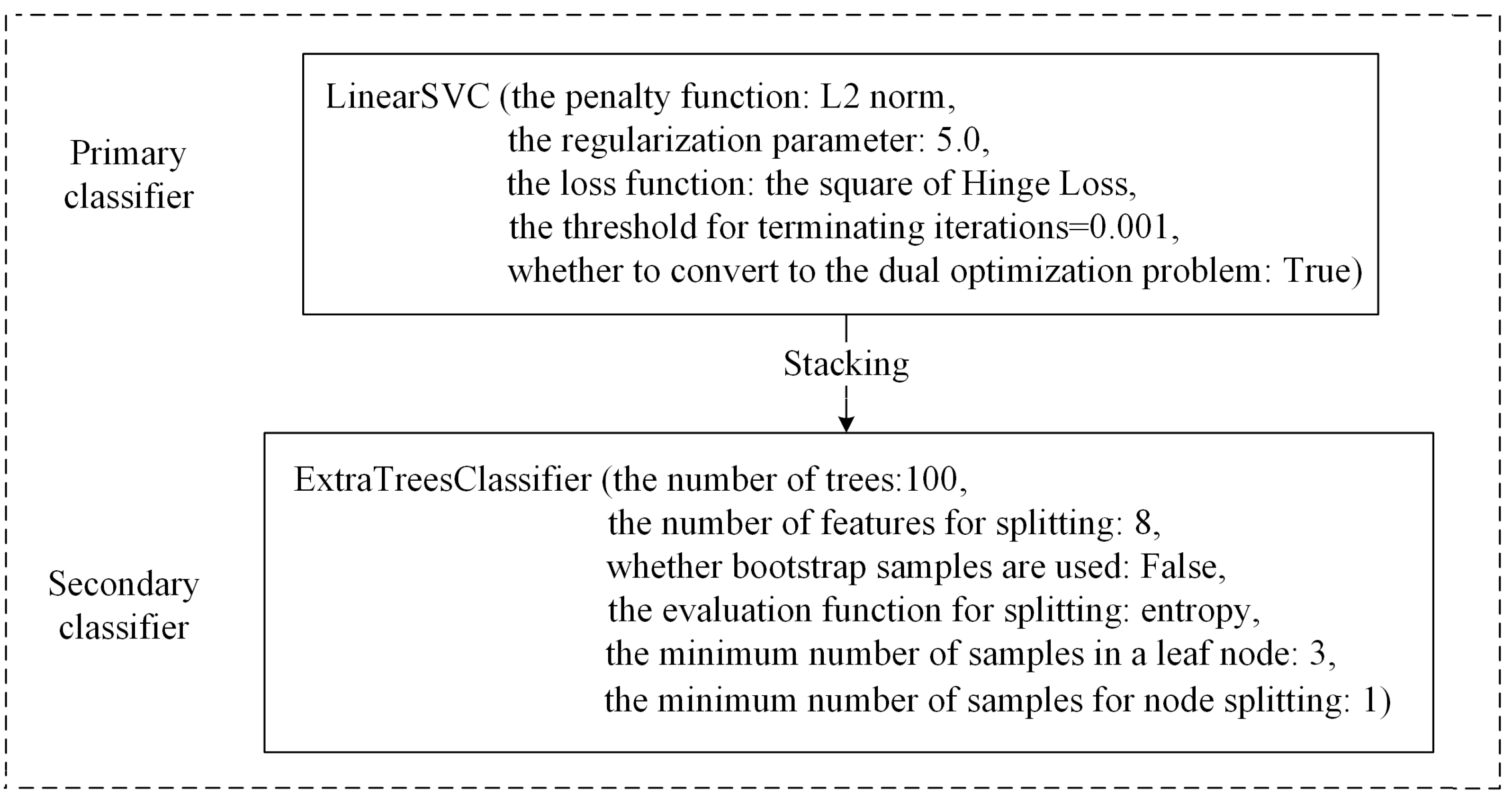
3.3. Classification Selection and Hyperparameter Optimization Based on GP Algorithm

The GP algorithm is a search and optimization technique that simulates the process of Darwinian biological evolution [68]. It expresses the feasible solutions for the problem by using individuals. The initial population evolves to the optimal individual tree, i.e., the optimal solution, for the solution problem after genetic operations such as replication, crossover, and mutation, guided by the fitness function.

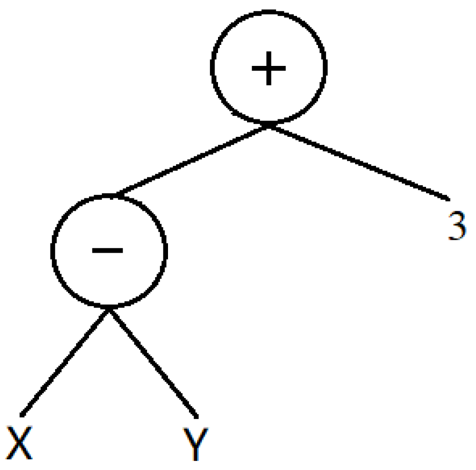
3.3.1. Individual Tree

GP is an evolutionary algorithm, which inherits the Genetic algorithm’s (GA) idea of breeding offspring from parents by selection. However, unlike the traditional coding (fixed-length gene) model of GA, individuals in GP are represented in a hierarchical structure instead of a string, most often in a tree structure [69].

The individual tree comprises the terminal set (TS) and function set (FS), whereby TS and FS hold the input variables and the functions that perform operations on the input variables, respectively. Figure 5 shows an individual tree expressing $(X-Y)+3$, where the functions (+, −) on the internal nodes and the variables (X, Y, 3) on the leaf nodes are generated from FS and TS, respectively. In this study, GP was performed using the scikit-learn, xgboost, TPOT, and DEAP packages in Python. TS comprises the superpixels awaiting classification and samples. FS comprises the classification models in the sklearn machine learning Python package, including Logistic Regression (LR), Stochastic Gradient Descent (SGD), K-nearest neighbor (KNN), Decision Tree (DT), Naive Bayes (NB), Support Vector Machine (SVM), Linear Discriminant Analysis (LDA), Quadratic Discriminant Analysis (QDA), Bagging, Random Forest (RF), AdaBoost, Extremely Randomized Trees (ET), Gradient Tree Boosting (GBDT) and Multilayer Perception (MLP), etc.

3.3.2. Genetic Operator

GP contains three genetic operators: replication, crossover, and mutation. The structure of individual trees can change when new trees are generated owing to the genetic operators.

• The replication operator selects a few individuals in the current population according to certain rules and retains them directly to the next generation.
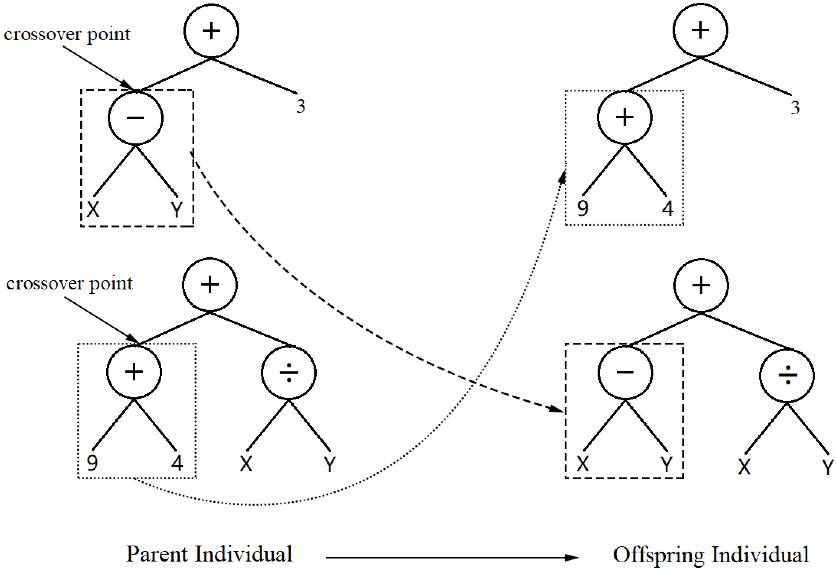
• The crossover operator randomly selects two individuals as parents from the current population. A node is then randomly selected as the crossover point in each parent individual, and the part below this node represents the segment to be exchanged (called the crossover segment). Offspring individuals are generated by swapping the crossing segments of parent individuals. The crossover process of individual trees $(X-Y)+3$ and $(9+4)+(X÷Y)$ is presented in Figure 6.
• The mutation operator randomly selects a node in a parent individual as a mutation point and replaces the subtree below the mutation point with a randomly generated individual tree. Figure 7 illustrates the mutation process of the individual tree $(X-Y)+3$.

3.3.3. Fitness Function

After individuals are generated, it is necessary to evaluate their level of fitness to the environment. Those with high fitness are directly retained as the next generation or used for performing crossover or mutation operations to generate new individuals, which will improve the fitness of the next generation. In the current work, classification accuracy was adopted as the fitness function.

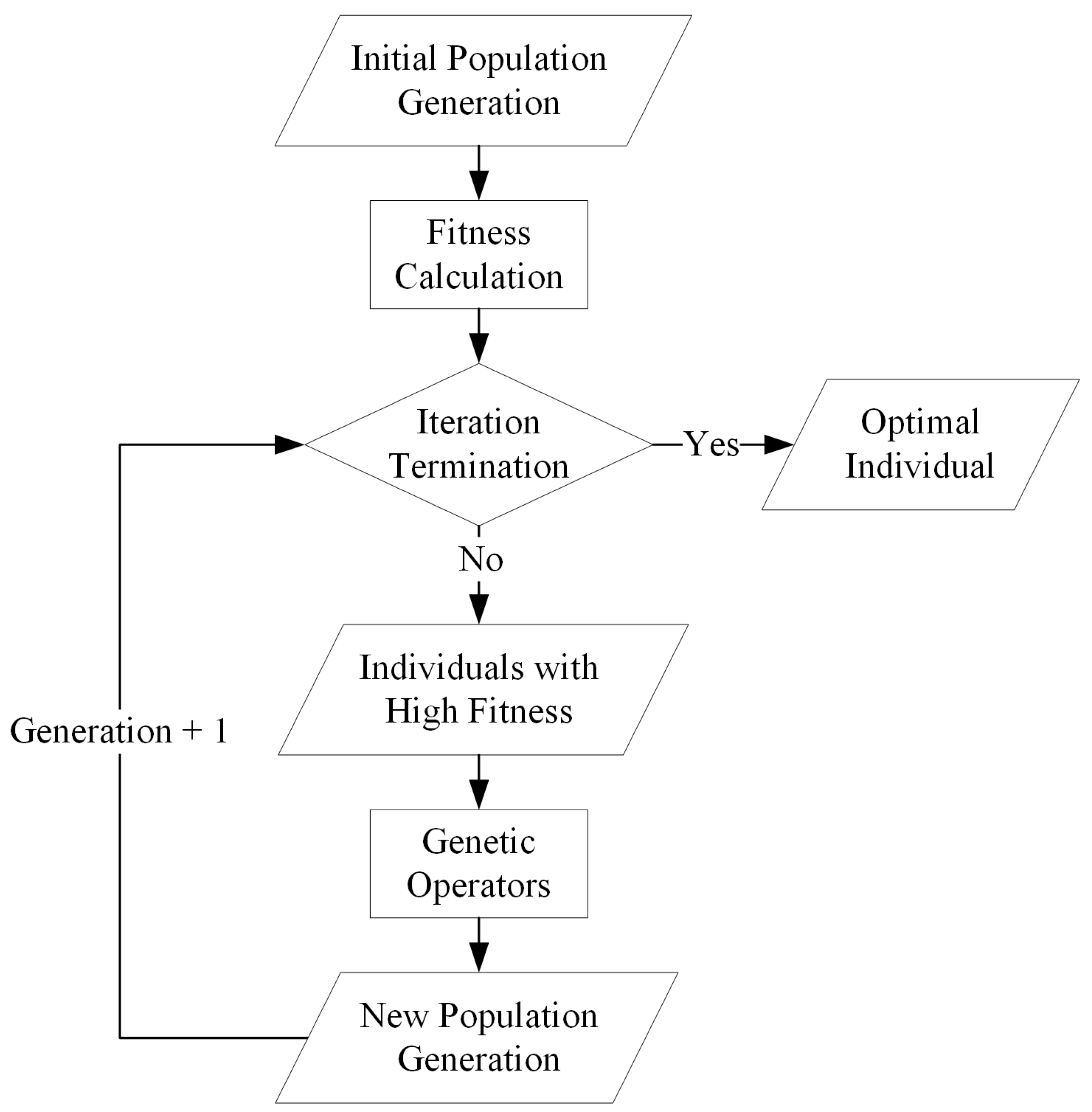
3.3.4. Flow of the GP Algorithm

GP algorithm first constructs several individual trees to form the initial population and then iterates over these trees. After each iteration, the algorithm calculates the fitness of individual trees and determines whether the iteration termination condition is satisfied. The iteration ends if the condition is satisfied. Otherwise, replication, crossover, and mutation operations are performed to generate new individuals to form the next generation of populations for a new iteration. The flowchart of GP algorithm is shown in Figure 8.

In this study, the setting of GP parameters follows a standard GP process [70]. GP first generated 100 individual trees and evaluated their classification accuracy. Then, the top 20% of individuals were selected using the tournament selection method [71], following the criterion of high classification accuracy and few internal nodes. Specifically, first, three individuals were randomly selected from the population, followed by elimination of the individual with the lowest classification accuracy, and then the one with fewer internal nodes was selected from the remaining two individuals and replicated to the next generation population. This procedure was repeated until the number of selected individuals reached 20% of the total population. To creat the rest of individuals of the new population, each selected individuals was replicated five times and subjected to the genetic operation with a 5% crossover rate and a 90% mutation rate to generate new offspring for the next iteration. After each iteration, the individual with the highest classification accuracy was stored, and the current one would be replaced if a higher accuracy was found in the later iterations. The iteration was terminated when 100 iterations were completed (i.e., the generation reached 100), and the individual with the highest classification accuracy recorded in the iteration was selected as the optimal classification model [72].

3.4. Segmentation and Classification Evaluation

The Overall Goodness F-measure (OGF) method was used to measure the segmentation performance in this study. The value of OGF ranged from 0 to 1. The segmentation scale corresponding to the maximum OGF value was used as the optimal scale [73]. OGF was calculated as follows:

$$OGF=\left(1+{\alpha }^2\right)\frac{M{I}_{norm}\times L{V}_{norm}}{{\alpha }^2\times M{I}_{norm}+L{V}_{norm}},$$

(1)

where $M{I}_{norm}$ and $L{V}_{norm}$ represent normalized [0,1] measures of Moran’s I (MI) [74] and local variance (LV) [75]. $\alpha$ is a parameter used to adjust the relative weights of $M{I}_{norm}$ and $L{V}_{norm}$ in Equation (1). $\alpha =1$, $>$1, and $<$1 indicate equal weights for $M{I}_{norm}$ and $L{V}_{norm}$, higher weights for $L{V}_{norm}$, and higher weights for $M{I}_{norm}$, respectively. Usually, the optimal segmentation scale is obtained when these two indicators are balanced, therefore, $\alpha$ was set to 1 in this study [55].

LV was calculated as follows:

$$LV=\frac{1}{n_w\times n_h}\sum _{i=1}^N{a}_i{\sigma }_i,$$

(2)

where $n_w$ and $n_h$ represent the width and height of the image, N is the number of segments, $a_i$ and ${\sigma }_i$ represent the area and standard spectral deviation of the ith segment. A lower LV value indicates a better intra-segment homogeneity [76].

MI was calculated as shown below:

$$MI=\frac{N\times \left({\sum }_{i=1}^N{\sum }_{j=1}^{N,i\ne j}{\omega }_{i,j}\left(x_i-\overline{x}\right)\left(x_j-\overline{x}\right)\right)}{\left({\sum }_{i=1}^N{\sum }_{j=1}^N{\omega }_{i,j}\right)\times \left({\sum }_{i=1}^N{\left(x_i-\overline{x}\right)}^2\right)},$$

(3)

where N represents the number of segments, $x_i$ is the mean value of spectral reflectance of ith segment, and $\overline{x}$ is the mean value of spectral reflectance of the whole image. $w_{i,j}$ is used to measure the spatial adjacency of segment i and j. If segment i and j are adjacent, $w_{i,j}$ = 1, otherwise 0. A lower MI value means a higher inter-segment heterogeneity [77].

The current study determined the classification accuracy using user’s accuracy (UA), producer’s accuracy (PA), overall accuracy (OA), and Kappa coefficient (Kappa). PA and UA were derived from the confusion matrix and were used for determination of the classification effect of each class, whereas OA and kappa were used to evaluate the overall classification results.

4. Results

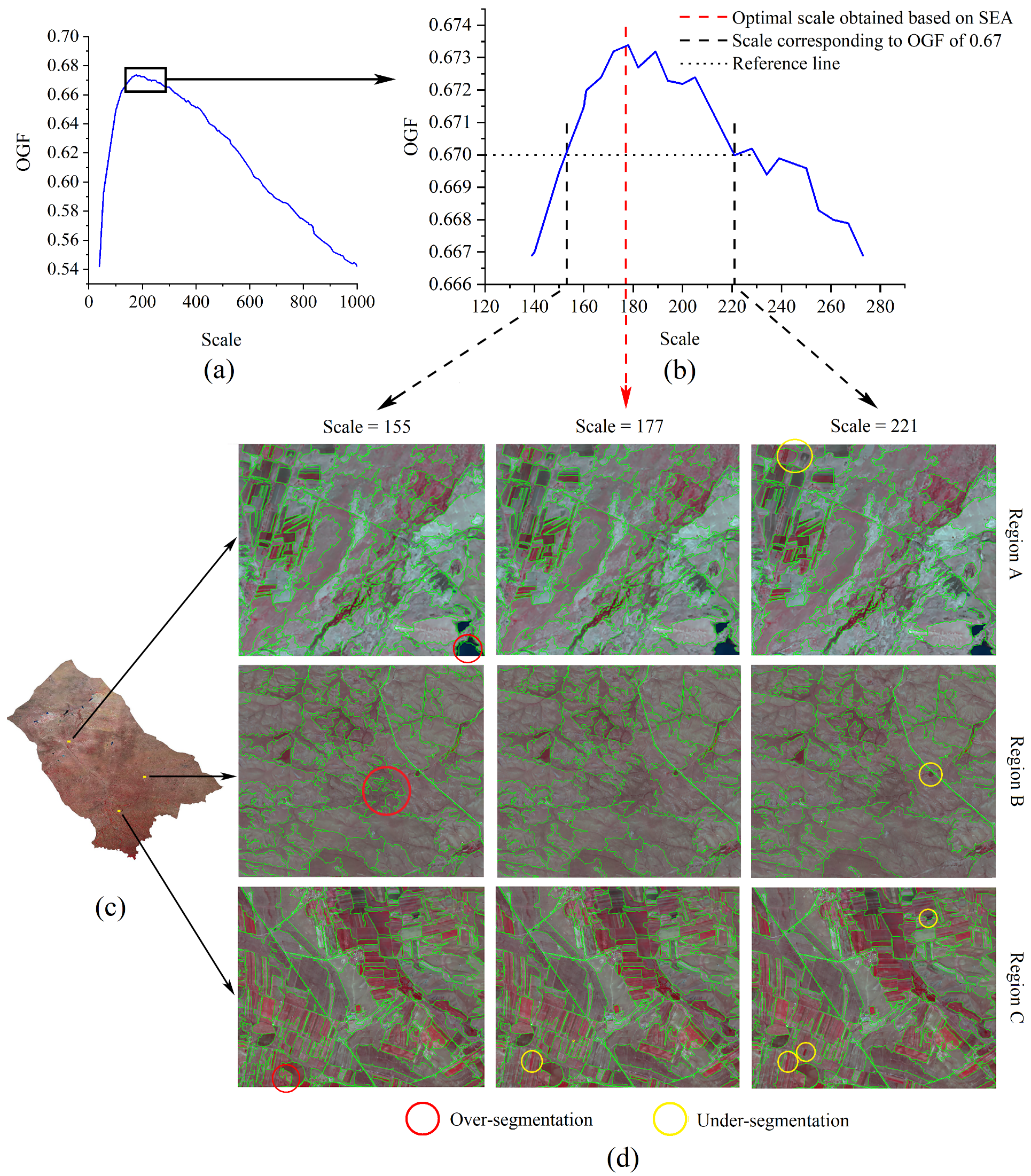
4.1. Segmentation Performance Evaluation

In this study, we performed superpixel segmentation on Sentinel-2 multispectral images based on SEA. To test the segmentation effect of the images under the SEA work, we calculated the OGF values corresponding to the segmentation scales from 0 to 1000. As shown in Figure 9a,b, the OGF curve initially increased and then gradually decreased, and the maximum value was achieved when the scale was close to 180. The optimal scale obtained by the SEA method was 177, and its corresponding OGF value was very close to the peak of the OGF curve. To visually examine the performance of segmentation based on SEA, we compared the segmentation results of three sub-regions within the study area (Figure 8c) at scales larger and smaller than 177 with the OGF value of 0.67 (i.e., 155 and 221) with that of scale 177. As shown in Figure 8d, at 155 scale, there are several fragmented spots in the image due to over-segmentation (yellow markers); at scale 221, there are obvious unsegmented objects (red markers); and at 177 scale, the image visually maintains a relative balance between intra-segmentation homogeneity and inter-segmentation heterogeneity, with few over- and under-segmentation. The results indicated the effectiveness of applying SEA method to achieve accurate segmentation of the images in this study.

4.2. Feature Selection Result

By using RF_RFE, 67 out of 168 features (hereafter MSVT) in Section 3.2 were retained (

Table 5. Feature subset of multispectral and SAR bands, VIs, and textural features screened by RF_RFE.

Categories	Statistics	Features
Spectral Information	Mean	Band 2, 3, 4, 5, 6, 7, 8, 8b
	Standard Deviation	Band 4, 7, 8b
Vegetation Indices	Mean	NDVI, SR, $NDV{I}_{705}$
	Standard Deviation	NDVI, SR, $NDV{I}_{705}$
Textural Features	Mean	Band 2 (Homogeneity, Second Moment, Dissimilarity, Entropy, Correlation) *, Band 4 (Entropy, Homogeneity, Second Moment), Band 7 (Entropy), Band 8 (Second Moment) ${\sigma }_{VV}$ (Second Moment, Entropy, Dissimilarity, Correlation, Contrast, Homogeneity, Variance), ${\sigma }_{VH}$ (Correlation, Second Moment, Entropy, Contrast, Variance, Homogeneity, Dissimilarity)
	Standard Deviation	Band 2 (Homogeneity, Entropy, Correlation) Band 3 (Homogeneity, Entropy), Band 7 (Entropy, Second Moment) Band 4 (Homogeneity, Dissimilarity, Entropy, Correlation), Band 8 (Entropy, Correlation), Band 8b (Entropy, Second Moment) ${\sigma }_{VV}$ (Variance, Contrast, Entropy, Contrast, Second Moment) ${\sigma }_{VH}$ (Second Moment, Correlation)
Backscatter Information	Mean	${\sigma }_{VV}$, ${\sigma }_{VH}$
	Standard Deviation	${\sigma }_{VV}$, ${\sigma }_{VH}$

* denotes the Homogeneity, Dissimilarity, Second Moment, and Entropy of Band 2.

). The more features derived by mean (hereafter MF) were retained compared with those obtained through standard deviation (hereafter SDF), giving a total of 37 and 30 features, respectively. Specifically, for spectral information, the findings for spectral information showed that all spectral bands of MF were retained, whereas only the red and NIR bands were retained in the SDF. This indicated that the spectral information of the superpixels extracted by the mean value was more effective than the standard deviation in this study. For VIs, NDVI, SR, and $NDV{I}_{705}$ were retained in both MF and SDF for VIs, whereas EVI was excluded. For the textural features, MF extracted from SAR images were more retained than those of multispectral images, while the opposite is true for SDF. And for the backscattering information, both MF and SDF of the VV and VH polarization backscattering coefficient were preserved.

To explore the effects of textural features and VIs on classification accuracy of grassland communities in the subsequent experiments, we performed feature selection for the dataset only containing Sentinel-2 multispectral and Sentinel-1 SAR bands, and the results (hereafter MS) are shown in

Table 6. Feature subset of multispectral and SAR bands screened by RF_RFE.

Categories	Statistics	Features
Spectral Information	Mean	Band 2, 3, 4, 7, 8
	Standard Deviation	Band 2, 4
Backscatter Information	Mean	VV, VH
	Standard Deviation	VV

.

4.3. Classification Result Assessment

The optimal classification model for the MSVT dataset generated by GP is shown in Figure 10. The model comprises a primary classifier Linear Support Vector Machine (LinearSVC) and a secondary classifier Extremely Randomized Tree (ET) and uses the stacking strategy [78] to connect them. During the classification process, LinearSVC was first trained with initial samples, and then its training results were used to train ET together with the initial samples. Finally, the final classification results were output by ET.

To evaluate the effectiveness of this fusion model, we classified grassland communities using LinearSVC and ET separately with the same dataset (the hyperparameters of the classifiers remained unchanged) and compared the results with that of the fusion model (

Table 7. OA and Kappa of the six experiments.

Experiment	Classifier (Input Variable)	OA (%)	Kappa
1	LinearSVC + ET (MSVT)	84.21	0.8086
2	LinearSVC (MSVT)	76.32	0.7126
3	ET (MSVT)	73.68	0.6827
4	SVM (MSVT)	75.44	0.7035
5	SVM (MS)	46.49	0.3594
6	GBDT (MS)	59.65	0.5157

and

Table 8. PA and UA of the six experiments.

Experiment	Classifier (Input Variables)	Accuracy (%)	Category
			RES	STC	STT	ARF	STB	STS	ACS
1	LinearSVC+ET (MSVT)	PA	100	84.61	75	100	44.44	85.71	89.29
		UA	87.5	68.75	80	75	80	88.89	92.59
2	LinearSVC (MSVT)	PA	100	81.82	55	85.71	42.86	80.77	80
		UA	81.25	56.25	73.33	75	60	77.78	88.89
3	ET (MSVT)	PA	80	100	63.16	83.33	27.27	80	78.57
		UA	75	62.5	80	62.5	60	74.07	81.48
4	SVM (MSVT)	PA	100	100	57.14	60	44.44	81.48	82.14
		UA	75	43.75	80	75	80	81.48	85.19
5	SVM (MS)	PA	57.89	0	35.71	0	0	62.5	36.36
		UA	78.57	0	47.62	0	0	83.33	80
6	GBDT (MS)	PA	63.64	68.75	46.67	100	44.44	75	45.16
		UA	50	73.33	50	40	30.77	77.78	66.67

). The results of Experiment 1, 2, and 3 showed that the classification accuracies of LinearSVC and ET were similar (76.32% to 74.68%), but both were lower than the accuracy of the fusion model (84.21%).

Three contrast experiments were conducted to validate whether the usage of textural features, VIs, and GP-optimized classification models were able to improve the classification accuracy of grassland community (

Table 9. Optimization results obtained in experiments 4, 5 and 6.

Experiment	Optimization Method	Input Variables	Classifier	Hyperparameter
4	random search	MSVT	SVM	the penalty factor: 16 kernel function: polynomial the parameter coef0 of polynomial: 0.1 the parameter degree of polynomial: 5 the parameter gamma of polynomial: 0.1
5	random search	MS	SVM	radial basis function (RBF) the parameter gamma of RBF: 0.1 kernel function: the penalty factor: 17
6	GP	MS	GBDT	learning rate: 0.1 the number of trees: 100 the maximum depth of a tree: 8 the number of features for splitting: 5 the minimum number of samples in a leaf node: 7 the minimum number of samples for node splitting: 8 the ratio of samples used for training to total samples: 85%

). In Experiment 6, the optimal classification model obtained by GP was the Gradient Boosting Decision Tree (GBDT). The findings showed that the fusion model had the highest classification accuracy for experiments using the MSVT dataset, and there was no significant difference between the results obtained from the three single classifier-based experiments. The classification accuracy of SVM commonly used in the classification of grassland communities was between that obtained using ET and LinearSVC. And experiments using the MS dataset showed that the classification accuracy of the model obtained by GP (i.e., GBDT) was higher than that of SVM by about 13%. In addition, the accuracy of the classification results using the MSVT dataset was significantly higher than those using MS under the same conditions. The classification accuracy of experiment 1 was 24.56% higher compared with that of experiment 6, and the classification accuracy of experiment 4 was 28.95% higher compared with that of experiment 5.

The results from Experiment 1 were used for mapping the Siziwang grassland community. As shown in Figure 11, the seven grassland communities were regionally distributed. The Reaumuria soongarica (Pall.) Maxim grassland and the Stipa caucasica subsp. glareosa (P. A. Smirn.) Tzvelev grassland were mainly concentrated in the north region of Siziwang, the Stipa sareptana var. krylovii (Roshev.) P. C. Kuo & Y. H grassland and the Stipa breviflora Griseb grassland were distributed in the southeast region, the Achnatherum splendens (Trin.) Nevski grassland and the Stipa tianschanica var. gobica (Roshev.) P. C. Kuo & Y. H grassland were mainly grown in the central region, and the Artemisia frigida willd grassland was slightly distributed in the southwest region.

5. Discussion

5.1. The Effect of Input Variables on Classification Accuracy

In this study, we used Sentinel-2 multispectral and Sentinel-1 SAR imagery with large swath width to accommodate regional-scale studies. However, due to the spectral and spatial resolutions of satellite-based RS data are generally low, the phenomenon of “the same object with different spectrum” and “the different object with same spectrum” often occurs when observing grassland communities on a large scale [22,38], thus reducing the accuracy of classification.

To enhance accuracy of classification, textures and VIs were incorporated with regular multispectral and SAR bands for classification. According to the results, the classification accuracy was significantly improved by adding textures and VIs compared to using only regular multispectral and SAR bands, either using the random search or GP-optimized classification model. Taking the SVM-based classification results as an example, the SVM classifier using the MS dataset even after optimization showed limited ability to discriminate among the seven grassland communities in the study area (OA 46%) and showed no ability at all to discriminate against the three communities of STC, STB, and ARF. On the contrary, the SVM using the MSVT dataset showed significant discrimination ability of the three communities, and the OA increased by about 29%.

The above results emphasize the role of textures and VIs extracted from spaceborne RS data in the classification of grassland communities. Yet, current studies suggest that there is still potential for multispectral and SAR imagery to improve the classification accuracy of grassland communities in addition to deriving textures and VIs. On the one hand, given the possible differences in the growth rhythms of different grassland communities [79], the involvement of phenological differences in the growth process of different communities derived from the time-series multispectral data may improve the classification accuracy [80]. On the other hand, the dual-polarization approach of Sentinel-1 limits the extraction of polarization features [41]. If expensive full-polarization SAR images, such as RADARSAT-2 and GaoFen-3, are available in the study, rich polarization features of grasses can be extracted by polarization decomposition methods (e.g., Cloude, Krogager), which can provide more references for classification [15,81].

5.2. The Effect of Classification Model on Classification Accuracy

In addition to using more features, it is essential to optimize the classification model based on the extracted feature set, thus improving the classification accuracy of grassland communities [82]. Therefore, in the current study, the Genetic Programming algorithm was used on the derived feature set to obtain the optimal classification model for that feature set. And our results indicated that both using the MS and MSVT datasets, the classification models optimized using GP yielded more accurate results than SVM, which is commonly used in grassland classification studies [63]. In particular, when using MSVT, GP generated a fusion model consisting of LinearSVC and ET by its easily scalable tree structure [68], with significantly improved classification results compared to single classifiers.

These findings indicate that the classification accuracy of grassland communities can be significantly enhanced by GP-optimized classification models when using the same dataset. Moreover, GP can combine different classifiers using the structural characteristics of individual trees to form complex classification models compared with algorithms such as randomized search and grid search, which can only optimize individual classifiers [67]. And when faced with difficult problems, these fusion models that can achieve complementary advantages among classifiers are reported to perform better compared with single classifiers when solving difficult problems [29].

The above classification models are all based on machine learning algorithms. Currently, deep learning algorithms (DL), represented by convolutional neural networks (CNN), Sparse Coding, and Deep Belief Network (DBN), are gradually being used in RS vegetation classification owing to their ability of deep feature mining [83]. DL with deep network structures allows end-to-end learning thus it can extract deep characteristics of vegetation from RS images without human intervention [84]. We intend to explore the GP-optimized DL model for grassland community classification and expect to improve the classification accuracy further.

5.3. The Universality of the Proposed Method

Universality is an important consideration in evaluating the usefulness of vegetation classification methods. A classification method with high universality means that the method obtained in the current study area can be applied to other areas and still achieve promising results. Therefore, it has a higher application value than the methods with low universality [85,86]. Three key parts of the method that significantly affect the final classification results include segmenting the image at the optimal scale, selecting the optimal subset of features, and generating the optimal classification model. The optimal solutions of the three parts were all determined automatically using the optimization algorithms, thus reducing manual intervention and improves universality of this approach. When this approach is adopted in other study areas, we suppose that it could still perform well owing to its ability to automatically determine the optimal solutions based on new images in each step.

5.4. The Future Work

Benefiting from the large swath width and free of charge of the spaceborne mid-resolution RS images, this research achieved regional scale grassland community classification at low cost. In future studies, we intend to use the proposed method to classify grassland communities at national scales and larger scales, considering that there are few classification products on grassland communities at these scales [15]. However, researching such a large scale requiring a large number of RS images, so we plan to do this work on a cloud platform (e.g., Google Earth Engine [87]) to improve efficiency. With the superior capabilities of the cloud server, we can quickly preprocess and analyze the imagery, which greatly reduces the cost of the work. Meanwhile, we intend to explore DL techniques to build classification models and optimize the structure of classification models using GP algorithms in anticipation of better classification results.

6. Conclusions

In the past, expensive hyperspectral and high-resolution RS images were the major data sources for grassland classification at community level. However, these images are only suitable for small-scale studies due to their small swath width and high prices. For large-scale studies, spaceborne mid-resolution RS images with swath widths of several hundred kilometers are more practical. However, due to the limitation of data quality, it is difficult to distinguish different types of grassland communities using only raw images. To enhance the accuracy of classification using these images, in this study, we proposed a regional-scale superpixel-based grassland communities classification approach using the GP-optimized classification model with Sentinel-2 multispectral bands, their derived VIs and textures, and Sentinel-1 SAR bands and their derived textures. The method was tested in Siziwang grassland of China and achieved an accurate classification of the seven communities with an overall accuracy of 84.21% and a kappa coefficient of 0.81. Our results showed that the addition of VIs and textures, as well as the use of GP-optimized classification models, contribute significantly to the classification accuracy of grassland communities. In addition, the proposed method obtains the optimal segmentation scale, the optimal feature subset, and the optimal classification model by using optimization algorithms instead of manual experiments, which makes it more universal, and thus has a higher application value. This research implies the potential of using VIs and textures extracted from multispectral and SAR imagery, and GP-optimized classification models to improve the classification of grassland communities, also provides a reference for the classification of other vegetation communities over large areas using spaceborne mid-resolution RS images.

References

1. Liu, Q.; Liu, Q.; Meng, X.; Zhang, J.; Yao, F.; Zhang, H. The Impact of Seasonality and Response Period on Qualifying the Relationship between Ecosystem Productivity and Climatic Factors over the Eurasian Steppe. Remote Sens. 2021, 13, 3159. [Google Scholar] [CrossRef]
2. De Simone, W.; Allegrezza, M.; Frattaroli, A.R.; Montecchiari, S.; Tesei, G.; Zuccarello, V.; Di Musciano, M. From Remote Sensing to Species Distribution Modelling: An Integrated Workflow to Monitor Spreading Species in Key Grassland Habitats. Remote Sens. 2021, 13, 1904. [Google Scholar] [CrossRef]
3. Rapinel, S.; Mony, C.; Lecoq, L.; Clement, B.; Thomas, A.; Hubert-Moy, L. Evaluation of Sentinel-2 time-series for mapping floodplain grassland plant communities. Remote Sens. Environ. 2019, 223, 115–129. [Google Scholar] [CrossRef]
4. Adamo, M.; Tomaselli, V.; Tarantino, C.; Vicario, S.; Veronico, G.; Lucas, R.; Blonda, P. Knowledge-based classification of grassland ecosystem based on multi-temporal WorldView-2 data and FAO-LCCS taxonomy. Remote Sens. 2020, 12, 1447. [Google Scholar] [CrossRef]
5. Erinjery, J.J.; Singh, M.; Kent, R. Mapping and assessment of vegetation types in the tropical rainforests of the Western Ghats using multispectral Sentinel-2 and SAR Sentinel-1 satellite imagery. Remote Sens. Environ. 2018, 216, 345–354. [Google Scholar] [CrossRef]
6. Pitkänen, T.P.; Käyhkö, N. Reducing classification error of grassland overgrowth by combing low-density lidar acquisitions and optical remote sensing data. ISPRS J. Photogramm. Remote Sens. 2017, 130, 150–161. [Google Scholar] [CrossRef]
7. Xu, D. Distribution Change and Analysis of Different Grassland Types in Hulunber Grassland. Ph.D. Thesis, Chinese Academy of Agricultural Sciences Dissertation, Beijing, China, 2019. [Google Scholar]
8. Oddi, L.; Cremonese, E.; Ascari, L.; Filippa, G.; Galvagno, M.; Serafino, D.; Cella, U.M.D. Using UAV Imagery to Detect and Map Woody Species Encroachment in a Subalpine Grassland: Advantages and Limits. Remote Sens. 2021, 13, 1239. [Google Scholar] [CrossRef]
9. Dong, X.; Zhang, Z.; Yu, R.; Tian, Q.; Zhu, X. Extraction of information about individual trees from high-spatial-resolution UAV-acquired images of an orchard. Remote Sens. 2020, 12, 133. [Google Scholar] [CrossRef] [Green Version]
10. Melville, B.; Lucieer, A.; Aryal, J. Assessing the impact of spectral resolution on classification of lowland native grassland communities based on field spectroscopy in Tasmania, Australia. Remote Sens. 2018, 10, 308. [Google Scholar] [CrossRef] [Green Version]
11. Melville, B.; Lucieer, A.; Aryal, J. Classification of lowland native grassland communities using hyperspectral Unmanned Aircraft System (UAS) Imagery in the Tasmanian midlands. Drones 2019, 3, 5. [Google Scholar] [CrossRef] [Green Version]
12. Demarchi, L.; Kania, A.; Ciężkowski, W.; Piórkowski, H.; Oświecimska-Piasko, Z.; Chormański, J. Recursive feature elimination and random forest classification of natura 2000 grasslands in lowland river valleys of poland based on airborne hyperspectral and LiDAR data fusion. Remote Sens. 2020, 12, 1842. [Google Scholar] [CrossRef]
13. Zhang, H.K.; Roy, D.P. Using the 500 m MODIS land cover product to derive a consistent continental scale 30 m Landsat land cover classification. Remote Sens. Environ. 2017, 197, 15–34. [Google Scholar] [CrossRef]
14. Yang, L.; Jin, S.; Danielson, P.; Homer, C.; Gass, L.; Bender, S.M.; Case, A.; Costello, C.; Dewitz, J.; Fry, J.; et al. A new generation of the United States National Land Cover Database: Requirements, research priorities, design, and implementation strategies. ISPRS J. Photogramm. Remote Sens. 2018, 146, 108–123. [Google Scholar] [CrossRef]
15. Lopatin, J.; Fassnacht, F.E.; Kattenborn, T.; Schmidtlein, S. Mapping plant species in mixed grassland communities using close range imaging spectroscopy. Remote Sens. Environ. 2017, 201, 12–23. [Google Scholar] [CrossRef]
16. Hong, G.; Zhang, A.; Zhou, F.; Brisco, B. Integration of optical and synthetic aperture radar (SAR) images to differentiate grassland and alfalfa in Prairie area. Int. J. Appl. Earth Obs. Geoinf. 2014, 28, 12–19. [Google Scholar] [CrossRef]
17. Wang, X.; Zhang, S.; Feng, L.; Zhang, J.; Deng, F. Mapping Maize Cultivated Area Combining MODIS EVI Time Series and the Spatial Variations of Phenology over Huanghuaihai Plain. Appl. Sci. 2020, 10, 2667. [Google Scholar] [CrossRef]
18. Wang, C.; Xiao, Z.; Wu, J. Functional connectivity-based classification of autism and control using SVM-RFECV on rs-fMRI data. Phys. Med. 2019, 65, 99–105. [Google Scholar] [CrossRef] [PubMed]
19. Yang, X.; Yang, T.; Ji, Q.; He, Y.; Ghebrezgabher, M.G. Regional-scale grassland classification using moderate-resolution imaging spectrometer datasets based on multistep unsupervised classification and indices suitability analysis. J. Appl. Remote Sens. 2014, 8, 083548. [Google Scholar] [CrossRef]
20. Masjedi, A.; Zoej, M.J.V.; Maghsoudi, Y. Classification of polarimetric SAR images based on modeling contextual information and using texture features. IEEE Trans. Geosci. Remote Sens. 2015, 54, 932–943. [Google Scholar] [CrossRef]
21. Xun, L.; Zhang, J.; Cao, D.; Yang, S.; Yao, F. A novel cotton mapping index combining Sentinel-1 SAR and Sentinel-2 multispectral imagery. ISPRS J. Photogramm. Remote Sens. 2021, 181, 148–166. [Google Scholar] [CrossRef]
22. Khan, I.; Zhang, X.; Rehman, M.; Ali, R. A literature survey and empirical study of meta-learning for classifier selection. IEEE Access 2020, 8, 10262–10281. [Google Scholar] [CrossRef]
23. Prošek, J.; Šímová, P. UAV for mapping shrubland vegetation: Does fusion of spectral and vertical information derived from a single sensor increase the classification accuracy? Int. J. Appl. Earth Obs. Geoinf. 2019, 75, 151–162. [Google Scholar] [CrossRef]
24. Mora, A.; Santos, T.; Łukasik, S.; Silva, J.; Falcão, A.J.; Fonseca, J.M.; Ribeiro, R.A. Land cover classification from multispectral data using computational intelligence tools: A comparative study. Information 2017, 8, 147. [Google Scholar] [CrossRef] [Green Version]
25. Maxwell, A.E.; Warner, T.A.; Fang, F. Implementation of machine-learning classification in remote sensing: An applied review. Int. J. Remote Sens. 2018, 39, 2784–2817. [Google Scholar] [CrossRef] [Green Version]
26. Eiben, A.E.; Schoenauer, M. Evolutionary computing. Inf. Process. Lett. 2002, 82, 1–6. [Google Scholar] [CrossRef]
27. Mehr, A.D.; Nourani, V. A Pareto-optimal moving average-multigene genetic programming model for rainfall-runoff modelling. Environ. Model. Softw. 2017, 92, 239–251. [Google Scholar] [CrossRef]
28. Fayed, H.A.; Atiya, A.F. Speed up grid-search for parameter selection of support vector machines. Appl. Soft Comput. 2019, 80, 202–210. [Google Scholar] [CrossRef]
29. Le, T.T.; Fu, W.; Moore, J.H. Scaling tree-based automated machine learning to biomedical big data with a feature set selector. Bioinformatics 2020, 36, 250–256. [Google Scholar] [CrossRef] [PubMed] [Green Version]
30. Liu, B.; Hu, H.; Wang, H.; Wang, K.; Liu, X.; Yu, W. Superpixel-based classification with an adaptive number of classes for polarimetric SAR images. IEEE Trans. Geosci. Remote Sens. 2012, 51, 907–924. [Google Scholar] [CrossRef]
31. Zhang, G.; Jia, X.; Hu, J. Superpixel-based graphical model for remote sensing image mapping. IEEE Trans. Geosci. Remote Sens. 2015, 53, 5861–5871. [Google Scholar] [CrossRef]
32. Csillik, O. Fast segmentation and classification of very high resolution remote sensing data using SLIC superpixels. Remote Sens. 2017, 9, 243. [Google Scholar] [CrossRef] [Green Version]
33. Farooq, A.; Jia, X.; Hu, J.; Zhou, J. Multi-resolution weed classification via convolutional neural network and superpixel based local binary pattern using remote sensing images. Remote Sens. 2019, 11, 1692. [Google Scholar] [CrossRef] [Green Version]
34. Gao, Y. Research on Landscape Dynamic and Ecological Pattern Optimization in Desert Steppe-Taking the Siziwang Banner of inner Mongolia as an Example. Ph.D. Thesis, Inner Mongolia Agricultural University, Hohhot, China, 2019. [Google Scholar]
35. Wang, D. Study on Community Characteristics of Plants in Peturning Farmland to Grassland in Farming Pastoral Ecotone-Taking Siziwang Banner as an Example. Master’s Thesis, Inner Mongolia Agricultural University, Hohhot, China, 2019. [Google Scholar]
36. Zhang, X. Scrub, Desert, and Steppe. In Vegetation and Its Geographical Pattern in China: An Illustration of the Vegetation Map of the People’s Republic of China (1 : 1000000); Geological Publishing House: Beijing, China, 2007; pp. 257–385. [Google Scholar]
37. Karra, K.; Kontgis, C.; Statman-Weil, Z.; Mazzariello, J.; Mathis, M.; Brumby, S. Global land use/land cover with Sentinel-2 and deep learning. In Proceedings of the IGARSS 2021—2021 IEEE International Geoscience and Remote Sensing Symposium, Brussels, Belgium, 12–16 July 2021. [Google Scholar]
38. Ienco, D.; Interdonato, R.; Gaetano, R.; Minh, D.H.T. Combining Sentinel-1 and Sentinel-2 Satellite Image Time Series for land cover mapping via a multi-source deep learning architecture. ISPRS J. Photogramm. Remote Sens. 2019, 158, 11–22. [Google Scholar] [CrossRef]
39. Torres, R.; Snoeij, P.; Geudtner, D.; Bibby, D.; Davidson, M.; Attema, E.; Potin, P.; Rommen, B.; Floury, N.; Brown, M.; et al. GMES Sentinel-1 mission. Remote Sens. Environ. 2012, 120, 9–24. [Google Scholar] [CrossRef]
40. Mandal, D.; Kumar, V.; Ratha, D.; Dey, S.; Bhattacharya, A.; Lopez-Sanchez, J.M.; McNairn, H.; Rao, Y.S. Dual polarimetric radar vegetation index for crop growth monitoring using sentinel-1 SAR data. Remote Sens. 2020, 247, 111954. [Google Scholar]
41. Filipponi, F. Sentinel-1 GRD Preprocessing Workflow. Proceedings 2019, 18, 11. [Google Scholar] [CrossRef] [Green Version]
42. Abdi, A.M. Land cover and land use classification performance of machine learning algorithms in a boreal landscape using Sentinel-2 data. GISci. Remote Sens. 2020, 57, 1–20. [Google Scholar] [CrossRef] [Green Version]
43. Cordeiro, M.C.; Martinez, J.M.; Peña-Luque, S. Automatic water detection from multidimensional hierarchical clustering for Sentinel-2 images and a comparison with Level 2A processors. Remote Sens. Environ. 2021, 253, 112209. [Google Scholar] [CrossRef]
44. Gascon, F.; Bouzinac, C.; Thépaut, O.; Jung, M.; Francesconi, B.; Louis, J.; Lonjou, V.; Lafrance, B.; Massera, S.; Gaudel-Vacaresse, A.; et al. Copernicus Sentinel-2A calibration and products validation status. Remote Sens. 2017, 9, 584. [Google Scholar] [CrossRef] [Green Version]
45. Su, Y.; Guo, Q.; Hu, T.; Guan, H.; Jin, S.; An, S.; Chen, X.; Guo, K.; Hao, Z.; Hu, Y.; et al. An updated vegetation map of China (1: 1000000). Sci. Bull. 2020, 65, 1125–1136. [Google Scholar] [CrossRef]
46. Yang, J.; Kang, Z.; Cheng, S.; Yang, Z.; Akwensi, P.H. An individual tree segmentation method based on watershed algorithm and three-dimensional spatial distribution analysis from airborne LiDAR point clouds. IEEE J. Sel. Top. Appl. Earth Obs. Remote Sens. 2020, 13, 1055–1067. [Google Scholar] [CrossRef]
47. Biswas, H.; Zhang, K.; Ross, M.S.; Gann, D. Delineation of Tree Patches in a Mangrove-Marsh Transition Zone by Watershed Segmentation of Aerial Photographs. Remote Sens. 2020, 12, 2086. [Google Scholar] [CrossRef]
48. Vincent, L.; Soille, P. Watersheds in digital spaces: An efficient algorithm based on immersion simulations. IEEE Trans. Pattern Anal. Mach. Intell. 1991, 13, 583–598. [Google Scholar] [CrossRef] [Green Version]
49. Zhang, X.; Sun, Y.; Shang, K.; Zhang, L.; Wang, S. Crop classification based on feature band set construction and object-oriented approach using hyperspectral images. IEEE J. Sel. Top. Appl. Earth Obs. Remote Sens. 2016, 9, 4117–4128. [Google Scholar] [CrossRef]
50. Hu, Z.; Li, Q.; Zhang, Q.; Zou, Q.; Wu, Z. Unsupervised simplification of image hierarchies via evolution analysis in scale-sets framework. IEEE Trans. Image Process. 2017, 26, 2394–2407. [Google Scholar] [CrossRef] [PubMed]
51. Guigues, L.; Cocquerez, J.P.; Le Men, H. Scale-sets image analysis. Int. J. Comput. Vis. 2006, 68, 289–317. [Google Scholar] [CrossRef]
52. Vilaplana, V.; Marques, F.; Salembier, P. Binary partition trees for object detection. IEEE Trans. Image Process. 2008, 17, 2201–2216. [Google Scholar] [CrossRef] [PubMed]
53. Davis, D.R.; Kisiel, C.C.; Duckstein, L. Bayesian decision theory applied to design in hydrology. Water Resour. Res. 1972, 8, 33–41. [Google Scholar] [CrossRef]
54. Chen, M.; Ke, Y.; Bai, J.; Li, P.; Lyu, M.; Gong, Z.; Zhou, D. Monitoring early stage invasion of exotic Spartina alterniflora using deep-learning super-resolution techniques based on multisource high-resolution satellite imagery: A case study in the Yellow River Delta, China. Int. J. Appl. Earth Obs. Geoinf. 2020, 92, 102180. [Google Scholar] [CrossRef]
55. Wu, Z.; He, L.; Hu, Z.; Zhang, Y.; Wu, G. Hierarchical segmentation evaluation of region-based image hierarchy. IEEE J. Sel. Top. Appl. Earth Obs. Remote Sens. 2019, 12, 2718–2727. [Google Scholar] [CrossRef]
56. Hu, Z.; Zhang, Q.; Zou, Q.; Li, Q.; Wu, G. Stepwise evolution analysis of the region-merging segmentation for scale parameterization. IEEE J. Sel. Top. Appl. Earth Obs. Remote Sens. 2018, 11, 2461–2472. [Google Scholar] [CrossRef]
57. Cui, J.; Zhang, X.; Wang, W.; Wang, L. Integration of optical and SAR remote sensing images for crop-type mapping based on a novel object-oriented feature selection method. Int. J. Agric. Biol. Eng. 2020, 13, 178–190. [Google Scholar] [CrossRef]
58. Cai, Y.; Li, X.; Zhang, M.; Lin, H. Mapping wetland using the object-based stacked generalization method based on multi-temporal optical and SAR data. Int. J. Appl. Earth Obs. Geoinf. 2020, 92, 102164. [Google Scholar] [CrossRef]
59. Stromann, O.; Nascetti, A.; Yousif, O.; Ban, Y. Dimensionality reduction and feature selection for object-based land cover classification based on Sentinel-1 and Sentinel-2 time series using Google Earth Engine. Remote Sens. 2020, 12, 76. [Google Scholar] [CrossRef] [Green Version]
60. Tucker, C.J. Red and photographic infrared linear combinations for monitoring vegetation. Remote Sens. Environ. 1979, 8, 127–150. [Google Scholar] [CrossRef] [Green Version]
61. Jiang, Z.; Huete, A.R.; Didan, K.; Miura, T. Development of a two-band enhanced vegetation index without a blue band. Remote Sens. Environ. 2008, 112, 3833–3845. [Google Scholar] [CrossRef]
62. Gitelson, A.A.; Gritz, Y.; Merzlyak, M.N. Relationships between leaf chlorophyll content and spectral reflectance and algorithms for non-destructive chlorophyll assessment in higher plant leaves. J. Plant Physiol. 2003, 160, 271–282. [Google Scholar] [CrossRef] [PubMed]
63. Haralick, R.M.; Shanmugam, K.; Dinstein, I.H. Textural features for image classification. IEEE Trans. Syst. Man Cybern. 1973, 6, 610–621. [Google Scholar] [CrossRef] [Green Version]
64. Li, Q.; Wang, C.; Zhang, B.; Lu, L. Object-based crop classification with Landsat-MODIS enhanced time-series data. Remote Sens. 2015, 7, 16091–16107. [Google Scholar] [CrossRef] [Green Version]
65. Misra, P.; Yadav, A.S. Improving the classification accuracy using recursive feature elimination with cross-validation. Int. J. Emerg. Technol. 2020, 11, 659–665. [Google Scholar]
66. Akhtar, F.; Li, J.; Pei, Y.; Xu, Y.; Rajput, A.; Wang, Q. Optimal features subset selection for large for gestational age classification using gridsearch based recursive feature elimination with cross-validation scheme. In Frontier Computing; Hung, J., Yen, N., Chang, J.W., Eds.; Springer: Singapore, 2020; pp. 63–71. [Google Scholar]
67. Pullanagari, R.R.; Kereszturi, G.; Yule, I. Integrating airborne hyperspectral, topographic, and soil data for estimating pasture quality using recursive feature elimination with random forest regression. Remote Sens. 2018, 10, 1117. [Google Scholar] [CrossRef] [Green Version]
68. Koza, J.R.; Koza, J.R. Ruggedness of Genetic Programming. In Genetic Programming: On the Programming of Computers by Means of Natural Selection; MIT Press: Cambridge, MA, USA, 1992; pp. 569–582. [Google Scholar]
69. Xie, C. Video Anomaly Detection in Crowede Scenes Based on Genetic Programming. Master’s Thesis, Nanjing University, Nanjing, China, 2015. [Google Scholar]
70. Olson, R.S.; Moore, J.H. TPOT: A tree-based pipeline optimization tool for automating machine learning. In Proceedings of the Workshop on Automatic Machine Learning; Frank, H., Lars, K., Joaquin, V., Eds.; PMLR: New York, NY, USA, 2016; pp. 66–74. [Google Scholar]
71. Deb, K.; Pratap, A.; Agarwal, S.; Meyarivan, T.A.M.T. A fast and elitist multiobjective genetic algorithm: NSGA-II. IEEE Trans. Evol. Comput. 2002, 6, 182–197. [Google Scholar] [CrossRef] [Green Version]
72. Olson, R.S.; Urbanowicz, R.J.; Andrews, P.C.; Lavender, N.A.; Moore, J.H. Automating biomedical data science through tree-based pipeline optimization. In European Conference on the Applications of Evolutionary Computation; Springer: Cham, Switzerland, 2016; pp. 123–137. [Google Scholar]
73. Johnson, B.A.; Bragais, M.; Endo, I.; Magcale-Macandog, D.B.; Macandog, P.B.M. Image segmentation parameter optimization considering within-and between-segment heterogeneity at multiple scale levels: Test case for mapping residential areas using landsat imagery. ISPRS J. Photogramm. Remote Sens. 2015, 4, 2292–2305. [Google Scholar] [CrossRef] [Green Version]
74. Shortridge, A. Practical limits of Moran’s autocorrelation index for raster class maps. Comput. Environ. Urban Syst. 2007, 31, 362–371. [Google Scholar] [CrossRef]
75. Espindola, G.M.; Camara, G.; Reis, I.A.; Bins, L.S.; Monteiro, A.M. Parameter selection for region-growing image segmentation algorithms using spatial autocorrelation. Int. J. Remote Sens. 2006, 27, 3035–3040. [Google Scholar] [CrossRef]
76. Wang, Y.; Meng, Q.; Qi, Q.; Yang, J.; Liu, Y. Region merging considering within-and between-segment heterogeneity: An improved hybrid remote-sensing image segmentation method. Remote Sens. 2018, 10, 781. [Google Scholar] [CrossRef] [Green Version]
77. Böck, S.; Immitzer, M.; Atzberger, C. On the objectivity of the objective function—Problems with unsupervised segmentation evaluation based on global score and a possible remedy. Remote Sens. 2017, 9, 769. [Google Scholar] [CrossRef] [Green Version]
78. Taghizadeh-Mehrjardi, R.; Schmidt, K.; Amirian-Chakan, A.; Rentschler, T.; Zeraatpisheh, M.; Sarmadian, F.; Valavi, R.; Davatgar, N.; Behrens, T.; Scholten, T. Improving the spatial prediction of soil organic carbon content in two contrasting climatic regions by stacking machine learning models and rescanning covariate space. Remote Sens 2020, 12, 1095. [Google Scholar] [CrossRef] [Green Version]
79. Wang, C.; Guo, H.; Zhang, L.; Qiu, Y.; Sun, Z.; Liao, J.; Liu, G.; Zhang, Y. Improved alpine grassland mapping in the Tibetan Plateau with MODIS time series: A phenology perspective. Int. J. Digit. Earth 2015, 8, 133–152. [Google Scholar] [CrossRef]
80. Zhang, J.; Feng, L.; Yao, F. Improved maize cultivated area estimation over a large scale combining MODIS–EVI time series data and crop phenological information. ISPRS J. Photogramm. Remote Sens. 2014, 94, 102–113. [Google Scholar] [CrossRef]
81. Zhang, H.; Wang, T.; Liu, M.; Jia, M.; Lin, H.; Chu, L.M.; Devlin, A.T. Potential of combining optical and dual polarimetric SAR data for improving mangrove species discrimination using rotation forest. Remote Sens. 2018, 10, 467. [Google Scholar] [CrossRef] [Green Version]
82. Habibi, M.; Sahebi, M.R.; Maghsoudi, Y.; Ghayourmanesh, S. Classification of polarimetric SAR data based on object-based multiple classifiers for urban land-cover. J. Indian Soc. Remote 2016, 44, 855–863. [Google Scholar] [CrossRef]
83. Xun, L.; Zhang, J.; Cao, D.; Wang, J.; Zhang, S.; Yao, F. Mapping cotton cultivated area combining remote sensing with a fused representation-based classification algorithm. Comput. Electron. Agric. 2021, 181, 105940. [Google Scholar] [CrossRef]
84. Kattenborn, T.; Leitloff, J.; Schiefer, F.; Hinz, S. Review on Convolutional Neural Networks (CNN) in vegetation remote sensing. ISPRS J. Photogramm. Remote Sens. 2021, 173, 24–49. [Google Scholar] [CrossRef]
85. Xu, J.; Zhu, Y.; Zhong, R.; Lin, Z.; Xu, J.; Jiang, H.; Li, H.; Lin, T. DeepCropMapping: A multi-temporal deep learning approach with improved spatial generalizability for dynamic corn and soybean mapping. Remote Sens. Environ. 2020, 247, 111946. [Google Scholar] [CrossRef]
86. Meng, B.; Yang, Z.; Yu, H.; Qin, Y.; Sun, Y.; Zhang, J.; Chen, J.; Wang, Z.; Zhang, W.; Li, M.; et al. Mapping of Kobresia pygmaea Community Based on Umanned Aerial Vehicle Technology and Gaofen Remote Sensing Data in Alpine Meadow Grassland: A Case Study in Eastern of Qinghai–Tibetan Plateau. Remote Sens. 2021, 13, 2483. [Google Scholar] [CrossRef]
87. Gorelick, N.; Hancher, M.; Dixon, M.; Ilyushchenko, S.; Thau, D.; Moore, R. Google Earth Engine: Planetary-scale geospatial analysis for everyone. Remote Sens. Environ. 2017, 202, 18–27. [Google Scholar] [CrossRef]
Figure 1. Land cover of Siziwang and samples distribution [37].
Remotesensing 13 04067 g001
Figure 2. The flow chart of the proposed classification method for grassland communities in this paper.
Remotesensing 13 04067 g002
Figure 3. Schematic diagram showing watershed segmentation.
Remotesensing 13 04067 g003
Figure 4. An example of a scale set model.
Remotesensing 13 04067 g004
Figure 5. An example of individual tree.
Remotesensing 13 04067 g005
Figure 6. The crossover process of individual trees ( X Y ) + 3 and ( 9 + 4 ) + ( X ÷ Y ) .
Remotesensing 13 04067 g006
Figure 7. The mutation process of in the individual tree ( X Y ) + 3 .
Remotesensing 13 04067 g007
Figure 8. The flowchart of GP algorithm.
Remotesensing 13 04067 g008
Figure 9. Evaluation of Segmentation Performance. (a) OGF curve corresponding to the segmentation scale from 0 to 1000. (b) OGF curve corresponding to the segmentation scale from 139 to 272. (c) False-color composite Sentinel-2 image of Siziwang on July 3, 2019. (d) Segmentation results for the three subregions of Siziwang at scales of 155, 177, and 221, respectively.
Remotesensing 13 04067 g009
Figure 10. The optimal classification model of the MSVT dataset obtained by GP algorithm.
Remotesensing 13 04067 g010
Figure 11. The classification results of Siziwang grassland community.
Remotesensing 13 04067 g011