Learning Behavior Trees for Autonomous Agents with Hybrid Constraints Evolution


College of Systems Engineering, National University of Defense Technology, Changsha 410073, Hunan, China
*
Author to whom correspondence should be addressed.
Appl. Sci. 2018, 8(7), 1077; https://doi.org/10.3390/app8071077
Submission received: 7 May 2018
/
Revised: 15 June 2018
/
Accepted: 28 June 2018
/
Published: 3 July 2018
(This article belongs to the Special Issue Multi-Agent Systems)
Abstract
:Featured Application
The proposed approach can learn transparent behavior models represented as Behavior Trees, which could be used to alleviate the heaven endeavor of manual agent programming in game and simulation.
Abstract
In modern training, entertainment and education applications, behavior trees (BTs) have already become a fantastic alternative to finite state machines (FSMs) in modeling and controlling autonomous agents. However, it is expensive and inefficient to create BTs for various task scenarios manually. Thus, the genetic programming (GP) approach has been devised to evolve BTs automatically but only received limited success. The standard GP approaches to evolve BTs fail to scale up and to provide good solutions, while GP approaches with domain-specific constraints can accelerate learning but need significant knowledge engineering effort. In this paper, we propose a modified approach, named evolving BTs with hybrid constraints (EBT-HC), to improve the evolution of BTs for autonomous agents. We first propose a novel idea of dynamic constraint based on frequent sub-trees mining, which can accelerate evolution by protecting preponderant behavior sub-trees from undesired crossover. Then we introduce the existing ‘static’ structural constraint into our dynamic constraint to form the evolving BTs with hybrid constraints. The static structure can constrain expected BT form to reduce the size of the search space, thus the hybrid constraints would lead more efficient learning and find better solutions without the loss of the domain-independence. Preliminary experiments, carried out on the Pac-Man game environment, show that the hybrid EBT-HC outperforms other approaches in facilitating the BT design by achieving better behavior performance within fewer generations. Moreover, the generated behavior models by EBT-HC are human readable and easy to be fine-tuned by domain experts.
1. Introduction
Modern training, entertainment and education applications make extensive use of autonomously controlled virtual agents or physical robots [1]. In these applications, the agents must display complex intelligent behaviors to carry out given tasks. Until recently, those behaviors have always been developed using manually designed scripts, finite state machines (FSMs) or behavior trees (BTs) etc. However, these ways may not only impose intensive work on human designers when facing multiple types of agents, missions or scenarios, but also result in rigid and predictable agent behaviors [2,3]. An alternative way is using machine learning (ML) techniques to generate agent behaviors automatically [1,4,5]. Through providing sample traces or evaluation criterion of experts’ desired behavior, an agent can learn behavior model from expert demonstration or trial-and-error experience respectively. Nevertheless, pure ML approaches, like neuron network (NN) or reinforcement learning (RL), usually generate behavior models as black box systems, which are difficult for domain experts to understand, validate and modify [6,7].
Having the advantages of modularity, reactiveness and scalability compared to FSMs, BTs have become a dominant approach to encode embodied agent behavior in computer games, simulation and robotics [8,9]. A BT can be regarded as a hierarchical goal-oriented reactive planner, which can represent not only a static task plan, but also a complex task policy through conditional checks of various situations. Moreover, due to the hierarchical and modular tree structure, BTs are compatible with genetic programming (GP) to perform sub-tree crossover and mutation, which can yield an optimized BT [6]. Furthermore, the well organized behavior model in BT formalism is accessible and easy to fine-tune for domain experts [10,11].
To balance between automatic generation and model accessibility, recently, several researchers are focusing on learning transparent behavior models as BTs, particularly using genetic programming [11,12,13,14]. GP is an evolutionary optimization approach to search an optimal program for a given problem through learning from experience repeatedly [15,16]. The evolving BT is a series of specific approaches which apply GP for agent behavior modeling in certain tasks. The learned model is represented and acted upon in the form of a BT, which is usually evaluated according to a fitness function defined by domain expert based on mission/task. While those approaches have achieved positive results, there are still some open problems [12,14]. For the standard evolving BTs approach (EBT), the global random crossover and mutation would result in dramatically growing trees with many nonsensical branches, which makes it fail to scale up and to provide good solutions. To efficiently generate a good BT solution, some approaches apply a set of domain-specific constraints to reduce the size of the search space, which may limit the application of evolving BTs approaches [13,17].
In this paper, we propose a modified approach, named evolving BTs with hybrid constraints (EBT-HC), to learn behavior models as BTs for autonomous agents. Firstly, a novel idea of dynamic constraint based on frequent sub-trees mining is presented to accelerate learning. It first identifies frequent sub-trees of the superior individuals with higher fitness, then adjusts node crossover probability to protect such preponderant sub-trees from undesired crossover. However, for the large global random search and increasing risk trapped in unwanted local optima, the evolving BTs with only dynamic constraint (EBT-DC) may find unstable solution. Secondly, we extend our dynamic constraint with the existing ‘static’ structural constraint (EBT-SC) [14] to form the evolving BTs with hybrid constraints. The static constraint can set structural guideline for expected BTs to limit the size of search space, thus the hybrid constraints would lead more efficient learning and find better solutions without the loss of the domain-independence. The experiments, carried out on the Pac-Man game environment, show that in most cases the dynamic constraint is effective to help both EBT-DC and EBT-HC to accelerate evolution and find comparable final solutions than the EBT and EBT-SC. However, the solutions found by EBT-DC become more unstable as the diversity of population decreases. The hybrid EBT-HC can outperform other approaches by yielding more stable solutions with higher fitness in fewer generations. Additionally, the resulting BTs and frequent sub-trees found by EBT-HC are comprehensible and easy to analyze and refine.
The remainder of this paper is organized as follows. Section 2 introduces background and related works of agent behavior modeling and evolving BTs. Section 3 describes the proposed evolving BTs with hybrid constraints approach. Section 4 tests the proposed approach in the Pac-Man AI game. Finally, Section 5 draws conclusions and suggests directions for future research.
2. Background and Related Works
In this section, we recall behavior trees and genetic programming as our necessary research background, and review some related works of agent behavior modeling and evolving behavior trees.
2.1. Behavior Trees
A behavior tree can be regarded as a hierarchical plan representation and decision-making tool to encode autonomous agent behavior. It is an intuitive alternative to FSM with modularity and scalability advantages. Thus, experts can decompose a complex task into simple and reusable low level task modules and build them independently. Nowadays BTs have been adopted dominantly to model the behavior of non-player characters (NPC) (a.k.a. computer generated forces (CGF) in simulation) in game industry, and also applied widespread on robotics [10].
A BT is usually defined as a directed rooted tree , where V is the set of all the tree nodes, E is the set of edges to connect tree nodes, is the root node. For each connected node, we define as the outgoing node and as the incoming node. The has no parents and only one child, and the has no child. A single leaf node represents a . In addition, a node between root and leaves represents a combining of primitive behaviors and other composed behaviors, which corresponds to a . The execution of a BT proceeds as follows. Periodically, the node sends a signal called to its children. This tick is then passed down to leaf nodes according to the propagation rule of each node type. Once a leaf node receives a tick, a corresponding behavior is executed. The node returns to its parent status if its execution has not finished yet, if it has achieved its goal, or otherwise.
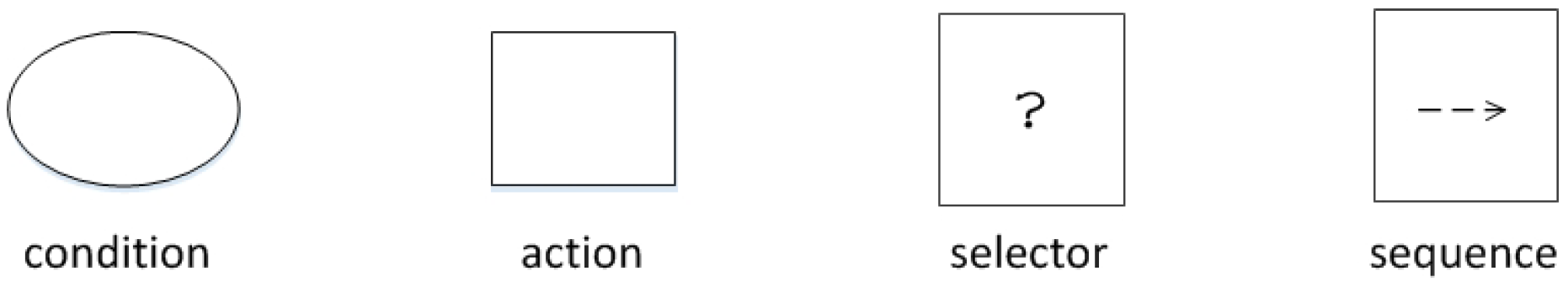
In this paper, we adopt the BTs building approach recommended in [18], whose components include , , and nodes.
: The condition node checks whenever a condition is satisfied or not, returning or accordingly. The condition node never returns .
: a selector node propagates the tick signal to its children sequentially. If any child returns or , the stops the propagation and returns the received state. If all children return , the Selector returns .
: a sequence node also propagates the tick signal to its children sequentially. However, if any child returns or , the stops the propagation and returns the received state. Only if all children return , the Sequence returns .
: The action node performs a primitive behavior, returning if the action is completed and if the action cannot be completed. Otherwise it returns .
Figure 1 shows the graphical representation of all types of nodes used in this paper.
2.2. Genetic Programming
Genetic programming is a specialization of genetic algorithms which performs a stochastic search to solve a particular task inspired by Darwin’s theories of evolution [15,16]. In GP, each individual within the evolving population represents a computer program, which typically is a tree structure such as a behavior tree. The evolving BTs approach applies GP to optimize a population of randomly-generated BTs for agent behavior modeling. Each BT represents a possible behavior model to control autonomous agent evaluated according to a fitness function defined by domain expert based on task. The learning goal is to find a BT controller which can maximize the fitness in the task. For a BT controller, possible states related to decision-making are encoded as condition nodes, available primitive actions in the task are encoded as action nodes, decision-making logic is controlled by BT composite nodes (such as selector, sequence or parallel), a behavior policy is a tree individual with ordered composition of control nodes and leaf nodes.
For BT populations, individuals are evolved using genetic operations of reproduction, crossover, and mutation. In each iteration of the algorithm, some fitter individuals are selected for reproduction directly. Some individuals take crossover operation where a random sub-tree from one individual is swapped with a random sub-tree from another individual and produce two new trees for the next generation. A mutation operator that randomly produces small changes to individuals is also used in order to increase diversity within the population. This process continues until the GP finds a BT that satisfies the goal (e.g., minimize the fitness function and satisfy all constraints).
Often, the crossover operation can bring on undesirable effect of rapidly increasing tree sizes for final generated BT. This phenomenon of generating a BT of larger size than necessary can be termed as bloat. Several approaches for dealing with bloat have been developed [16]. These approaches essentially have a fitness cost based on the size of the tree, thus increasing the tendency for more compact tree to be selected for reproduction.
2.3. Agent Behavior Modeling and Evolving Behavior Trees
In computer games and simulation, a variety of agent programming techniques have been employed to represent and embed agent behaviors, especially for decision-making process. Those techniques usually encode agent behaviors in well-defined structures/models based on domain expertise and customizable constrains, such as FSMs, hierarchical finite state machines (HFSMs), rule-based systems and BTs etc. [2,3]. Among which, BTs have come to the forefront recently for their modularity, scalability, reusability and accessibility [8,9,10]. However, most of the developments based on those scripting approaches rely on domain expertise and suffer from time-consuming, expensive and difficult endeavor of programming complexity [2,4,19].
On the other side of the spectrum, various approaches are emerged in machine learning community to generate adaptive agent behavior automatically [5,20,21,22]. This field has been studied basically from two perspectives [1,2]: learning from observation (LfO) (a.k.a, learning from demonstration, programming from demonstration) and learning from experience. The former allows agent to extract the behavior model of the target agent by observing the behavior trace of another agent (e.g., using NN and case-based learning) [4,20]. For example, Fernlund et al. [20] adopted LfO to build agents capable of driving a simulated automobile in a city environment. Ontañón et al. [23] use learning from demonstration for realtime strategy games in the context of case-based planning. While the later leads virtual agent to learn and optimize its behavior by interacting with environment repeatedly (e.g., reinforcement learning and evolutionary algorithms) [5,22]. The performance of the agent is measured according to how well the task is performed as expert’s evaluation criterions, which may sometimes find creative solutions that are not found by humans termed as computational creativity [4]. For instance, Aihe and Gonzalez [24], propose Reinforcement learning (RL) to compensate for situations where the domain expert has limited knowledge of the subject being modeled. Teng et al. [22] use a self-organizing neural network to learn incrementally through real-time interactions with the environment, which can improve air combat maneuvering strategies of CGFs. Please note that most of those machine learning methods generate behavior model as a black box system [6,7]. As a result, domain expert could not produce a clear explanation of the relationship between behaviors and models, which is hard to analyze and validate.
To remedy the disadvantages, in both behavior learning perspectives, there are some attempts to generate behavior models represented as BTs from observation [7,25] or experience [11,12,14,26,27] automatically. In this paper, we are focusing on generate BTs through experiential learning, especially evolving BTs. Please note that comparing with other policy representation approaches (decision tree etc.), BT is a more flexible representation which allows explicitly a course of actions as a sub-policy for certain situation. Therefore, for evolving BTs, the scalability is still an open problem stemming from the random large space search [12,14]. In [12], the author points out it is too flexible for evolving BTs without structural guidelines, which would result in most trees that are quite inefficient and impossible to read. So the author constrains the crossover with fixed ’behavior block’ sub-trees, which yield comparable reactive behavior. In [14], the authors investigate the effect of ’standard BT design’ constraint on evolving BTs approach, which is domain-independent and efficient. They also point out most existing evolving BT approaches adopt different manual constraints to design what the BTs represent and the nature of the tree’s constraints. Some of those approaches can speed up learning efficiently but need a lot of knowledge engineering works, which may limit the application of evolving BT approaches. For instance, Scheper et al. [17] apply genetic algorithm to generate improved BTs for a real-world robotic, the initial creation of the trees are not random but human design. In [13], the whole task in game DEFCON is decomposed into a series of sub-tasks and the learning task is just to evolve simple parameter for each sub-task respectively.
Even though the works mentioned above cover most aspects of the behavior modeling with evolving BTs, we intend to use a model-free dynamic constraint to accelerate evolution. We base our work on the standard evolving BTs approach. The main concern is around how to apply model-free constraint or heuristic to speed up BT evolving.
3. Methodology
In this section, we give details about our proposed approach in mainly tow folds. Firstly, we show an overview of the proposed framework, including its main components and basic workflow. Secondly, we elaborate the proposed dynamic constraint and how we extend it with the existing static structural constraint.
3.1. The Proposed Evolving Behavior Trees Framework
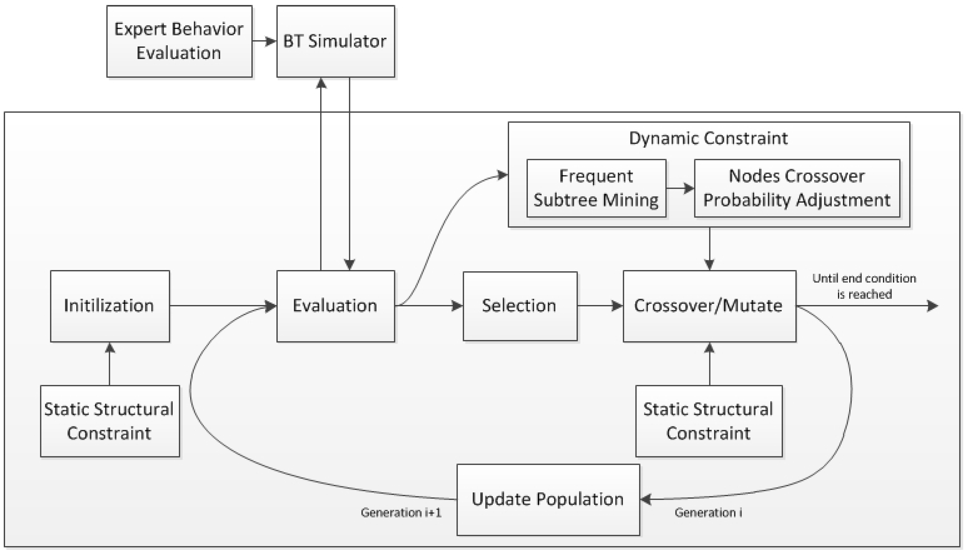
Our proposed approach, evolving BTs with hybrid constraints (EBT-HC), is outlined in Figure 2. As the figure shows, two new components, ‘Static Structural Constraint’ and ‘Dynamic Constraint’, are added and interacted with the standard evolving BTs process. For the static structural constraint, it set some tree rules to constrain expected BT structure in population initialization and crossover, which can avoid many meaningless and inefficient tree configurations in evolution. For the dynamic constraint, it first applies frequent sub-trees mining for a few higher ranked individuals in each generation, then adjusts nodes crossover probabilities based on the extracted frequent sub-trees, which can protect preponderant structures against undesirable crossover.
In detail, the workflow of the proposed EBT-HC for agent behavior modeling can be described as follows:
At first, the GP system creates initial BT population individuals under static structural constraint. Unlike fully random combination of leaf nodes and control nodes in standard evolving BTs, the initial BTs are generated constrained by predefined BT syntax rules which will be elaborated in Section 3.3.
Secondly, the GP system evaluates each individual in the population respectively, which needs to run the BT simulator and calculate fitness according to the simulation results and behavior evaluation function. The BT simulator simulates the task execution with the agent controlled by the evaluated BT individual, the behavior evaluation function depicts desired behavior effect quantitatively, which will serve as the fitness measure base that determines the appropriateness of the individuals being evolved.
Thirdly and foremost, some superior individuals with higher fitness are selected to perform crossover and mutate operations to reproduce offsprings. Here we adopt tournament select, sub-tree crossover and single point mutation. Please note that in the sub-tree crossover, the select of crossover node should be constrained by both static structural constraint and dynamic constraint.
Before crossover, we execute a FREQT similar tree mining algorithm for the population and find frequent sub-trees as preponderant structure needing to protect. For each tree individual, according to whether a node belongs to a frequent sub-tree found, we classify nodes in this tree (except the root node) to two sets, protected nodes and unprotected nodes. Then we adjust selected crossover probability of each node accordingly. In brief, we increase the selected probability of unprotected nodes and reduce the selected probability of protected nodes to avoid undesired crossover.
After genetic operation, we update the population to next generation to continue evolution until the end condition is reached.
3.2. Dynamic Constrain Based on Frequent Sub-Tree Mining
In genetic programming, the learner selects preponderant individuals of the current population to reproduce offspring through select operator (e.g., tournament, wheel roulette). From another perspective, the evolution to find an optimal BT is also the process of preponderant structures combination, where a preponderant structure is usually a self-contained behavior sub-tree to deal with certain local situation correctly. So regarding the population individuals as dataset, in each generation, we can mine frequent sub-tree structures of higher fitness individuals. After that we adjust nodes crossover probability to protect such sub-trees against destroyed for faster experiential learning. We call such soft way as dynamic constraint based on frequent sub-tree mining. The intuition behind dynamic constraint is that a frequent sub-tree in superior individuals has a bigger chance to be required by most individuals with higher fitness, even as a sub-tree of the optimal target BT. Thus, we should give more chance to protect such preponderant sub-trees for inherited to next generation. Through preference of crossover nodes based on frequent sub-trees found, in the next generation, there will be more individuals containing those frequent sub-trees, which would lead more precise search around problem space based on those frequent sub-trees, and increase the chance to find a better solution.
In detail, there are two steps to apply dynamic constraint in evolution, frequent sub-tree mining and nodes crossover probability adjustment.
3.2.1. Frequent Sub-Tree Mining
In this section, an adaptation of FREQT [28] is used to mine frequent sub-tree structures in population. FREQT is a classic pattern mining algorithm to discover frequent tree patterns from a collection of labeled ordered trees (LOT). It adopts technique to construct candidate frequent patterns incrementally. At the same time, frequencies of the candidates are computed by maintaining only the occurrences of the rightmost leaf efficiently. It has been demonstrated that FREQT can scale almost linearly in the total size of maximal tree patterns slightly depending on the size of the longest pattern [28,29].
A labeled ordered tree usually represents a semi-structured data structure such as XML. According to the structure and semantics, a behavior tree is a typical labeled ordered tree. Thus the formalism of BT can be expanded from definition of LOT as , where is the basic structure of a BT, is the root node. The mapping is the labeling function, includes the labels of root node, control nodes and leaf nodes (condition nodes and action nodes) of a BT. The binary relation represents a sibling relation for two nodes in a BT. For two nodes and of the same parent, iff then is an elder brother of . The execution of BT is following order of depth first from left to right, ⪯ represents execution orders of two nodes. Thus, we can construct indexes for all the nodes as depth first in an LOT, which can be consistent with records in GP.
Let be the dataset of tree mining, which includes a small fraction of individuals with higher fitness in current population. is a candidate frequent pattern, which is usually a sub-tree in tree mining. is the frequency of in a tree T, depicts whether exists in T. There is if , else . represents the number of trees where frequent pattern sub-tree exists. depicts terminal node size of frequent pattern tree in tree T.
To adapt the notions from FREQT to BTs mining in GP system, we modify the rules to judge whether a sub-tree is frequent. According to BT syntax and its design pattern, a tree can be regarded as a frequent pattern iff it satisfies all the following proposed rules.
- and , where depicts the minimal support of a frequent pattern, depicts the minimal node size of a frequent pattern and depicts the maximal node size of a frequent pattern.
- All terminal nodes in a frequent pattern must be leaf nodes (condition nodes or action nodes).
- , where depicts the minimal terminal node size of a frequent pattern.
Rule 1 is the basic requirement of FREQT data mining algorithms. Rule 2 and rule 3 represent proposed form requirements of expected patterns in behavior modeling with BT. As a decision making tool, the core of a BT is rooted in the logic relation among its leaf nodes. Thus, in rule 2, we believe if a terminal node is a control node, it is meaningless for its located branch. For rule 3, if a frequent pattern has too few terminal nodes (for example only one terminal node), it shows trivial effect on the whole tree construction.
3.2.2. Nodes Crossover Probability Adjustment
After finding the frequent sub-trees collection, the crossover probability of each node is adjusted according to its relation to discovered frequent sub-trees, which can protect those preponderant structures to be inherited to the next generation more likely.
Formally, let depict the set of the selected superior individuals of BTs population at generation i, T is a chromosome tree selected for crossover in , is the set of all the tree nodes in T except the root node . Let depict the set of the mined frequent sub-trees in , is a frequent sub-tree in , is the set of all the tree nodes in , where we define as the root node of , as the set of nodes in .
Provided we find N distinct frequent sub-trees in T, , . Then for the tree T, we define the root node set , the inside node set , and the other node set . To protect the frequent sub-trees unbroken more likely in crossover, we can classify to two sets, protected nodes set and unprotected nodes set . That is, , which stores nodes needing to be protected in T, and , which stores nodes to be unprotected in T.
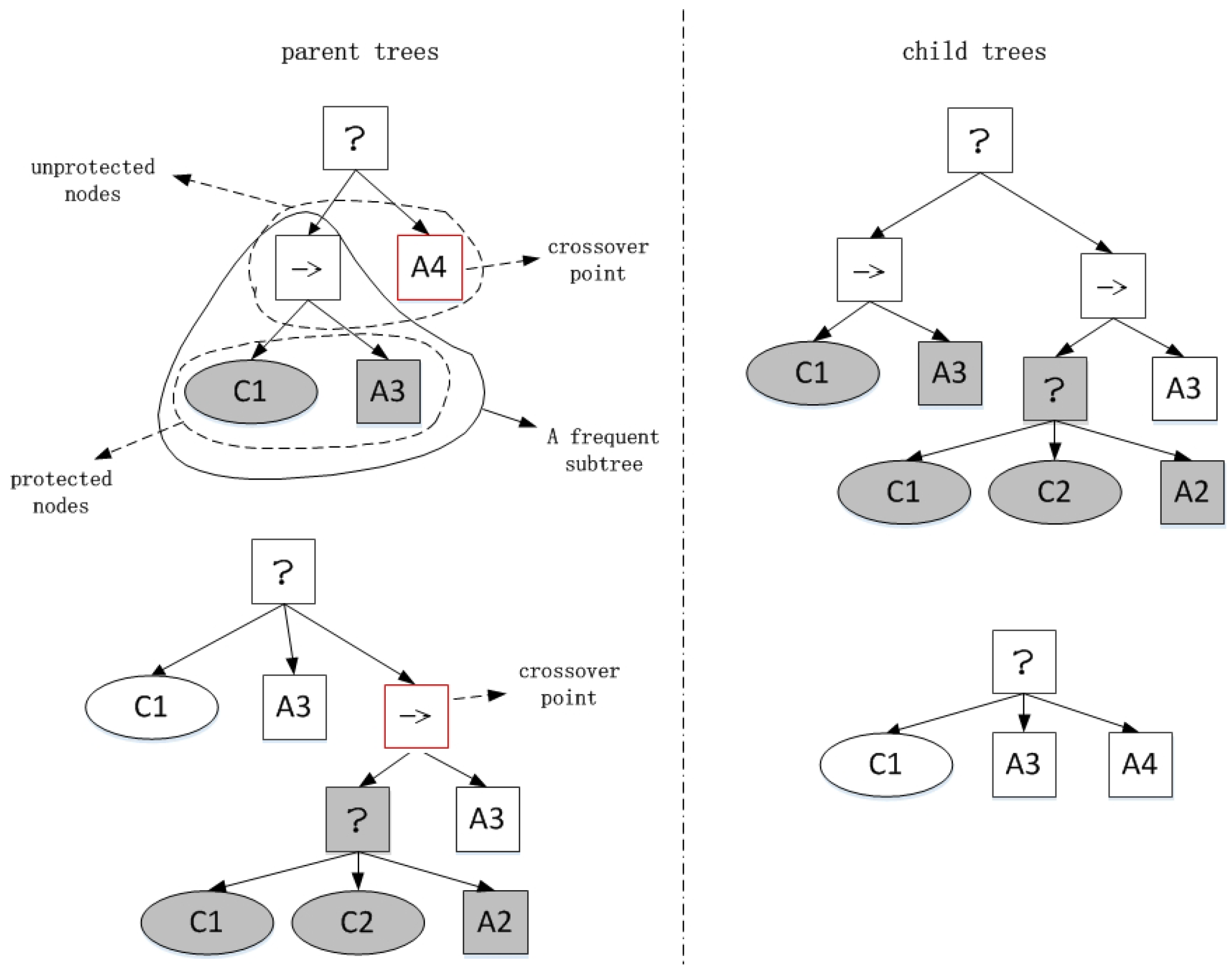
Obviously, to protect preponderant sub-trees inherited to the next generation, we should decrease the select probability of nodes in and increase the select probability of nodes in as crossover point. We consider the fact that standard sub-tree crossover operation produce two child trees, as illustrated in Figure 3.
As we can see in the leftup parent tree, except the root node, its nodes are classified to unprotected nodes and protected nodes enclosed with two dashed curves respectively. The mined frequent sub-tree is enclosed with a non-dashed curve including all the protected nodes and the root node of the frequent sub-tree. Let us denote the select probability as a crossover point at a node v by . The GP system picks up two individuals (e.g., by a tournament selection) from the population, and performs a crossover operation at a node v with the probability , which has been modified and normalized as follows:
where depicts the discount factor, which control the select probability preference for nodes in the protected nodes set.
In Figure 3, the light protected nodes have more chance to be selected in crossover, node ‘A4’ with red square in the figure. Then two sub-trees including preponderant structures will be combined in the right up child tree inherited to next generation. Besides, we can see in Equations (1) and (2), if we cannot find any frequent sub-trees, there is no effect on the standard evolving process. With generation increasing, the crossover probability adjustment would have bigger effect on exploiting frequent preponderant sub-trees.
3.3. Evolving BTs with Hybrid Constraints
Although the idea behind dynamic constraint based on frequent sub-tree mining is intuitive to accelerate evolution, we found it cannot achieve expected performance in some real applications. For standard evolving BT approach, the global random crossover and mutation result in dramatically growing trees with many nonsensical branches. Therefore, it is hard for the standard evolving BT approach to escape from the local minimum, and some frequent patterns found may be inefficient with inactive nodes never to be executed. In this section, we extend our dynamic constraint with the existing static structural constraint [14]. The static constraint sets structural guideline for generated BTs in initiation and crossover, the dynamic constraint adjusts nodes crossover probability to protect preponderant structure based on constrained configuration space, which can lead more efficient learning.
The static structural constraint is referred from paper [14], which enforce following tree rules as ‘standard behavior tree design’:
- Selector node may only be placed at depth levels that are even.
- Sequence node may only be placed at depth levels that are odd.
- All terminal child nodes of a node must be adjacent, and those child nodes must be one or more condition nodes followed by on or more action nodes. If there is only one terminal child node, it must be an action node.
Figure 4 is an example generated BT using above static structural constraint. The generated initial BT individuals are efficient and well understood. To ensure the static structural constraint conformed in evolution, the adjacent terminal child nodes of a node will be regarded as a sequential block to swap together.
To combine dynamic constraint with static structural constraint in evolution, the following two points should be taken into account for Section 3.2:
1. The available selected units are changed in evolving BTs with hybrid constraint.
In evolving BTs based on dynamic constraint, we sort all nodes in a tree to either protected nodes set or unprotected nodes set. While in evolving BTs with hybrid constraints, the candidate nodes to be sorted are subset of all the tree nodes. On one hand, in each parent tree, we regard the adjacent terminal child nodes as a sequential block to crossover as Figure 4. So the size of candidate nodes to be sorted is the sum of control nodes and blocks. Under static constraint, the adjacent terminal child nodes are regarded as a sequential behavior block and the crossover is constrained only between nodes/blocks with the same type, so the possible behavior blocks will be unchanged in crossover, which will reduce the population diversity and limit the search for possible solution. Thus, we should set a high mutation probability to maintain the diversity of generated behavior blocks. On the other hand, for the crossover node in the first parent tree, candidate nodes can be control nodes or blocks, while for the crossover nodes in the second selected parent tree, the crossover node must be the same type as the selected node in the first tree to keep the static structural constraint unbroken, here types include sequence, selector or terminal block.
2. Nodes crossover probability is adjusted based on step 1.
After modifying the candidate nodes in step 1, the crossover probability of nodes should be adjusted accordingly in Section 3.2.2. It should be noted that iff all nodes in a sequential block are in a frequent sub-tree found, the block can be protected.
4. Experimental Section
In this section, a series of experiments are carried out in the Pacman AI open-source benchmark to test the performance of our approach in agent behavior modeling. The experiments are run single threaded on an Intel Core i7, 3.40 GHz CPU using the Windows 7 64-bit operating system. Four evolving BTs approaches with different constraints and a handcrafted BT are compared, the training and final test performance are monitored over time, along with other statistical measurements. The main goal of our experiments is to demonstrate whether our proposed dynamic constraint can help the original approaches to accelerate behavior trees generation and reach comparable behavior performance. Another goal is to ascertain whether we can get useful behavior sub-trees and well-designed final behavior model as handcrafted BTs.
4.1. Simulation Environment and Agents
Our experiments are tested in the ‘Ms. Pac-Man vs Ghosts’ game competition environment [30], which provides available AI API for the original arcade game Ms. Pac-Man. As Figure 5 shows, this game consists of 5 agents, a single Ms. Pac-Man and 4 Ghost agents. In the game, the player, controlling Pac-Man, must navigate a maze-like level to collect pills and avoid enemy ghosts or else lose a life. After collecting large ‘power’ pills, Pac-Man can consume the ghosts and score additional points in a limited period of time. When all the pills in the level are collected the player moves on to the next level, but if three lives are lost the game is over. The only actions available to the player are movement in a 2-dimensional space along the cardinal directions (up, down, left and right), which makes the action space very small. However, the behavior of an AI agent for this game can be quite complex, making it a suitable candidate for the experiments. The scoring method for the game is as follows: eating a normal pill earns Pac-Man 10 points, eating a power pill earns Pac-Man 50 points, and eating ghosts earn 200 points for the first ghost but doubling each time up to 1600 points for the fourth ghost.
To test our evolving BTs approach for agent behavior modeling, we integrate behavior trees and genetic programming into the ‘Ms Pac-Man vs Ghost’ API to model Pac-Man behavior. The ghosts are controlled by the basic script provided in the competition, in which ghosts can communicate to share their perception and choose action with a little randomness. The design of behavior trees for Pan-Man agent are modeled on [18], with the components used including sequence, selector, condition and action nodes. So the function set in GP contains ‘sequence’ and ‘selector’, and the terminal set contains several game-related conditions and actions. At each time step, the game environment requests a single move (up, down, left, right, no move) from the AI agent, which is returned by executing the behavior tree. The actions and conditions are defined as [14], which can be implemented easily by API provided:
- Conditions/////, six condition nodes which return ‘true’ if there is a ghost in the ‘Inedible’ state within a certain fixed distance range, as well as targeting that ghost., ////, six condition nodes which return ‘true’ if there is a ghost in the ‘Edible’ state within a certain fixed distance range, as well as targeting that ghost.//, three condition nodes which return ‘true’ if a previous condition node has targeted a ghost, which is edible and whose remaining time in the ‘edible’ state is within a certain fixed range.//, three condition nodes which return ‘true’ if the current point value for eating a ghost is 400/800/1600.
- Actions: an action node which set Pac-Man’s direction to the nearest pill or power pill, returning ‘true’ if any such pill exists in the level or ‘false’ otherwise.: an action node which set Pac-Man’s direction to the nearest normal pill, returning ‘true’ if any such pill exists in the level or ‘false’ otherwise.: an action node which set Pac-Man’s direction to the nearest power pill, returning ‘true’ if any such pill exists in the level or ‘false’ otherwise.: an action node which set Pac-Man’s direction away from the nearest ghost that was targeted in the last condition node executed, returning ‘true’ if a ghost has been targeted or ‘false’ otherwise.: an action node which set Pac-Man’s direction towards the ghost that was targeted in the last condition node executed, returning ‘true’ if a ghost has been targeted or ‘false’ otherwise.
- Fitness FunctionThe fitness function is the sum of averaged game score and a parsimony pressure value as formula [16]. Where x is the evaluated BT, is the fitness value, is the averaged game score for a few game runs, c is a constant value known as the parsimony coefficient, is the node size of x. The simple parsimony pressure can adjust the original fitness based on the size of BT, which will increase the tendency for more compact tree to be selected for reproduction.
4.2. Experimental Setup
In the experiments, four evolving BTs approaches with different constraints are implemented to make comparison. Those are standard evolving BTs, evolving BTs with static constraint, evolving BTs with dynamic constraint, and evolving BTs with hybrid constraints, which are denoted simply as EBT, EBT-SC, EBT-DC and EBT-HC respectively. A handcrafted BT denoted as Hand is also created manually in order to provide a baseline comparison, which is provided by the competition [30]. The handcrafted BT follows some simple sequential rules: initially checking if any inedible ghosts were too close and moving away from them before moving to chase nearby edible ghosts. If there are no ghosts within range, Pac-Man would travel to the closest pill.
The parameter settings for four evolving BTs approaches are listed as Table 1. Please note that all four approaches use crossover operator to produce two child trees from two parent trees. The main differences are the crossover node select and mutation probability as follows. For the approach EBT, each node, except the root node, has equal chance to be selected as a crossover point. For the approach EBT-SC, the adjacent terminal nodes are regarded as a sequential block, all the control nodes and blocks has equal chance to be selected and swapped. The second crossover node must be the same type as the first selected one. For the approach EBT-DC, each node is selected according to adjusted probability. For the approach EBT-HC, the crossover is similar to the approach EBT-SC, but node select probability is adjusted based on frequent sub-trees found. For the approaches EBT-DC and EBT-HC, the minimal support for frequent sub-trees are set as 0.3, the minimal node size of a frequent sub-tree is set as 3, the minimal terminal node size is set as 2, the maximal terminal node size is set as 15. The discount factor is set as 0.9.
To validate the robustness of the proposed approach, a few GA parameters are selected to be variable for the same game scenario. Specifically, we vary three important GA parameters (crossover probability, new chromosomes, and mutation probability) and report 9 results of different combinations for the four evolving approaches. Please note that the sum of crossover probability and reproduction probability is always equal to 1. The number of full variable parameters combination can be very big, thus we adopt following combination strategy. First we set a group of common GA parameters as basis, with crossover proportion 0.9, new chromosomes 0.3, and mutation probability 0.01. Because under static constraint, the adjacent terminal child nodes are regarded as a sequential behavior block and the crossover is constrained only between nodes/blocks with the same type, so the population diversity is reduced greatly. Thus, we set a high mutation probability of 0.1 as basic value for the EBT-SC and EBT-HC to increase the diversity of generated behavior blocks. For example, when new chromosomes and mutation probability are fixed as 0.3 and 0.01/0.1 (EBT, EBT-DC/EBT-SC, EBT-HC correspondingly), the crossover probability is set as different values of 0.6, 0.7, 0.8 and 0.9 respectively. Similarly, the new chromosomes is set as different values of 0.1, 0.2 and 0.3 respectively, and the mutation probability is set as different values of 0.01 and 0.1 respectively. So we get 9(4 + 3 + 2) experimental results for all the evolving approaches.
For each evolving approach, agents are trained for 100 generations with corresponding configuration and the resulting BT with highest averaged fitness is then played 1000 game runs. Please note that in each generation, each individual is evaluated for 100 game runs to get an expected score as fitness, which is used to reduce the effect of game randomness. All above evolving processes are averaged across 10 trials.
4.3. Results and Analysis
During the learning process, we record all fitness values of individuals and frequent sub-trees found for each generation. After finishing learning, the final test results for generated best individual, the frequent sub-trees found and the final generated BTs are also recorded as results to evaluate the generated behavior models.
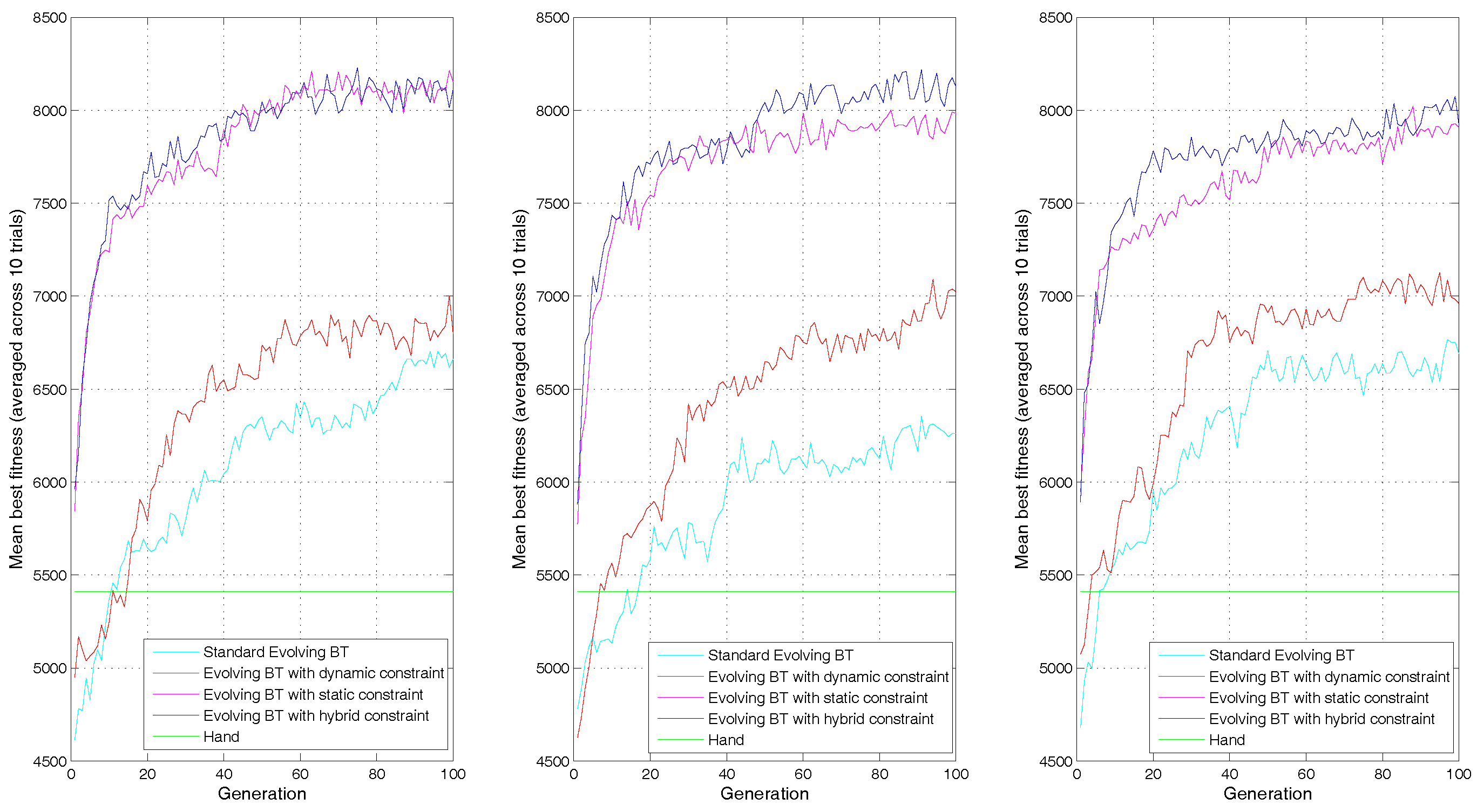
Figure 6, Figure 7 and Figure 8 show the learning curves of mean best fitness for the tested approaches across 10 trials. Table 2 and Figure 9, Figure 10 and Figure 11 show the performance of the best individual averaged for 1000 simulation tests across 10 trials. Table 2 shows average results of mean and standard deviation, and the Figure 9, Figure 10 and Figure 11 are more intuitionistic box-plots reflecting results distribution.
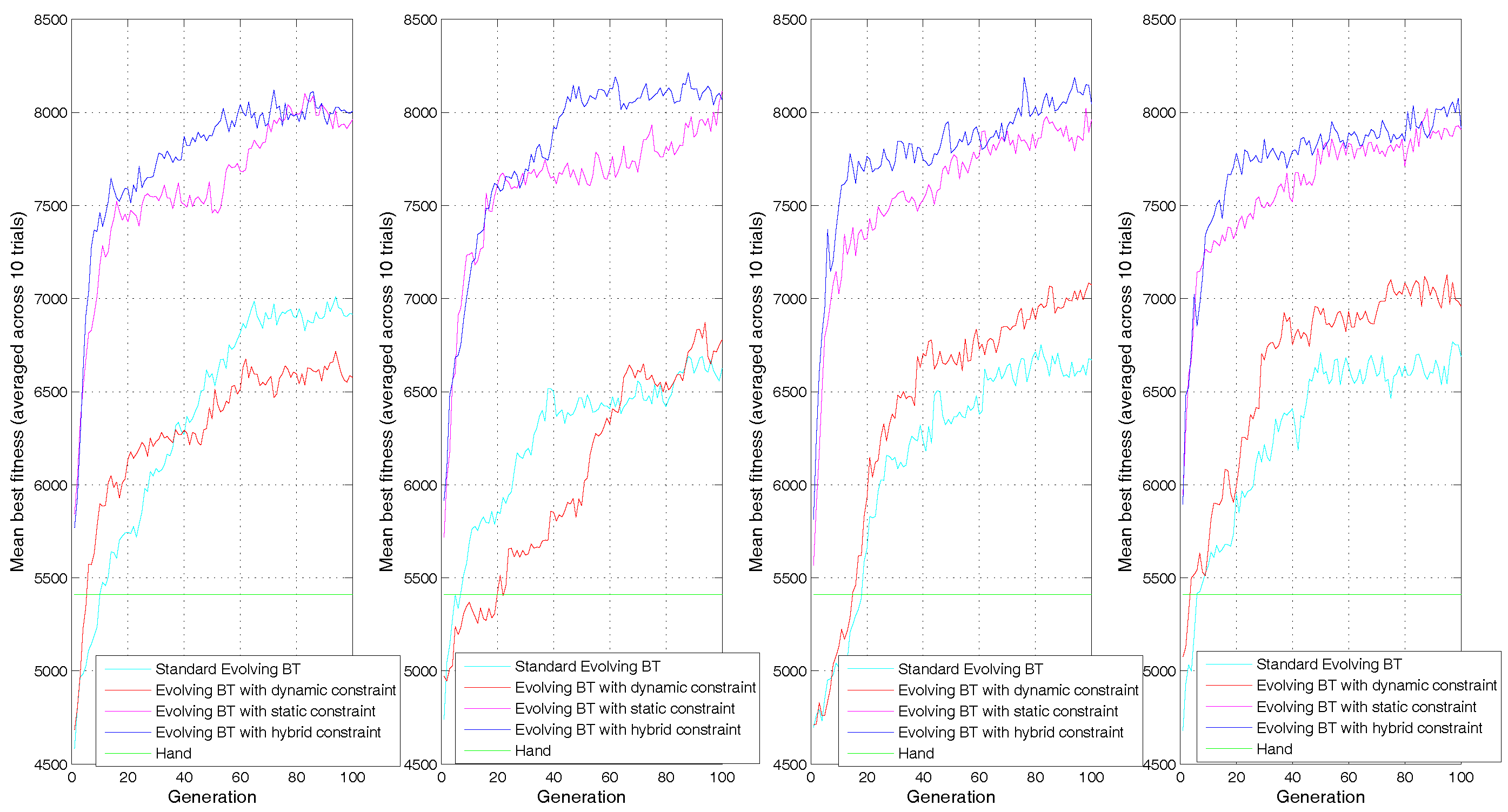
As the dynamic constraint is proposed to accelerate learning directly, we first check the learning speed of different approaches under different parameters. Figure 6 shows the learning curves of mean best fitness with variable crossover probability 0.6, 0.7, 0.8 and 0.9 respectively, Figure 7 shows the learning curves of mean best fitness with variable new chromosomes 0.1, 0.2 and 0.3 respectively, and Figure 8 shows the learning curves of mean best fitness with variable mutation probability 0.01 and 0.1 respectively.
In all the learning curves, the approaches EBT-HC and EBT-SC are obviously faster than the approaches EBT and EBT-DC and get higher best mean fitness in the end of evolution.That is because the static constraint can provide well-designed possible tree structure based on common design pattern, which would reduce search space effectively and find a good solution easier. However, the static structure can only support limited use of control nodes, selector and sequence.
Figure 6 shows the learning curves of four evolving approaches under the values of crossover probability 0.6, 0.7, 0.8 and 0.9 respectively. We can see that, in all 4 subfigures, the approach EBT-HC is faster than the EBT-SC and achieves comparable best mean fitness in the end of evolution. When the crossover probability is 0.6, the fitness of EBT-DC climbs obviously faster than the EBT within the first 20 generations, but becomes slower after that. In the end of evolution, the EBT-DC gets a lower mean best value fitness than EBT. It indicates that the EBT-DC converges prematurely to a local minimal value. When the crossover probability grows to 0.7, the EBT-DC performs slower than EBT in most generations, but converges to a similar final mean best fitness with EBT. When the crossover probabilities are 0.8 and 0.9 respectively, the EBT-DC begins to show better performance on average than EBT at generations of 20 and 10 respectively, and finally achieve a higher mean best fitness at generation 100. The results show that the dynamic constraint is robust to help EBT-SC to accelerate learning, while in partial values 0.8, 0.9 of crossover probability, it can help EBT to accelerate learning.
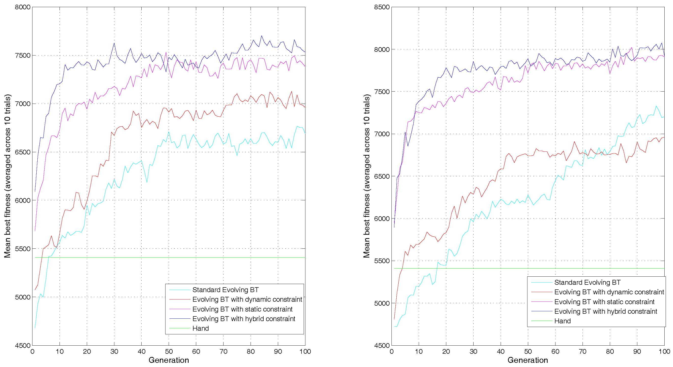
Figure 7 show the learning curves under the values of new chromosome proportion 0.1, 0.2 and 0.3 respectively. We can see that in all 3 subfigures, the EBT-DC is obviously faster than EBT to achieve higher fitness within limited generations. When the new chromosomes is 0.1, the EBT-HC shows similar performance with EBT-SC in term of learning speed and final mean best fitness. As the new chromosomes grow to 0.2 and 0.3, the EBT-HC learns faster at early stage of generation 10 and middle stage of generation 60, and finaly achieve a slight higher final best fitness than EBT-SC. The results show that the dynamic constraint can accelerate learning of EBT and get a better final best fitness, while for EBT-SC, it can help to accelerate learning in new chromosomes 0.2 and 0.3.
In Figure 8 we can see that, when the mutation probability is 0.01, the EBT-DC learns faster than EBT and converges to a higher mean best fitness in the end of evolution. For the EBT-HC, it climbs faster than EBT-SC within generation 10 and gets a comparable mean best fitness. When the mutation probability is 0.1, the EBT-DC is faster than EBT at early stage but converges to a lower value than EBT in the end of evolution. The EBT-HC learns faster than EBT-SC at early stage and both two converge to a similar mean best fitness in the end. It should be noted that, the final mean best fitness of EBT-SC and EBT-HC under mutation probability 0.01 are obviously lower than those under mutation probability of 0.1. In both the approaches EBT-SC and EBT-HC, the adjacent terminal child nodes are regarded as a sequential behavior block and the crossover is carried out only between nodes/blocks with the same type, thus the possible behavior blocks will remain unchanged and the population diversity declines to a great extent. The results indicate that under both mutation probabilities, the dynamic constraint can help EBT and EBT-SC to accelerate learning, but the approaches EBT-SC and EBT-HC need a bigger mutation probability to maintain higher diversity in generated blocks.
On the whole, in most tested GA parameters, the dynamic constraint can help standard evolving BT and evolving approach with static constraint to accelerate learning speed and achieve better individuals with higher final fitness.
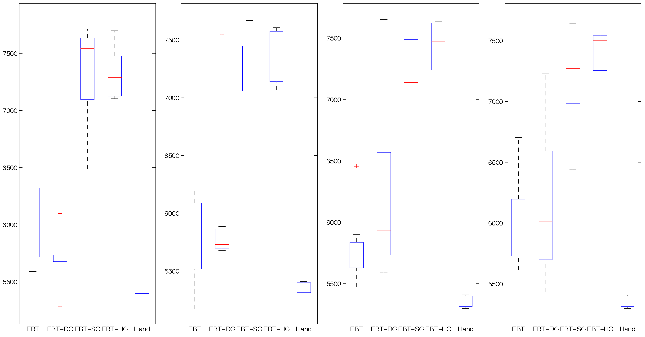
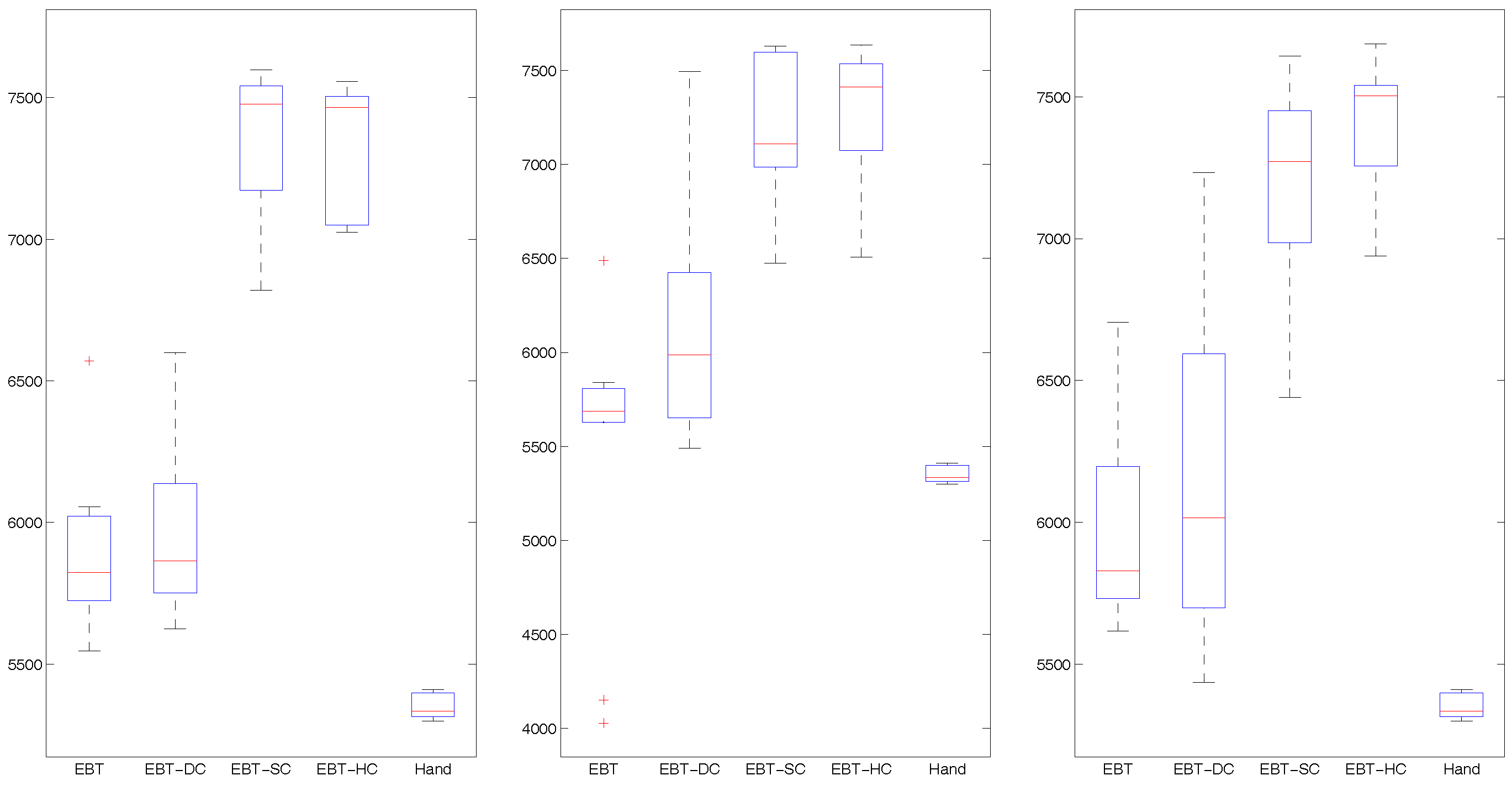
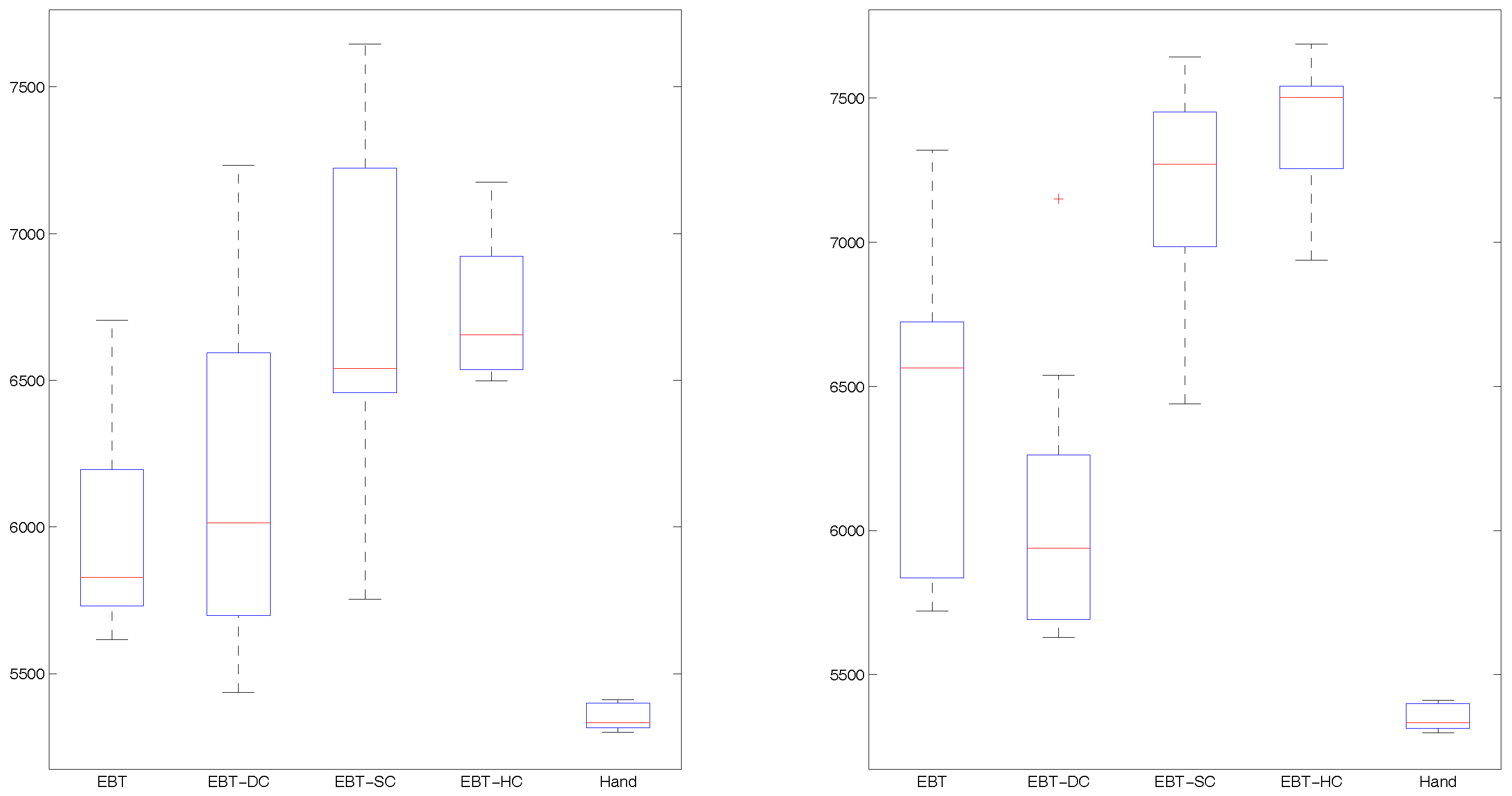
For agent behavior modeling, another important concern is whether we can get an expected behavior model satisfying the evaluation criterions of domain expert. In evolving BTs for behavior modeling specifically, the goal is to produce the best BT individual with higher fitness than other existing approaches in simulation tests. Thus, we will check the average fitness of the best individual generated by different approaches. Table 2 shows all the average fitness results of mean and standard deviation under different GA parameters. Figure 9 shows the results distribution of mean best fitness with variable crossover probability 0.6, 0.7, 0.8 and 0.9 respectively, Figure 10 shows the results distribution of mean best fitness with variable new chromosomes 0.1, 0.2 and 0.3 respectively, and Figure 11 shows the results distribution of mean best fitness with variable mutation probability 0.01 and 0.1 respectively.
From Table 2 we can see that, when crossover probabilities are 0.7, 0.8 and 0.9, the EBT-HC can achieve bigger means of 7371.0, 7419.5 and 7406.5 than the EBT-SC with 7174.5, 7169.6 and 7173.5 respectively, and lower standard deviation of 224.0, 218 and 258.2 than the EBT-SC with 454.0, 353.1 and 402.2 respectively. In the boxplot Figure 9 we also can see that, the whole distribution of all the individuals in EBT-HC is above the distribution in EBT-SC. All three lower adjacent values in EBT-HC are higher than the lower whiskers in EBT-SC, which indicates the lowest individual in EBT-HC is better than more than 25% of individuals in EBT-SC. When the crossover probability is 0.6, the EBT-HC gets slightly smaller values of mean and standard deviation than EBT-SC. In terms of EBT-DC and EBT, we can see when the crossover probability is 0.6, the EBT-DC gets a lower 5734.6 than EBT with 6011.8. When the value grows to 0.7, the EBT-DC achieves similar mean with EBT, and when the value is 0.8 and 0.9, the EBT-DC achieves higher mean than EBT. In most cases, the standard deviation of EBT-DC is bigger than EBT. Those results indicate that the dynamic constraint can help EBT-DC and EBT-HC achieve better final solutions than EBT and EBT-SC respectively under bigger crossover probability like 0.8 and 0.9. The EBT-DC can achieve comparable final solution under crossover probability 0.8 and 0.9, but result in unstable solution. While for EBT-HC, it achieves higher and more stable final solution than EBT-SC.
In Table 2 and Figure 10, when the new chromosomes is 0.1, the EBT-HC and EBT-DC get similar results with EBT-SC and EBT respectively. When the new chromosomess are 0.2 and 0.3, the EBT-HC and EBT-DC get higher mean and median than EBT-SC and EBT respectively. The EBT-DC gets bigger standard deviation than EBT, while EBT-HC gets smaller standard deviation than EBT-SC. That may be because when new chromosome proportion is lower as 0.1, the population diversity is declined, which may increase the risk of dynamic constraint trapped local minimum. Thus, we should use slight bigger new chromosome proportion like 0.2 and 0.3.
In Table 2 and Figure 11, when the mutation probability is 0.01, the EBT-DC gets higher mean and median but larger distribution. Comparing with EBT-SC, EBT-HC gets higher median, similar mean and smaller standard deviation. When the mutation probability is 0.1, EBT-DC gets obviously lower mean and median than EBT, EBT-HC gets higher median and mean than EBT-SC. It should be noted that the values of EBT-SC and EBT-DC under mutation probability 0.01 are obviously lower than those values under mutation probability 0.1. That is because the static constraint on crossover will decline the diversity of swapped behavior blocks, we should set a big mutation probability for the EBT-SC and EBT-HC.
Those results show that the EBT-HC can achieve higher and more stable solution than EBT-SC in most tested parameter values. While for EBT-DC, the dynamic constraint can help it to achieve higher mean but bigger standard deviation when the population diversity is declined.
From above statistical experimental results of learning curves and final best individuals, we can draw conclusions that the EBT-DC with dynamic constraint can get faster learning speed and comparable final solution than EBT. However the results are more unstable. The EBT-HC can learn faster and achieve higher and more stable final solution than EBT-SC. Considering the sensitivity for variable parameters, the EBT-DC is a bit sensitive to the learning parameters, especially the crossover probability, the EBT-HC is more robust than the EBT-DC under tested GA parameters. Both EBT-HC and EBT-DC need a bigger crossover probability, a slight bigger new chromosome and a bit bigger mutation probability to increase the population diversity, which is important for approaches with dynamic constraint, especially EBT-DC.
The static structural constraint can effectively restrict the search space to find better solution faster. At the same time, it is easier to escape from the local optimal under existing genetic operators. When applying the dynamic constraint in the evolving approach with static constraint, it is easier to find valuable and tidy frequent sub-trees to accelerate learning for the hybrid approach, which will accelerate optimal tree structure composition. While in standard evolving BT approach, the search space is very big and many solutions found are inefficient with inactive nodes never executed. When the changes of GA parameters reduce the population diversity, such as a small crossover probability of 0.6, it is harder for the standard evolving BT approach to escape from the local minimum than the approach with static constraint. When applying dynamic constraint in standard evolving approach, the preference for crossover may increase the chance trapped in local minimum, which leads to the result more unstable.
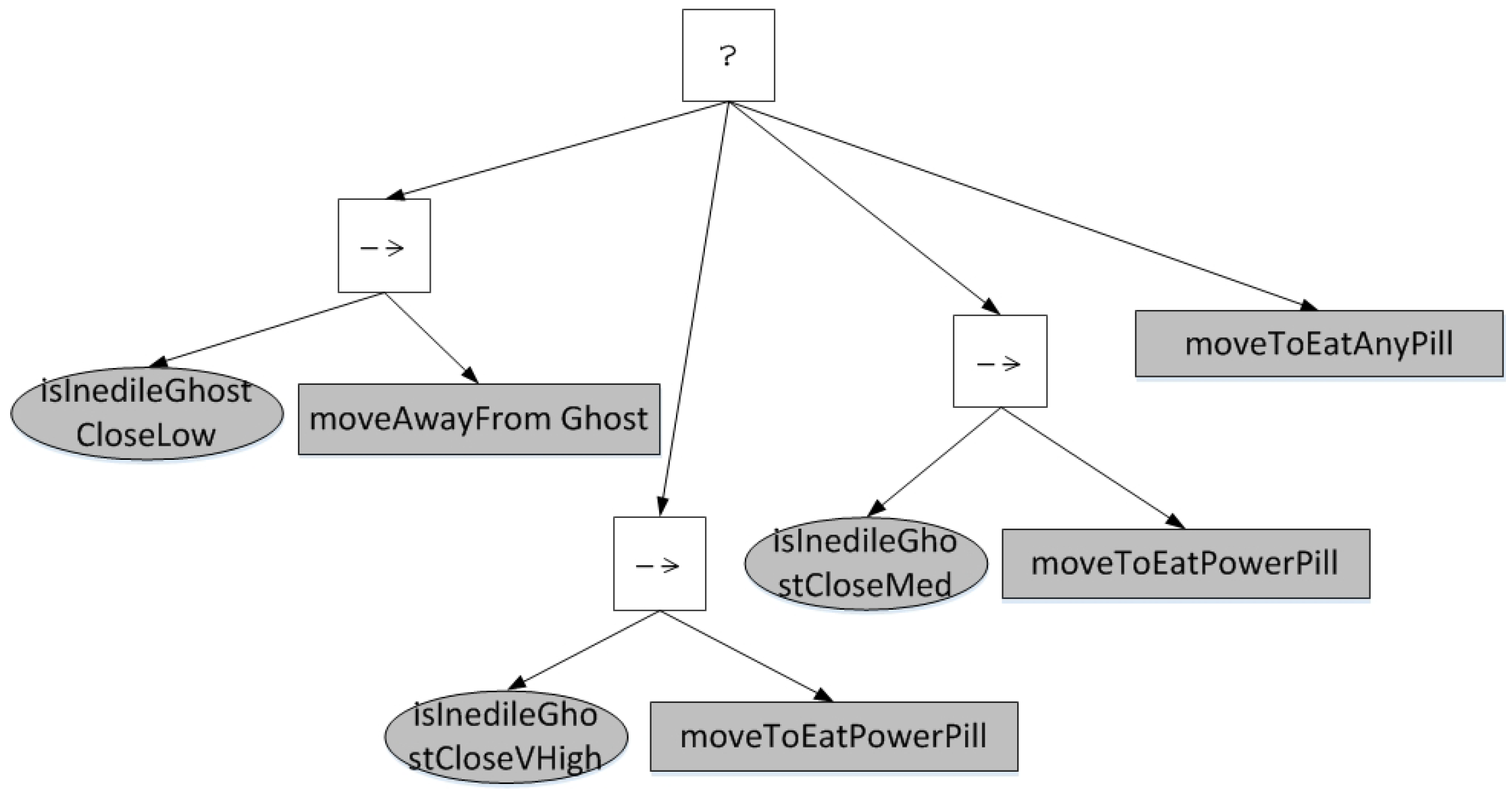
In the experiment, we also record the final generated BTs and the mined frequent sub-trees to check the intuitive products of behavior modeling. Figure 12 shows a BT generated by the approach EBT-HC. We can see that it is easy to understand the logic behind the controller. It divides the decision-making of full state space into some specific situations to deal with. For example, when the distance to the nearest inedible ghost is low, the agent chooses to evade from the ghost. When the distance to the nearest inedible ghost is very high, the agent chooses to move to eat the nearest power pill. When all the above conditions are not meted, the action ‘moveToEatAnyPill’ is executed with the lowest priority to execute. Comparing with the handcrafted BT, it seems to be plausible. An interesting phenomenon is that the generated BT does not check the condition ‘isEdibleGhostClose’ and chooses action ‘moveTowardsGhost’ as the handcrafted BT does, it is out of our expectation but actually reaches a higher fitness than the handcrafted BT. It may be the expected result of large number of game runs considering the randomness. This phenomenon acting in a different way as human can be regarded as computational creativity that are not found by humans [5].
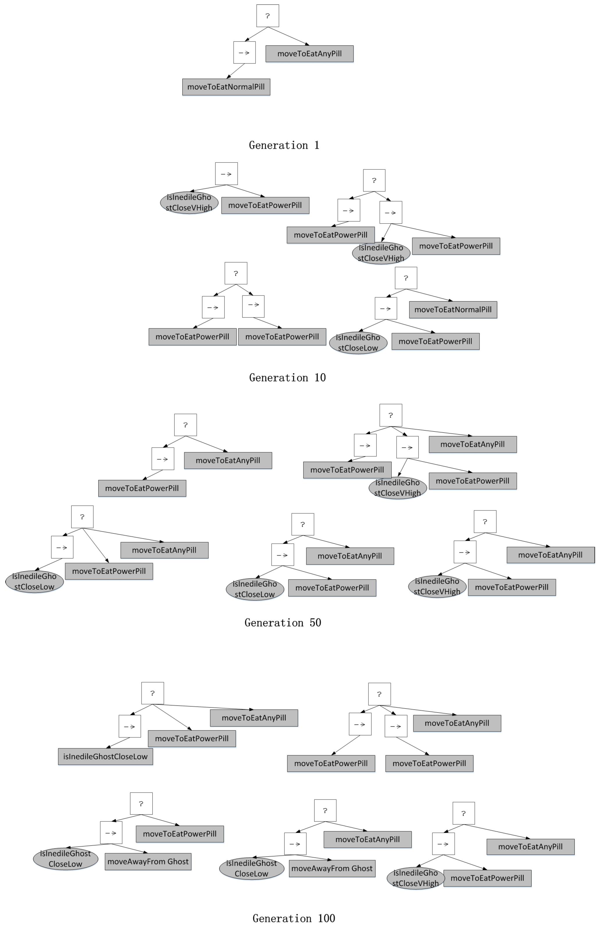
Figure 13 shows the sub-trees evolution of the proposed evolving BT approach with hybrid constraints over generations. Because of the limitation of space, we just show the distinct sub-trees found at generation 1, 10, 50 and 100. We can see that at generation 1, only a simple sub-tree is mined which leads agent to move to a pill, which can be formed in most initial individuals with higher ranked fitness. Please note that if a frequent sub-tree is a child of another frequent sub-tree, we only record the one with bigger size. So in fact the action nodes ‘moveToAnyPill’ and ‘moveToNormalPill’ are both frequent. For the next generation, the higher ranked individuals with the frequent sub-tree will protect the structure with a little preference, which encourage individuals to search better solution around this structure. At generation 10, we can see that the preponderant sub-tree of generation 1 is no longer frequent. More valuable frequent sub-trees are found which represent the reactive decision-making or action priority for some local situations. For example, when the distance to the nearest inedible ghost is very high, the agent will choose to seek to eat power pill which can provide the agent attack capacity. At generation 50, we can see that some bigger sub-trees become frequent based on the frequent sub-tree found at generation 10, some sub-trees are still frequent those in generation 10. At the same time, some more appropriate action priority is found to replace original structure, for example the node ‘moveToAnyPill’ is set as the node with lowest priority, which seems to be reasonable. At generation 100, some sub-trees at generation 10 are still frequent, which indicate that they are really necessary building blocks of optimal solution. While some new frequent sub-trees are found such as ‘moveAwayFromGhost’, some frequent sub-trees in generation 50 are changed. Comparing with the final structure in Figure 12, we can see that most frequent sub-trees mined at generation 100 are the sub-trees of the final best model. The evolution of sub-trees reflects transparently that how the final full model be composed of the frequent sub-tree found generation by generation, which can justify our approach further. Additionally, those sub-trees can be used to facilitate the BT design by domain expert.
5. Conclusions and Future Works
This paper proposed a modified evolving behavior trees approach, named evolving BTs with hybrid constraints (EBT-HC), to facilitate behavior modeling for autonomous agents in simulation and computer games. Our main contribution is a novel idea of dynamic constraint to improve the evolution of Behavior Trees, which discovers the frequent preponderant sub-trees and adjusts nodes crossover probability to accelerate preponderant structure combination. To improve the evolving BT with only dynamic constraint further, we proposed the evolving BTs approach with hybrid constraints by combing the existing static structural constraint with our dynamic constraint. The hybrid EBT-HC can further accelerate behavior learning and find better solutions without the loss of the domain-independence. Preliminary experiments on ’Ms Pac-Man vs Ghosts’ benchmark showed that the proposed EBT-HC approach can produce plausible behaviors than other approaches. The stable final best individual with higher fitness satisfies the goal of generating better behavior policy based on evaluation criteria provided by domain expert. The fast and stable learning curve showed the advantage of hybrid constraints to speed up convergence. From the perspective of tree design and implementation, the generated BTs are human readable and easy to analyze and fine-tune, which can be a promising initial step for transparent behavior modeling automatically.
There are some avenues of research to improve this study. Firstly, the proposed approach should be validated in more complex task scenarios and configurations for behavior modeling automatically. In current work, the Pac-Man game is configured as a simple and typical simulation environment to validate proposed approach. However, the interaction between the learning technique and the agent environment is nontrivial. The environmental model, behavior evaluation function, perception, and action sets are critical for behavior performance. Thus, more complex scenarios, such as bigger state-space representation, partial observation or multiple agents in real-time strategy game [31], should be considered to provide rich agent learning environment to validate the proposed approach. On the other hand, it is important to research automatic learning for appropriate parameters setting in GP systems. It is necessary to broaden the applications of proposed approach in more scenarios and configurations.
Another interesting research topic is learning behavior trees from observation. For behavior modeling through experiential learning, it is measured by how well the task is performed based on the evaluation criteria provided by experts. However, the optimal behavior may be inappropriate or unnatural. Thus, there are a few works of learning BTs from observation emerged but still an open problem [7,25]. We believe GP is a promising method and the frequent sub-tree mining can be a potential tool to facilitate behavior block building and accelerate learning. The possible issue behind the method is the similarity metric to evaluate the generated behavior. In [32], the authors investigate a gamalyzer-based play trace metric to measure the difference between two play traces in computer games. Based on above techniques, we can develop a model-free framework to generate BT by learning from training examples.
Author Contributions
Q.Z. and J.Y. conceived and designed the paper structure and the experiments; Q.Z. performed the experiments; Q.Y. and Y.Z. contributed with materials and analysis tools.
Funding
This work was partially supported by the National Science Foundation (NSF) project 61473300, CHINA.
Acknowledgments
This work was partially supported by the National Science Foundation (NSF) project 61473300, CHINA. The authors would like to thank the helpful discussions and suggestions with Xiangyu Wei, Kai Xu and Weilong Yang.
Conflicts of Interest
The authors declare no conflict of interest. The founding sponsors had no role in the design of the study; in the collection, analysis, or interpretation of data; in the writing of the manuscript, and in the decision to publish the results.
Abbreviations
The following abbreviations are used in this manuscript:
| BTs | Behavior Trees |
| FSMs | Finite State Machines |
| NPC | Non-player Characters |
| CGF | Computer-Generated Force |
| GP | Genetic Programming |
| RL | Reinforcement Learning |
| LfO | Learning from Observation |
| NN | Neural Network |
| NSF | National Science Foundation |
References
- Tirnauca, C.; Montana, J.L.; Ontanon, S.; Gonzalez, A.J.; Pardo, L.M. Behavioral Modeling Based on Probabilistic Finite Automata: An Empirical Study. Sensors 2016, 16, 958. [Google Scholar] [CrossRef] [PubMed]
- Toubman, A.; Poppinga, G.; Roessingh, J.J.; Hou, M.; Luotsinen, L.; Lovlid, R.A.; Meyer, C.; Rijken, R.; Turcanik, M. Modeling CGF Behavior with Machine Learning Techniques: Requirements and Future Directions. In Proceedings of the 2015 Interservice/Industry Training, Simulation, and Education Conference, Orlando, FL, USA, 30 November–4 December 2015; pp. 2637–2647. [Google Scholar]
- Diller, D.E.; Ferguson, W.; Leung, A.M.; Benyo, B.; Foley, D. Behavior modeling in commercial games. In Proceedings of the 2004 Conference on Behavior Representation in Modeling and Simulation (BRIMS), Arlington, VA, USA, 17–20 May 2004; pp. 17–20. [Google Scholar]
- Kamrani, F.; Luotsinen, L.J.; Løvlid, R.A. Learning objective agent behavior using a data-driven modeling approach. In Proceedings of the IEEE International Conference on Systems, Man, and Cybernetics, Budapest, Hungary, 9–12 October 2017; pp. 002175–002181. [Google Scholar]
- Luotsinen, L.J.; Kamrani, F.; Hammar, P.; Jändel, M.; Løvlid, R.A. Evolved creative intelligence for computer generated forces. In Proceedings of the IEEE International Conference on Systems, Man, and Cybernetics, Budapest, Hungary, 9–12 October 2017; pp. 003063–003070. [Google Scholar]
- Yao, J.; Huang, Q.; Wang, W. Adaptive human behavior modeling for air combat simulation. In Proceedings of the 2015 IEEE/ACM 19th International Symposium on Distributed Simulation and Real Time Applications (DS-RT), Chengdu, China, 14–16 October 2015; pp. 100–103. [Google Scholar]
- Sagredo-Olivenza, I.; Gómez-Martín, P.P.; Gómez-Martín, M.A.; González-Calero, P.A. Trained Behavior Trees: Programming by Demonstration to Support AI Game Designers. IEEE Trans. Games 2017. [Google Scholar] [CrossRef]
- Sekhavat, Y.A. Behaivor Trees for Computer Games. Int. J. Artif. Intell. Tools 2017, 1, 1–27. [Google Scholar]
- Rabin, S. AI Game Programming Wisdom 4; Nelson Education: Scarborough, ON, Canada, 2014; Volume 4. [Google Scholar]
- Colledanchise, M.; Ögren, P. Behavior Trees in Robotics and AI: An Introduction. arXiv, 2017; arXiv:1709.00084. [Google Scholar]
- Nicolau, M.; Perezliebana, D.; Oneill, M.; Brabazon, A. Evolutionary Behavior Tree Approaches for Navigating Platform Games. IEEE Trans. Comput. Intell. AI Games 2017, 9, 227–238. [Google Scholar] [CrossRef] [Green Version]
- Perez, D.; Nicolau, M.; O’Neill, M.; Brabazon, A. Evolving behaviour trees for the mario AI competition using grammatical evolution. In Proceedings of the European Conference on the Applications of Evolutionary Computation, Torino, Italy, 27–29 April 2011; pp. 123–132. [Google Scholar]
- Lim, C.U.; Baumgarten, R.; Colton, S. Evolving behaviour trees for the commercial game DEFCON. In Proceedings of the European Conference on the Applications of Evolutionary Computation, Torino, Italy, 7–9 April 2010; pp. 100–110. [Google Scholar]
- Mcclarron, P.; Ollington, R.; Lewis, I. Effect of Constraints on Evolving Behavior Trees for Game AI. In Proceedings of the International Conference on Computer Games Multimedia & Allied Technologies, Los Angeles, CA, USA, 15–18 November 2016. [Google Scholar]
- Press, J.R.K.M. Genetic programming II: Automatic discovery of reusable programs. Comput. Math. Appl. 1995, 29, 115. [Google Scholar]
- Poli, R.; Langdon, W.B.; Mcphee, N.F. A Field Guide to Genetic Programming; lulu.com: Morrisville, NC, USA, 2008; pp. 229–230. [Google Scholar]
- Scheper, K.Y.W.; Tijmons, S.; Croon, G.C.H.E.D. Behavior Trees for Evolutionary Robotics. Artif. Life 2016, 22, 23–48. [Google Scholar] [CrossRef] [PubMed]
- Champandard, A.J. Behaivor Trees for Next-gen Game AI. Available online: http://aigamedev.com/insider/presentations/behavior-trees/ (accessed on 12 December 2007).
- Zhang, Q.; Yin, Q.; Xu, K. Towards an Integrated Learning Framework for Behavior Modeling of Adaptive CGFs. In Proceedings of the IEEE 9th International Symposium on Computational Intelligence and Design (ISCID), Hangzhou, China, 10–11 December 2016; Volume 2, pp. 7–12. [Google Scholar]
- Fernlund, H.K.G.; Gonzalez, A.J.; Georgiopoulos, M.; Demara, R.F. Learning tactical human behavior through observation of human performance. IEEE Trans. Syst. Man Cybern. Part B Cybern. 2006, 36, 128. [Google Scholar] [CrossRef]
- Stein, G.; Gonzalez, A.J. Building High-Performing Human-Like Tactical Agents Through Observation and Experience; IEEE Press: Piscataway, NJ, USA, 2011; p. 792. [Google Scholar]
- Teng, T.H.; Tan, A.H.; Tan, Y.S.; Yeo, A. Self-organizing neural networks for learning air combat maneuvers. In Proceedings of the IEEE International Joint Conference on Neural Networks (IJCNN), Brisbane, Australia, 10–15 June 2012; pp. 1–8. [Google Scholar]
- Ontañón, S.; Mishra, K.; Sugandh, N.; Ram, A. Case-Based Planning and Execution for Real-Time Strategy Games. In Proceedings of the International Conference on Case-Based Reasoning: Case-Based Reasoning Research and Development, Northern Ireland, UK, 13–16 August 2007; pp. 164–178. [Google Scholar]
- Aihe, D.O.; Gonzalez, A.J. Correcting flawed expert knowledge through reinforcement learning. Expert Syst. Appl. 2015, 42, 6457–6471. [Google Scholar] [CrossRef]
- Robertson, G.; Watson, I. Building behavior trees from observations in real-time strategy games. In Proceedings of the International Symposium on Innovations in Intelligent Systems and Applications, Madrid, Spain, 2–4 September 2015; pp. 1–7. [Google Scholar]
- Dey, R.; Child, C. Ql-bt: Enhancing behaviour tree design and implementation with q-learning. In Proceedings of the IEEE Conference on Computational Intelligence in Games (CIG), Niagara Falls, ON, Canada, 11–13 August 2013; pp. 1–8. [Google Scholar]
- Zhang, Q.; Sun, L.; Jiao, P.; Yin, Q. Combining Behavior Trees with MAXQ Learning to Facilitate CGFs Behavior Modeling. In Proceedings of the 4th International Conference on IEEE Systems and Informatics (ICSAI), Hangzhou, China, 11–13 November 2017. [Google Scholar]
- Asai, T.; Abe, K.; Kawasoe, S.; Arimura, H.; Sakamoto, H.; Arikawa, S. Efficient Substructure Discovery from Large Semi-structured Data. In Proceedings of the Siam International Conference on Data Mining, Arlington, Arlington, VA, USA, 11–13 April 2002. [Google Scholar]
- Chi, Y.; Muntz, R.R.; Nijssen, S.; Kok, J.N. Frequent Subtree Mining—An Overview. Fundam. Inf. 2005, 66, 161–198. [Google Scholar]
- Williams, P.R.; Perezliebana, D.; Lucas, S.M. Ms. Pac-Man Versus Ghost Team CIG 2016 Competition. In Proceedings of the IEEE Conference on Computational Intelligence and Games (CIG), Santorini, Greece, 20–23 September 2016. [Google Scholar]
- Christensen, H.J.; Hoff, J.W. Evolving Behaviour Trees: Automatic Generation of AI Opponents for Real-Time Strategy Games. Master’s Thesis, Norwegian University of Science and Technology, Trondheim, Norway, 2016. [Google Scholar]
- Osborn, J.C.; Samuel, B.; Mccoy, J.A.; Mateas, M. Evaluating play trace (Dis)similarity metrics. In Proceedings of the AIIDE, Raleigh, NC, USA, 3–7 October 2014. [Google Scholar]
Figure 1.
The graphical representation of a behavior tree nodes used.

Figure 2.
The proposed evolving behavior tree framework, behavior tree (BT).

Figure 3.
The proposed crossover operation with frequent sub-trees.

Figure 4.
An example behavior tree designed using static structural constraint.

Figure 5.
The benchmark ‘Ms. Pac-Man vs. Ghosts’ used in the experiments.

Figure 6.
Learning curves of different approaches with variable crossover probability 0.6, 0.7, 0.8 and 0.9.
Figure 6.
Learning curves of different approaches with variable crossover probability 0.6, 0.7, 0.8 and 0.9.

Figure 7.
Learning curves of different approaches with variable new chromosomes 0.1, 0.2 and 0.3.

Figure 8.
Learning curves of different approaches with variable mutation probability 0.01 and 0.1.

Figure 9.
Boxplot results for the best generated BTs with variable crossover probability 0.6, 0.7, 0.8 and 0.9.
Figure 9.
Boxplot results for the best generated BTs with variable crossover probability 0.6, 0.7, 0.8 and 0.9.

Figure 10.
Boxplot results for the best generated BTs with variable new chromosomes 0.1, 0.2 and 0.3.
Figure 10.
Boxplot results for the best generated BTs with variable new chromosomes 0.1, 0.2 and 0.3.

Figure 11.
Boxplot results for the best generated BTs with variable mutation probability 0.01 and 0.1.
Figure 11.
Boxplot results for the best generated BTs with variable mutation probability 0.01 and 0.1.

Figure 12.
A BT generated by the proposed EBT-HC approach.

Figure 13.
An evolution of frequent sub-trees found over generation by EBT-HC.


Table 1.
Parameter settings for different tested approaches, evolving BTs with only dynamic constraint (EBT-DC), evolving BTs with hybrid constraints (EBT-HC).
Table 1.
Parameter settings for different tested approaches, evolving BTs with only dynamic constraint (EBT-DC), evolving BTs with hybrid constraints (EBT-HC).
| Approach | Parameter | Value |
|---|---|---|
| fixed to all approaches | population size | 100 |
| generations | 100 | |
| initial min depth | 2 | |
| initial max depth | 3 | |
| selection tournament size | ||
| parsimony coefficient | 0.7 | |
| variable to all approaches | new chromosomes | |
| crossover probability | 0.6/0.7/0.8/0.9 | |
| reproduction probability | 0.4/0.3/0.2/0.1 | |
| mutation probability | 0.01/0.1 | |
| EBT-DC/EBT-HC | superior individuals | |
| the minimal support | 0.3 | |
| the minimal node size | 3 | |
| the maximal node size | 15 | |
| the minimal terminal node size | 2 | |
| the discount factor | 0.9 |
Table 2.
Mean and standard deviation of the best individual of four evolving approaches under different parameters settings. The mean and standard deviation of the baseline handcrafted BT are 5351.3 and 47.6 (with 95% confidence interval), evolving BTs approach (EBT), existing ‘static’ structural constraint (EBT-SC).
| EBT | EBT-DC | EBT-SC | EBT-HC | ||
|---|---|---|---|---|---|
| Crossover probability | 0.6 | 6011.8 ± 320.2 | 5734.6 ± 347.3 | 7344.8 ± 428.4 | 7324.5 ± 221.8 |
| 0.7 | 5768.0 ± 341.6 | 5930.9 ± 572.2 | 7174.5 ± 454.0 | 7371.0 ± 224.0 | |
| 0.8 | 5781.7 ± 267.9 | 6274.8 ± 728.5 | 7169.6 ± 353.1 | 7419.5 ± 218.5 | |
| 0.9 | 5978.8 ± 361.1 | 6168.4 ± 609.4 | 7173.5 ± 402.2 | 7406.5 ± 258.2 | |
| new chromosomes | 0.1 | 5886.4 ± 282.9 | 5962.3 ± 311.3 | 7353.6 ± 274.9 | 7350.0 ± 221.4 |
| 0.2 | 5471.7 ± 769.9 | 6105.8 ± 592.1 | 7197.0 ± 369.3 | 7300.5 ± 344.9 | |
| 0.3 | 5978.8 ± 361.1 | 6168.4 ± 609.4 | 7173.5 ± 402.2 | 7406.5 ± 258.2 | |
| Mutation probability | 0.01 | 5978.8 ± 361.1 | 6168.4 ± 609.4 | 6720.7 ± 606.6 | 6737.2 ± 262.6 |
| 0.1 | 6456.9 ± 523.0 | 6087.7 ± 473.0 | 7173.5 ± 402.2 | 7406.5 ± 258.2 |
© 2018 by the authors. Licensee MDPI, Basel, Switzerland. This article is an open access article distributed under the terms and conditions of the Creative Commons Attribution (CC BY) license (http://creativecommons.org/licenses/by/4.0/).
Share and Cite
MDPI and ACS Style
Zhang, Q.; Yao, J.; Yin, Q.; Zha, Y. Learning Behavior Trees for Autonomous Agents with Hybrid Constraints Evolution. Appl. Sci. 2018, 8, 1077. https://doi.org/10.3390/app8071077
AMA Style
Zhang Q, Yao J, Yin Q, Zha Y. Learning Behavior Trees for Autonomous Agents with Hybrid Constraints Evolution. Applied Sciences. 2018; 8(7):1077. https://doi.org/10.3390/app8071077
Chicago/Turabian StyleZhang, Qi, Jian Yao, Quanjun Yin, and Yabing Zha. 2018. "Learning Behavior Trees for Autonomous Agents with Hybrid Constraints Evolution" Applied Sciences 8, no. 7: 1077. https://doi.org/10.3390/app8071077
Note that from the first issue of 2016, this journal uses article numbers instead of page numbers. See further details here.